One-Step Stochastic Processes Simulation Software Package

Abstract

Background

It is assumed that the introduction of stochastic in mathematical model makes it more adequate. But there is virtually no methods of coordinated (depended on structure of the system) stochastic introduction into deterministic models. Authors have improved the method of stochastic models construction for the class of one-step processes and illustrated by models of population dynamics. Population dynamics was chosen for study because its deterministic models were sufficiently well explored that allows to compare the results with already known ones.

Purpose

To optimize the models creation as much as possible some routine operations should be automated. In this case, the process of drawing up the model equations can be algorithmized and implemented in the computer algebra system. Furthermore, on the basis of these results a set of programs for numerical experiment can be obtained .

Method

The computer algebra system Axiom is used for analytical calculations implementation. To perform the numerical experiment FORTRAN and Julia languages are used. The method Runge–Kutta method for stochastic differential equations is used as numerical method.

Results

The program compex for creating stochastic one-step processes models is constructed. Its application is illustrated by the predator-prey population dynamic system.

Conclusions

Computer algebra systems are very convenient for the purposes of rapid prototyping in mathematical models design and analysis.

I Introduction

This work corresponds our research on mathematical models stochastization. This item is interesting due to the following problems: the construction of population models from first principles and the introduction of the stochastic into such models (the population dynamics is studied because of similar models introduction in other areas).

The problem of stochastic term introduction arises during mathematical models stochastization. There are several ways to solve this problem. The easiest option is an in the deterministic equation. But when additive stochastic term is introduced some free parameters that require further definition appears. Furthermore, these stochastic terms usually interpreted as an external (rather than structural) random impact. In this regard, we used and improved the stochastic one–step processes models construction method, based on master equation Demidova and Kulyabov (2012); Demidova et al. (2010). Stochastic differential equation is considered as its approximate form. It allows to get the model equations from general principles. Furthermore, deterministic and stochastic parts are derived from the one equation so we can regard it as stochastic and deterministic parts consistency. .

The aim of this work is the software complex development for rapid prototyping construction of stochastic one–step processes models. This complex consists of two blocks. The first block generates the equations of dynamic stochastic process model on the principles similar to chemical kinetic relations describing the investigated process . This block is implemented by means of the computer algebra system - system FriCAS, which is offshoot of Axiom.

The second block is used for the numerical analysis of the resulting model. For numerical solution of deterministic and stochastic models equations some Runge–Kutta different orders methods Debrabant and Röbler (2008); Tocino and Ardanuy (2002) are used.

To illustrate the developed system the well-known population model predator–prey is used Volterra (1976); Bazykin (1998); Bratus et al. (2010).

The structure of the paper is as follows. The basic notation and conventions are introduced in Section II Section III is devoted to brief introduction to the one–step processes stochastization method. Further, in the Section IV the model under investigation is described. In the subsection IV.1 there is a brief reference to standard (deterministic) approach, and in the subsection IV.2 the stochastic extension of our model with the help of the one–step processes stochastization method is obtained.

In the Section V.1 we justify selection of the system, which implements the model equations generating unit. The actual interface of this part of the program complex is described in the Section V.2 .

The possibility of applying Runge–Kutta methods for the analysis of stochastic differential equations is considered in the Section VI. The software interface of the model equations numerical analysis unit is also described in this section. Calculations example is based on the predator–prey model.

II Notations and conventions

1. We use abstract indices notation Penrose and Rindler (1984). In this notation tensor as a whole object is denoted just as an index (e.g., $x^{i}$), components are denoted by underlined index (e.g., $x^{\underline{\vphantom{j}{i}}}$).

2. We will adhere to the following agreements. Latin indices of the middle of the alphabet ($i$, $j$, $k$) will apply to the space of the system state vectors. Latin indices from the beginning of the alphabet ($a$) will relate to the Wiener process space. Latin indices from the end of the alphabet ($p$, $q$) will refer to the indices of the Runge–Kutta method. Greek indices ($\alpha$) will set a number of different interactions in kinetic equations.

3. A Dot over a symbol denotes differentiation with respect to time.

4. The comma in the index denotes partial derivative with respect to corresponding coordinate.

III One-step processes modeling

Let’s briefly review the method of one-step processes stochastization on the basis of Demidova et al. (2014).

We understand one-step processes as Markov processes with continuous time with values in the domain of integers, which transition matrix allows only transitions between neighbouring portions. Also, these processes are known as birth-and-death processes.

One-step processes are subject to the following conditions:

1. If at the moment $t$ the system is in state $i\in\mathbb{Z}_{\geqslant 0}$,then the probability of transition to state $i+1$ in time interval $[t,t+\Delta t]$ is equal to $k^{+}\Delta t+o(\Delta t)$.

2. If at time moment $t$ the system is in state $i\in\mathbb{Z}_{+}$,then the probability of transition to state $i-1$ in the time interval $[t,t+\Delta t]$ is equal to $k^{-}\Delta t+o(\Delta t)$.

3. The probability of transition to a state other than the neighbouring is equal to $o(\Delta t)$.

4. The probability to remain in the same state is equal to $1-(k^{+}+k^{-})\Delta t+o(\Delta t)$.

5. State $i=0$ is an absorbing boundary.

The idea of the one-step processes stochastization method is as follows. Based on the patterns of interaction we construct a master kinetic equation, expand it into a series, leaving only the terms up to and including the second derivative. The resulting equation is the Fokker–Planck equation. In order to get more convenient model we record corresponding Langevin equation. In fact, as we shall see , from the patterns of interaction we will immediately obtain the coefficients of the Fokker–Planck equation (and accordingly, the Langevin equation), so for practical use of the method there is no need to construct the master kinetic equation.

III.1 Interaction schemes

We will describe the state of the system by a state vector $x^{i}\ in\mathbb{R}^{n}$, where $n$ is the system dimension (the state vector is considered as the set of mathematical values, fully describing system). The operator $n^{i}_{j}\in\mathbb{Z}^{n}_{{}\geqslant 0}\times\ setZ^{n}_{{}\geqslant 0}$ defines the state of the system before the interaction and the operator $m^{i}_{j}\in\mathbb{Z}^{n}_{{}\geqslant 0}\times\mathbb{Z}^{n}_{{}\geqslant 0}$ — after.the interaction The result of interaction is a system transition to another state   Demidova et al. (2013); Demidova and Kulyabov (2012).

There are $s$ kinds of different interactions that may happen in the system, $s\in\mathbb{Z}_{+}$. So, instead of $n^{i}_{j}$ and $m^{i}_{j}$ let’s consider the operators $n^{i\alpha}_{j}\in\mathbb{Z}^{n}_{{}\geqslant 0}\times\mathbb{Z}^{n}_{{}\geqslant 0}\times\mathbb{Z}^{s}_{{}\geqslant 0}$ and $m^{i\alpha}_{j}\in\mathbb{Z}^{n}_{{}\geqslant 0}\times\mathbb{Z}^{n}_{{}\geqslant 0}\times\mathbb{Z}^{s}_{{}\geqslant 0}$.

System elements interaction will be described with the interaction schemes similar to chemical kinetic schemes  Gardiner (1985):

$$n^{i\alpha}_{j}x^{j}\overset{k_{\alpha}^{+}}{\underset{k_{\alpha}^{-}}{\rightleftharpoons}}m^{i\alpha}_{j}x^{j},$$ (1)

Here Greek indexes specify the number of interactions and Latin ones specify dimensionality of the system. The state change is given by the operator

$$r_{j}^{i\alpha}=m_{j}^{i\alpha}-n_{j}^{i\alpha}.$$ (2)

Thus, one step interaction $\underline{\vphantom{j}{\alpha}}$ in forward and opposite directions can be written as

$$\begin{gathered}x^{i}\rightarrow x^{i}+r^{i\underline{\vphantom{j}{\alpha}}}_{j}x^{j},\\ x^{i}\rightarrow x^{i}-r^{i\underline{\vphantom{j}{\alpha}}}_{j}x^{j}.\end{gathered}$$ (3)

We can write (1) not in the form of vector equations, but in the more traditional form sums:

$$n^{i\alpha}_{j}x^{j}\delta_{i}\overset{k_{\alpha}^{+}}{\underset{k_{\alpha}^{-}}{\rightleftharpoons}}m^{i\alpha}_{j}x^{j}\delta_{i},$$ (4)

where $\delta_{\underline{\vphantom{j}{i}}}=(1,\ldots,1)$.

Also, we will use the following notation:

$$n^{i\alpha}:=n^{i\alpha}_{j}\delta^{j},\quad m^{i\alpha}:=m^{i\alpha}_{j}\delta^{j},\quad r^{i\alpha}:=r^{i\alpha}_{j}\delta^{j}.$$ (5)

III.2 Master equation

Transition probabilities per unit of time from the state $x^{i}$ to the state $x^{i}+r^{i\underline{\vphantom{j}{\alpha}}}_{j}x^{j}$ (to the state $x^{i}-r^{i\underline{\vphantom{j}{\alpha}}}_{j}x^{j}$) are proportional to the number of $x^{i}$ combination from a set of $n^{i\alpha}$ elements (of $x^{i}$ — combinations from a set of $m^{i\alpha}$) and are given by:

$$\begin{gathered}s^{+}_{\alpha}=k^{+}_{\alpha}\prod_{\underline{\vphantom{j}{i}}=1}^{n}\frac{x^{\underline{\vphantom{j}{i}}}!}{(x^{\underline{\vphantom{j}{i}}}-n^{\underline{\vphantom{j}{i}}\alpha})!},\\ s^{-}_{\alpha}=k^{-}_{\alpha}\prod_{\underline{\vphantom{j}{i}}=1}^{n}\frac{x^{\underline{\vphantom{j}{i}}}!}{(x^{\underline{\vphantom{j}{i}}}-m^{\underline{\vphantom{j}{i}}\alpha})!}.\end{gathered}$$ (6)

Thus, the general form of the master kinetic equation for the states vector $x^{i}$ (it changes by $r^{i\underline{\vphantom{j}{\alpha}}}_{j}x^{j}$ per step), takes the form:

$$\frac{\partial p(x^{i},t)}{\partial t}={}\\ {}=\sum_{\underline{\vphantom{j}{\alpha}}=1}^{m}\left\{\left[s_{\underline{\vphantom{j}{\alpha}}}^{-}(x^{i}+r^{i\underline{\vphantom{j}{\alpha}}},t)p(x^{i}+r^{i\underline{\vphantom{j}{\alpha}}},t)-s_{\underline{\vphantom{j}{\alpha}}}^{+}(x^{i})p(x^{i},t)\right]+\right.\\ \left.+\left[s_{\underline{\vphantom{j}{\alpha}}}^{+}(x^{i}-r^{i\underline{\vphantom{j}{\alpha}}},t)p(x^{i}-r^{i\underline{\vphantom{j}{\alpha}}},t)-s_{\underline{\vphantom{j}{\alpha}}}^{-}(x^{i})p(x^{i},t)\right]\right\}.$$ (7)

III.3 Fokker–Planck equation

UWith the help of the Kramers–Moyal expansion, the Fokker–Planck equation Gardiner (1985) is obtained. For this purpose we will make several assumptions:

1. there are only small jumps, ie $s_{\alpha}(x^{i})$ is a slowly varying function with the change of $x^{i}$;

2. $p(x^{i},t)$ also slowly changes with the change of $x^{i}$.

Then in Fokker–Planck equation (7) one can shift from the point $(x^{i}\pm r^{i\underline{\vphantom{j}{\alpha}}}_{j}x^{j})$ to the point $x^{i}$, and by expanding the right–hand side in a Taylor series and dropping terms of order higher than the second, we obtain Fokker–Planck equation:

$$\frac{\partial p}{\partial t}=-\partial_{i}\left[A^{i}p\right]+\frac{1}{2}\partial_{i}\partial_{j}\left[B^{ij}p\right],$$ (8)

where

$$\begin{gathered}A^{i}:=A^{i}(x^{k},t)=r^{i\underline{\vphantom{j}{\alpha}}}\left[s^{+}_{\underline{\vphantom{j}{\alpha}}}-s^{-}_{\underline{\vphantom{j}{\alpha}}}\right],\\ B^{ij}:=B^{ij}(x^{k},t)=r^{i\underline{\vphantom{j}{\alpha}}}r^{j\underline{\vphantom{j}{\alpha}}}\left[s^{+}_{\underline{\vphantom{j}{\alpha}}}-s^{-}_{\underline{\vphantom{j}{\alpha}}}\right],\qquad\underline{\vphantom{j}{\alpha}}=\overline{1,m}.\end{gathered}$$ (9)

As seen from (9), the coefficients of the Fokker–Planck equation can be obtained directly from (2) and (6), i.e. in practical calculations, there is no need to write the master equation.

III.4 Langevin equation

The Langevin equation corresponds to the Fokker–Planck equation:

$$\mathrm{d}x^{i}=a^{i}\mathrm{d}t+b^{i}_{a}\mathrm{d}W^{a},$$ (10)

where $a^{i}:=a^{i}(x^{k},t)$, $b^{i}_{a}:=b^{i}_{a}(x^{k},t)$, $x^{i}\in\mathbb{R}^{n}$ — is the system state vector, $W^{a}\in\mathbb{R}^{m}$ — $m$-dimensional Wiener process. Wiener process is implemented as $\mathrm{d}W=\varepsilon\sqrt{\mathrm{d}t}$, where $\varepsilon\sim N(0,1)$ is normal distribution with average $0$ and variance $1$. Latin indexes from the middle of the alphabet denote the values related to the state vectors (dimension of the space is $n$), and Latin indexes from the beginning of the alphabet denote the values related to the Wiener process vector (dimension of the space is $m\leqslant n$).

The connection between the equation (8) and (10) expressed by the following relationships:

$$A^{i}=a^{i},\qquad B^{ij}=b^{i}_{a}b^{ja}.$$ (11)

We will use Ito interpretation. Under the Ito interpretation, differential of complex functions does not obey the standard formulas of analysis. To calculate it rule or Ito lemma are used.

Let $f:=f(x^{k},t)$ is a function of a random process $x^{k}(t)$, $f\in\mathrm{C}^{2}$. Then the formula of the differential is Øksendal (2003):

$$\mathrm{d}f=\left[\partial_{t}f+a^{i}f_{,i}+\frac{1}{2}b^{i}_{a}b^{ia}f_{,ij}\right]\mathrm{d}t+b_{a}^{i}f_{,i}\mathrm{d}W^{a},$$ (12)

where $f:=f(x^{k},t)$, $a^{i}:=a^{i}(x^{k},t)$, $b^{i}_{a}:=b^{i}_{a}(x^{k},t)$, and $\mathrm{d}W^{a}:=\mathrm{d}W^{a}(t)$.

IV Predator–prey model

IV.1 Deterministic predator–prey model

Systems with the interaction of two predator-prey populations types are extensively studied and there are a lot of various models for these systems. The very first predator-prey model is considered to be a model which was obtained independently by A. Lotka and V. Volterra. Lotka in Lotka (2011) described some hypothetical chemical reaction:

$$A\xrightarrow{k_{1}}X\xrightarrow{k_{2}}Y\xrightarrow{k_{3}}B$$ (13)

where $X,Y$ are intermediates substances, coefficients $k_{1},k_{2},k_{3}$ are rates of chemical reactions, $A$ is a initial reagent, and $B$ is a resultant. As a result was a system of differential equations:

$$\begin{cases}\dot{x}=k_{1}x-k_{2}xy,\\ \dot{y}=k_{2}xy-k_{3}y.\end{cases}$$ (14)

This system is identical to the system of differential equations, obtained by Volterra, who considered the growth mechanism of two populations with predator–prey interaction type. In order to get equations Volterra (1976) Volterra made a series of idealized assumptions about nature of intraspecific and interspecific relationships in the predator–prey systenm

IV.2 Stochastic predator–prey model

Consider a model of predator–prey system, consisting of two individuals species, one of which hunts, second is provided with inexhaustible food resources. Let’s introduce the notation, where $X$ is a prey and $Y$ is a predator, then we can write the possible processes (4) for the state vector $x^{\underline{\vphantom{j}{i}}}=(X,Y)^{T}$ Demidova (2013a, b); Korolkova (2013); Demidova et al. (2012):

$$X \ \xrightarrow{k_{1}}2X, \ r^{\underline{\vphantom{j}{i}}1}=(1,0)^{T}$$ (15)

$$X+Y \ \xrightarrow{k_{2}}2Y, \ r^{\underline{\vphantom{j}{i}}2}=(-1,1)^{T}$$

$$Y \ \xrightarrow{k_{3}}0, \ r^{\underline{\vphantom{j}{i}}3}=(0,-1)^{T},$$

which have the following interpretation. The first relation means that the prey which eats the food unit immediately reproduced. The second relation describes the case when predator absorbs the prey and than it is instantaneous reproduced. Only such possibility of prey death is considered. Last ratio is a natural predator death.

All processes are irreversible, so $s^{-}_{\alpha}=0$, and

$$\begin{gathered}s^{+}_{1}(x,y)=k_{1}\frac{x!}{(x-1)!}\frac{y!}{y!}=k_{1}x,\\ s^{+}_{2}(x,y)=k_{2}\frac{x!}{(x-1)!}\frac{y!}{(y-1)!}=k_{2}xy,\\ s^{+}_{3}(x,y)=k_{3}\frac{x!}{x!}\frac{y!}{(y-1)!}=k_{3}y.\end{gathered}$$ (16)

With the help of the formula (8) we have the Fokker–Planck equation:

$$\frac{\partial p(x,y)}{\partial t}=-\partial_{i}\left(A^{i}(x,y)p(x,y)\right)+\frac{1}{2}\partial_{i}\partial_{j}\left(B^{ij}(x,y)p(x,y)\right),$$ (17)

where

$$\begin{gathered}A^{i}(x,y)=s_{\alpha}^{+}(x,y)\ r^{i\alpha},\\ B^{ij}(x,y)=s_{\alpha}^{+}(x,y)r^{i\alpha}r^{j\alpha}.\end{gathered}$$ (18)

As a result:

$$\begin{multlined}A^{\underline{\vphantom{j}{i}}}(x,y)=\begin{pmatrix}1\\ 0\end{pmatrix}k_{1}x+\begin{pmatrix}-1\\ 1\end{pmatrix}k_{2}xy+{}\\ {}+\begin{pmatrix}0\\ -1\end{pmatrix}k_{3}y=\begin{pmatrix}k_{1}x-k_{2}xy\\ k_{2}xy-k_{3}y\end{pmatrix},\\ B^{\underline{\vphantom{j}{i}}\underline{\vphantom{j}{j}}}(x,y)=\begin{pmatrix}1\\ 0\end{pmatrix}(1,0)k_{1}x+\begin{pmatrix}-1\\ 1\end{pmatrix}(-1,1)k_{2}xy+{}\\ {}+\begin{pmatrix}0\\ -1\end{pmatrix}(0,-1)k_{3}y=\begin{pmatrix}k_{1}x+k_{2}xy&-k_{2}xy\\ -k_{2}xy&k_{2}xy+k_{3}y\end{pmatrix}.\end{multlined}A^{\underline{\vphantom{j}{i}}}(x,y)=\begin{pmatrix}1\\ 0\end{pmatrix}k_{1}x+\begin{pmatrix}-1\\ 1\end{pmatrix}k_{2}xy+{}\\ {}+\begin{pmatrix}0\\ -1\end{pmatrix}k_{3}y=\begin{pmatrix}k_{1}x-k_{2}xy\\ k_{2}xy-k_{3}y\end{pmatrix},\\ B^{\underline{\vphantom{j}{i}}\underline{\vphantom{j}{j}}}(x,y)=\begin{pmatrix}1\\ 0\end{pmatrix}(1,0)k_{1}x+\begin{pmatrix}-1\\ 1\end{pmatrix}(-1,1)k_{2}xy+{}\\ {}+\begin{pmatrix}0\\ -1\end{pmatrix}(0,-1)k_{3}y=\begin{pmatrix}k_{1}x+k_{2}xy&-k_{2}xy\\ -k_{2}xy&k_{2}xy+k_{3}y\end{pmatrix}.$$ (19)

In order to write a stochastic differential equation in Langevin form (10) for predator–prey model, it is enough to take the square root of the resulting matrix $B^{ij}$ in Fokker–Planck equation.

$$\begin{gathered}\mathrm{d}\begin{pmatrix}x\\ y\end{pmatrix}=\begin{pmatrix}k_{1}x-k_{2}xy\\ k_{2}xy-k_{3}y\end{pmatrix}\mathrm{d}t+b^{\underline{\vphantom{j}{i}}}_{\underline{\vphantom{j}{a}}}\begin{pmatrix}\mathrm{d}W^{1}\\ \mathrm{d}W^{2}\end{pmatrix},\\ b^{\underline{\vphantom{j}{i}}}_{a}b^{\underline{\vphantom{j}{j}}a}=B^{\underline{\vphantom{j}{i}}\underline{\vphantom{j}{j}}}=\begin{pmatrix}k_{1}x+k_{2}xy&-k_{2}xy\\ -k_{2}xy&k_{2}xy+k_{3}y\end{pmatrix}.\end{gathered}$$ (20)

It should be noted that the specific form of the matrix $b^{i}_{a}$ is not written out because of the extreme awkwardness of the expression. However, with further studies we will need not actually matrix $b^{i}_{a}$, but its square, i.e. the matrix $B^{ij}$.

V Implementation of the one-step stochastic processes model in the computer algebra system

V.1 Justification of the computer algebra system choice

Let’s consider systems of analytical calculations, Maxima and Axiom. Maxima is the first system of analytical calculations and it is written in Lisp. Maxima successfully runs on all modern operating systems: Windows, Linux and UNIX, Mac OS and even on PDA running Windows CE/Mobile. Documentation is integrated into the program as a handbook with search. There is no distinction between objects and data in Maxima, and there is no clear distinction between the operator and function. There is no integrated graphics rendering in the system.

Unlike Maxima Axiom language is strongly typified for better mathematical objects and relationships display. The mathematical basis is written in Spad language . Axiom portability is slightly worse: the system runs under Linux, UNIX, and graphs does not work under Windows. Axiom has its own graphics subsystem.

In 2007 two Axiom open source forks appeared: OpenAxiom and FriCAS. Open Axiom is developed by adhering to the ideology of Axiom, problems that occurred in the Axiom are eliminated. FriCAS developers reorganized the assembly process, expanded functionality. Furthermore, FriCAS supports not only GCL, which operates on limited number of platforms, but ECL, Clisp, sbcl or openmcl, that allows to run FriCAS under wider range of platforms.

V.2 Implementation description in the Axiom computer algebra system

Method of one-step processes randomization is organized as a module for the FriCAS computer algebra system. To display all the calculations on the screen the variable SHOWCALC:=true is used. To call the method you need to use the main function, which has the following view:

osp(Matrix(Integer), Matrix(Integer),
        Vector, Vector, Vector)

where the first argument is before interaction states matrix $n^{i}_{j}$, the second argument is after interaction states matrix $m^{i}_{j}$, the third argument is the vector $k^{+}_{\alpha}$, the fourth argument is the vector $k^{-}_{\alpha}$, the fifth argument is the state vector $x^{i}$. Let’s consider the features of the language FriCAS on auxiliary functions. For example, the function calcProd is used to simplify the calculations $s^{+}_{\alpha}$ and $s^{-}_{\alpha}$. In the implementation of the function operator of the condition and built-in function reduce are used:

calcProd : (Matrix(Integer), Vector, Integer,
        Integer) -> Void
calcProd (n, x, a, i) ==
        nai:Integer := n(a,i)
        if nai = 0 then 1 else reduce(*,
                [x(i) - j for j in 0..(nai-1)])

In the function Bi intermediate calculations for elements of the matrix $B^{ij}$ are made:

Bi (rv, sp, sm, i) == rv(i) *
        (transpose rv(i)) * (sp(i) + sm(i))

In order to use the module for predator–prey system model, we call the function with the following arguments:

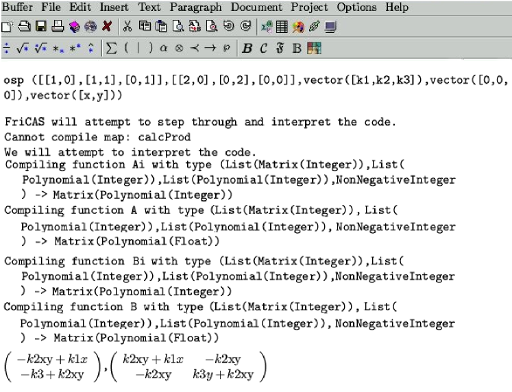
osp ([[1,0],[1,1],[0,1]],[[2,0],[0,2],[0,0]],
        vector([k1,k2,k3]), vector([0,0,0]),
               vector([x,y]))

Fig. 1 represents the result obtained in TeXmacs shell. In fact, we repeated the results obtained in (19).

Figure 1: The output of the module for predator–prey model in graphic TeXmacs shell

VI Numerical experiment for the program complex

VI.1 Stochastic Runge–Kutta methods

Euler–Maruyama method is one of well-known numerical methods for solving SDE, it is a special case of a more general Stochastic Runge–Kutta method. Classical Runge–Kutta method can be generalized to the case of the SDE system (10) in the following manner Debrabant and Röbler (2008); Tocino and Ardanuy (2002):

$$\left\{\begin{aligned} X^{i}_{k}=&x_{0}^{i}+hR^{\underline{\vphantom{j}{l}}}_{k}a^{i}(X^{1}_{\underline{\vphantom{j}{l}}},\ldots,X^{n}_{\underline{\vphantom{j}{l}}})+\widehat{R}^{\underline{\vphantom{j}{l}}}_{k}J^{\alpha}b^{i}_{\alpha}(X^{1}_{\underline{\vphantom{j}{l}}},\ldots,X^{n}_{\underline{\vphantom{j}{l}}}),\\ x^{i}_{1}=&x_{0}^{i}+hr^{\underline{\vphantom{j}{l}}}a^{i}(X^{1}_{\underline{\vphantom{j}{l}}},\ldots,X^{n}_{\underline{\vphantom{j}{l}}})+\hat{r}^{\underline{\vphantom{j}{l}}}J^{\alpha}b^{i}_{\alpha}(X^{1}_{\underline{\vphantom{j}{l}}},\ldots,X^{n}_{\underline{\vphantom{j}{l}}})\end{aligned}\right.$$ (21)

Indexes $k=1,\ldots,s$ and $l=1,\ldots,n$ refer to stochastic Runge–Kutta method. $J\sim N(0,h)$ or $J\sim\sqrt{h}\varepsilon$, $\varepsilon\sim N(0,1)$ are normal distributed random variables. Such a choice of these numerical values for approximation is made because the Wiener process is implemented as $\mathrm{d}W=\varepsilon\sqrt{\mathrm{d}t}$. You should also pay attention to double summation in the third term of both numerical scheme formulas as well as the fact that each number $J^{1},\ldots,J^{n}$ should generated separately.

The method coefficients, as well as for the classical analogue, can be grouped into a table called the Butcher table:

$$\begin{array}[]{c|c|c}&R_{ij}&\hat{R}_{ij}\\ \hline\cr&r_{j}&\hat{r}_{j}\end{array}.$$ (22)

For calculations we used a method with the table

$$\begin{array}[]{c|ccc|ccc}&0&0&0&0&0&0\\ &2/3&0&0&2/3&0&0\\ &-1&1&0&-1&1&0\\ \hline\cr&0&3/4&1/4&0&3/4&1/4\end{array}$$ (23)

VI.2 Software implementation description

The purposes of the programs complex were to automate the SDE coefficients $A^{i}$ and $B^{ij}$ computation with the help of general principles described above, and to find a numerical solution of the equation obtained by means of stochastic Runge–Kutta methods. From a programming standpoint we can derive three subtasks:

1. coefficients $A^{i}$ and $B^{ij}$ generation using the computer algebra system;

2. generation of source code in languages Fortran and Julia, implementing the SDE on the basis of the coefficients, saved as a text file;

3. writing subroutines/functions implementing stochastic Runge–Kutta methods in Fortran and Julia, and their subsequent compilation together with automatically generated source codes.

As a result of its work Axiom module creates a text file which contains the coefficients $A^{i}$ and $B^{ij}$ in the following form:

        # A
        A[1]
        ...
        A[N]
        # B
        B[1,1] B[1,2] .. B[1,N]
        ...
        B[N,1] B[N,2] .. B[N,N]

Matrix $b^{i}_{\alpha}=\sqrt{b^{i}_{\alpha}b^{j\alpha}}=\sqrt{B^{ij}}$ is calculated numerically with the help of the singular value matrix decomposition (a subroutine DGESVD from library LAPACK is used).

For the second subtask scripting language Python was chosen (version 3). This language has a wide set of tools to work with strings and text files. Except matrices $A^{i}$ and $B^{ij}$ additional information about the mathematical model was specified as dictionary (standard data type in Python), with model name, list of variables, list of parameters, initial values of variables, parameters values and parameters of the numerical method (integration section and step size).

On the basis of these data, the script automatically generates two files functions.f90 and main.f90, where the first is a module with functions defining the SDE, and the second one is a main program file. While compiling these files the third additional module with auxiliary procedures with Stochastic Runge–Kutta method is added.

VI.3 The numerical experiment description

For the programs complex work verification a well-known predator–prey model was chosen with vector $a^{i}$ components

$$a^{1}=\alpha x-\beta xy,\;\;a^{2}=-\gamma y+\delta xy$$ (24)

and matix $B^{ij}$:

$$\left[\begin{array}[]{cc}\alpha x+\beta xy&-\beta xy\\ -\beta xy&\beta xy+\gamma x\end{array}\right],$$ (25)

$x$ is the number of preys, $y$ is the number of predators. Coefficients also have the following physical (biological) meaning: $\alpha$ is the growth rate of the prey population, $\beta$ is a frequency of predators and prey meetings, $\gamma$ is an intensity of predators death or migration in a lack of preys, $\delta$ is a predator population growth rate on the assumption of the excess of the prey.

During numerical simulations it was taken into account that the value of variables $x,y$ could not be less than zero (program stop working when one of the variables becomes equal to zero).

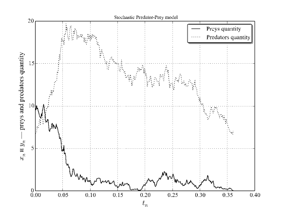
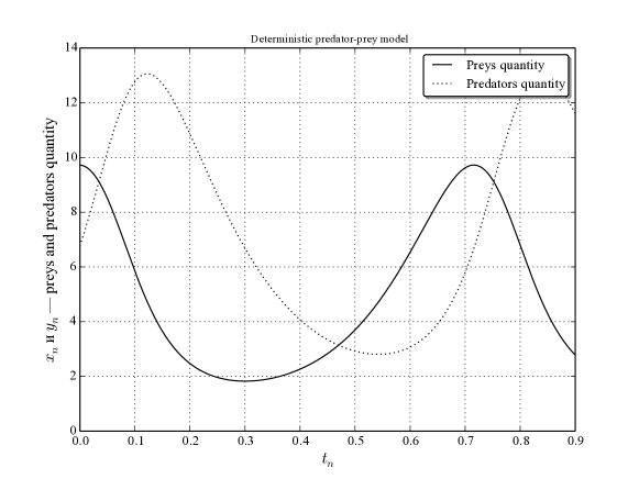
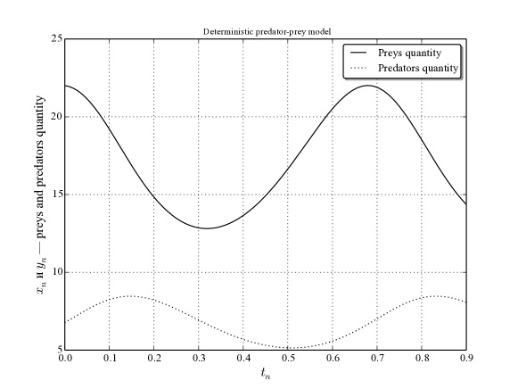
Numerical simulation shows that the addition of stochastic to the classical predator–prey model leads to the fact that after a certain time death of one of the competing species comes. So, for the following parameters: $\alpha=10$, $\beta=1,5$, $\gamma=8,5$, $\delta=1,8$ and the initial values: $x=9,7$, $x=6,77$, victims are first to die, and after that predators die due to lack. This case is illustrated in Fig. 2. For comparison in Fig. 3 is a graph for the deterministic case .

Figure 2: Stochastic predator–prey model, prey die

Figure 3: Deterministic predator–prey model

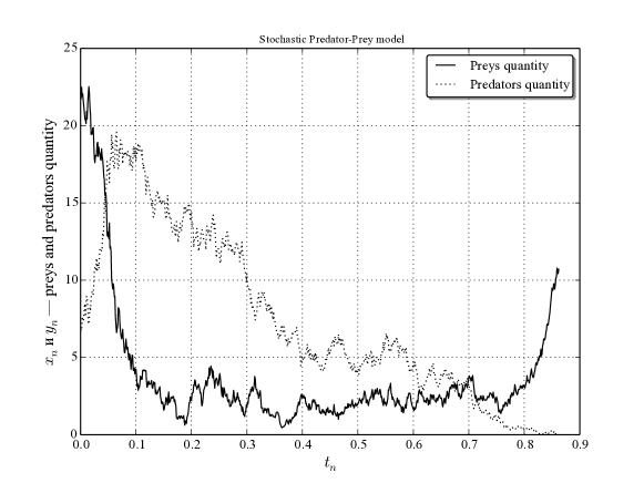
Under other conditions ($\alpha=10$, $\beta=1,5$, $\gamma=8,5$, $\delta=0,5$, $x=22$, $y=6,76$) predators die, and the number of victims is increasing rapidly, as for their model assumes an infinite source of food. Graphics for this case are shown in Fig. 4, and Fig. 5 shown for comparison with deterministic case.

Figure 4: Stochastic predator–prey model, predators die

Figure 5: Deterministic predator–prey model

VII Conclusions

This work demonstrates the application of the developed initial physical system formalization method. The system is presented in the form of one or more one-step processes. Formalization of the system is done by introducing the evolution operator. Wherein the analytical description of the model requires a lot of routine operations. To simplify the work we propose to use the computer algebra system (Axiom fork FriCAS).

We have developed an analytical software package block that receives inlet evolution operator and produces the SDE, which describes the original model. For numerical studies of obtained SDE system a second software unit that converts the resulting system of equations into the program code in fortran and gives its numerical solution was developed. Thus, the software system is applicable for both analytical and numerical study of the original model.

Currently the software package does not cover all possibilities, incorporated in the proposed method of formalizing the original physical system. Since the original system description uses ODE, we should introduce the boundary conditions by ties or indicator functions. Partial differential equations can help to solve this problem. Further objective is the development of a complete software complex for a method of one-step original physical system model construction.

References

- Demidova and Kulyabov [2012] A. V. Demidova and D. S. Kulyabov. The Introduction of an Agreed Term in the Equation of Stochastic Population Model. Bulletin of Peoples Friendship University of Russia. Series Mathematics. Information Sciences. Physics, (3):69–78, 2012. In Russian.
- Demidova et al. [2010] Anastsasiya Vyacheslavovna Demidova, Leonid Antonovich Sevastianov, and Dmitry Sergeevich Kulyabov. Application of Stochastic Differencial Equations to Model Population Systems. In Third International Conference on Mathematical Modelling of Social and Economical Dynamics MMSED-2010, pages 92–94. Russian State Social University, 2010. In Russian.
- Debrabant and Röbler [2008] Kristian Debrabant and Andreas Röbler. Classification of Stochastic Runge–Kutta Methods for the Weak Approximation of Stochastic Differential Equations. Mathematics and Computers in Simulation, 77(4):408–420, 2008. ISSN 0378-4754. doi: http://dx.doi.org/10.1016/j.matcom.2007.04.016.
- Tocino and Ardanuy [2002] A. Tocino and R. Ardanuy. Runge–Kutta Methods for Numerical Solution of Stochastic Differential Equations. Journal of Computational and Applied Mathematics, 138(2):219–241, 2002. ISSN 0377-0427. doi: http://dx.doi.org/10.1016/S0377-0427(01)00380-6. URL http://www.sciencedirect.com/science/article/pii/S0377042701003806.
- Volterra [1976] Vito Volterra. Mathematical Theory of the Struggle for Existence. Nauka, 1976.
- Bazykin [1998] A. D. Bazykin. Nonlinear Dynamics of Interacting Populations. World Scientific, 1998.
- Bratus et al. [2010] A. S. Bratus, A. S. Novozhilov, and A. P. Platonov. Dynamical systems and biology models. Fizmatlit, M., 2010. In Russian.
- Penrose and Rindler [1984] Roger Penrose and Wolfgang Rindler. Spinors and Space-Time: Two-Spinor Calculus and Relativistic Fields, volume 1. Cambridge University Press, 1984.
- Demidova et al. [2014] A. V. Demidova, M. N. Gevorkyan, A. D. Egorov, A. V. Korolkova, D. S. Kulyabov, and L. A. Sevastyanov. Influence of stochastization to one-step model. Bulletin of Peoples’ Friendship University of Russia. Series Mathematics. Information Sciences. Physics, (1):71–85, 2014. In Russian.
- Demidova et al. [2013] Anastsasiya Vyacheslavovna Demidova, Anna Vladislavovna Korolkova, Dmitry Sergeevich Kulyabov, and Leonid Antonovich Sevastianov. The Method of Stochastization of One-Step Processes. In Mathematical Modeling and Computational Physics, page 67. JINR, 2013.
- Gardiner [1985] C. W. Gardiner. Handbook of Stochastic Methods: for Physics, Chemistry and the Natural Sciences. Springer Series in Synergetics, 1985.
- Øksendal [2003] B. K. Øksendal. Stochastic Differential Equations: An Introduction with Applications. Springer, Berlin, 2003.
- Lotka [2011] A. J. Lotka. Elements of Physical Biology. BiblioBazaar, 2011. ISBN 9781178508116. URL http://books.google.ru/books?id=tFN9pwAACAAJ.
- Demidova [2013a] A. V. Demidova. The Equations of Population Dynamics in the Form of Stochastic Differential Equations. Bulletin of Peoples’ Friendship University of Russia. Series Mathematics. Information Sciences. Physics, (1):67–76, 2013a. In Russian.
- Demidova [2013b] A. V. Demidova. The method of stochastization of mathematical models for the example of the ‘‘predator–prey’’. In A Scientific Session NRNU MEPHI-2013, page 127, 2013b. In Russian.
- Korolkova [2013] Kulyabov D. S. Korolkova, A. V. Methods of Stochastization of Mathematical Models on the Example of Peer to Peer Networks. In A Scientific Session NRNU MEPHI-2013, page 131, Moscow, 2013. MEPHI. In Russian.
- Demidova et al. [2012] Anastsasiya Vyacheslavovna Demidova, Dmitry Sergeevich Kulyabov, and Leonid Antonovich Sevastianov. The agreed stochastic term in population models. In XI Belarusian Mathematical Conference, page 39, Minsk, 2012. Institute of Mathematics of the National Academy of Sciences of Belarus. In Russian.