A Bayesian Approach to Sparse plus Low rank Network Identification

Abstract

We consider the problem of modeling multivariate stochastic processes with parsimonious dynamical models which can be represented with a sparse dynamic network with few latent nodes. This structure translates into a sparse plus low rank model. In this paper, we propose a Bayesian approach to identify such models.

I INTRODUCTION

This paper deals with the network identification problem of a multivariate stochastic process of high dimension. Important applications can be found in many fields, for instance in econometrics, [1, 5, 8, 21], social network analysis [13], system biology, [20] and so on.

Let $y$ be a stochastic process whose components (or variables) $y_{k}$ are manifest, i.e. can be directly measured. We define as network of this manifest process $y$ a directed graph wherein nodes denote the variables and edges encode conditional Granger causality relations among these variables, [12]. More specifically, there is an edge from node $i$ (i.e. variable $y_{i}$) to node $j$ (i.e. variable $y_{j}$) if the past of $y_{i}$ is needed to predict $y_{j}$ conditioned on the past of all the other $y_{k}$, $k\neq i$. Sparse graphs (i.e. with few edges) represent a concise and interpretable way to describe the relations among the variables of the manifest process, [7]. However, this modeling assumption does not exploit nor encode the fact that the manifest process may often be thought as driven by a low dimensional latent process, i.e. a stochastic process whose components cannot be directly measured.

In this paper we formulate a new network identification problem which takes into account the presence of this low dimensional latent process and the variables of the manifest process Granger causes each other mostly through the latent variables. The corresponding network has a two layer structure: one layer denotes the manifest variables and the other one the latent variables. The presence of few latent variables should drastically reduce the edges in the manifest layer, therefore increasing the degree of conciseness and robustness of the model. Finally, it turns out that a model described by this network has a sparse plus low rank (S+L) structure. More precisely, the low rank part depends on the number of latent variables, whereas the sparse one on the number of conditional Granger causality relations among the manifest variables.

When it comes to developing and identification algorithm, which maps measured data into an estimated dynamical model, it is fair to say that the prediction error method (PEM) is a consolidate paradigm in system identification [15, 19]. In the traditional setting, candidate models are described in fixed parametric model structures, e.g. ARMAX, whose complexity is determined using cross validation or information based criteria. Regularization has been recently introduced in the PEM framework, see [16, 17, 6, 18], as an alternative approach to control complexity of the estimated models. This latter class of methods start with a large enough (in principle infinite dimensional) model class; the inverse (ill-posed) problem of determining a specific model from a finite set of measured data can be made into a well posed problem using a penalty term, whose duty is to select models with specific features. In the Bayesian view, this is equivalent to the introduction of an a priori probability (i.e. prior) on the model to estimate. For instance, the prior should account the fact that the model is Bounded Input Bounded Output (BIBO) stable, [17].

The identification algorithm we propose belongs to this latter class of methods, where the predictor impulse response is estimated in the framework of Gaussian regression. The predictor impulse response is modeled as a zero mean Gaussian random vector. Its covariance matrix, referred to as kernel matrix, encodes the a priori information. In this case, the a priori information is that the predictor impulse responses are BIBO stable and that the model has a S+L structure. As we will see, such a priori information can be encoded in the kernel matrix using the maximum entropy principle. Moreover, this kernel matrix is characterized by the decay rate of the predictor impulse responses, by the number of conditional Granger causality relations among the manifest variables, and by the number of latent variables. These features are tuned by the so called hyperparameters vector. It is estimated by minimizing the negative log-likelihood of the measured data. Beside the fact that this problem is nonconvex, the joint estimation of the hyperparameters tuning the sparse and low rank part is not trivial, because these two parts may be nonidentifiable from the measured data. We propose an algorithm to estimate these hyperparameters which imposes and “hyper-regularizer” on the low rank hyperparameter to handle partially this non-uniqueness. Once the kernel matrix is fixed, an unique estimate of the S+L model is guaranteed through regularization.

We warn the reader that the present paper only reports some preliminary result regarding the Bayesian estimation of S+L models. In particular, all the proofs and most of the technical assumptions needed therein are omitted and will be published afterwards.

The outline of the paper follows. In Section II, we introduce the S+L model for multivariate stochastic processes. In Section III, we apply the Gaussian approach to S+L system identification. In Section IV, we derive the kernel matrix by the maximum entropy principle. In Section V, we present the algorithm to estimate the hyperparameters of the kernel matrix. In Section VI, we provide some numerical examples to show the effectiveness of our method. Finally, the conclusions are in Section VII.

Notation

Throughout the paper, we will use the following notation. $\mathcal{S}_{m}^{+}$ denotes the cone of the positive definite symmetric matrices, and $\overline{\mathcal{S}}_{m}^{+}$ its closure. Given $v\in\mathbb{R}^{m}$ and $G\in\mathbb{R}^{n\times m}$, $v_{i}$ denotes the $i$-th entry of $v$ and $[G]_{ij}$ denotes the entry of $G$ in position $(i,j)$. $\|G\|_{Q}$ denotes the weighted Frobenius norm of $G$ with weight matrix $Q\in\mathcal{S}_{m}^{+}$. Given a transfer matrix $L(z)$ of dimension $m\times m$, with some abuse of terminology, we say that $L(z)$ has rank equal to $n$, with $n\leq m$, if it admits the decomposition $L(z)=FH(z)$ where $F\in\mathbb{R}^{m\times n}$ and $H(z)$ is a $n\times m$ transfer matrix. Given a stochastic process $y=\{y(t)\}_{t\in\mathbb{Z}}$, with some abuse of notation, $y(t)$ will both denote a random vector and its sample value. Finally,

$$\mathrm{y}^{-}(t):=\left[\begin{array}[]{ccc}y(t-1)^{\top}&y(t-2)^{\top}&\ldots\\ \end{array}\right]^{\top}$$ (1)

denotes the past data vector of $y$ at time $t$. In similar way, $\mathrm{y}_{i}^{-}(t)$ denotes the past data vector of $y_{i}$.

II S+L Models

Consider two zero mean stationary Gaussian stochastic processes $y$ and $x$ of dimension $m$ and $n$, respectively. Let $y$ be manifest, i.e. it can be measured, and $x$ latent, i.e. it cannot be measured. We assume that $y(t)\in\mathbb{R}^{m}$ and $x(t)\in\mathbb{R}^{n}$ are described by the model

$$y(t) = Fx(t)+S(z)y(t)+v(t)$$

$$x(t) = H(z)y(t)+w(t)$$ (2)

where $H(z)=\sum_{k=1}^{\infty}H_{k}z^{-k}$ is a BIBO stable transfer matrix of dimension $n\times m$, $F\in\mathbb{R}^{m\times n}$, $S(z)=\sum_{k=1}^{\infty}S_{k}z^{-k}$ is a BIBO stable transfer matrix of dimension $m\times m$, $v$ and $w$ are, respectively, $m$ and $n$ dimensional white Gaussian noise (WGN) with zero mean, and covariance matrix $\Sigma_{v}$ and $\Sigma_{w}$. Moreover, $v$ and $w$ are independent.

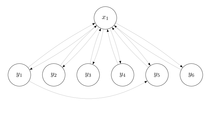
It is possible to describe the structure of model (II) using a directed graph (i.e. network) as in Figure 1, [14]. Each node of this network corresponds to components of $y$ or $x$; edges encode conditional Granger causality relations. More precisely, there is a direct link from node $y_{j}$ ($x_{j}$) to node $y_{i}$ ($x_{i}$) if and only if $\mathrm{y}_{j}^{-}(t)$ ($x_{j}(t)$) is needed to predict $y_{i}(t)$ ($x_{i}(t)$), conditionally on all the past information available at time $t$, i.e. $\mathrm{y}_{k}^{-}(t)$ with $k\neq j$ and $x(t)$ ($\mathrm{y}^{-}(t)$ and $x_{k}(t)$ with $k\neq j$). In this case, we shall say that $y_{j}$ ($x_{j}$) conditionally Granger causes $y_{i}$ ($x_{i}$), [12]. In Figure 1 we provide an example with $m=6$ and $n=1$. In particular, $x_{1}$ conditionally Granger causes all the components in $y$ and conversely, and $y_{1}$ conditionally Granger causes $y_{5}$.

Figure 1: Example of a sparse plus low rank model with $m=6$ and $n=1$.

Our main modeling assumption in (II) is that manifest variables Granger cause each other mostly through few latent variables. Therefore, we have $n\ll m$, i.e. the number of latent variables in $x$ is small as compared to the number of manifest variables in $y$; similarly $S(z)$ is sparse, i.e. many of its entries are null transfer functions, so that few manifest variables conditionally Granger causes each other. From (II), we obtain the sparse plus low rank (S+L) model for $y$:

$$y(t)=S(z)y(t)+L(z)y(t)+e(t)$$ (3)

where $S(z)$ is a sparse transfer matrix by assumption, $L(z):=FH(z)$ is a low rank transfer matrix because $F$ and $H^{\top}(z)$ are tall matrices, and $e(t):=v(t)+w(t)$ is WGN with covariance matrix $\Sigma=\Sigma_{v}+F\Sigma_{w}F^{\top}$.

Let $\hat{y}(t|t-1)$ be the minimum variance one-step ahead predictor of $y(t)$ based on the observations $\mathrm{y}^{-}(t)$, and $\hat{x}(t|t-1)$ be the minimum variance estimator of $x(t)$ based on $\mathrm{y}^{-}(t)$. From (II), we have

$$\hat{y}(t|t-1) = F\hat{x}(t|t-1)+S(z)y(t)$$

$$\hat{x}(t|t-1) = H(z)y(t).$$ (4)

that is, the predictable part of $y$ is a function of few estimated latent variables and of the pasts of few manifest variables of $y$. Eq. (II) can be compactly written as

$$\begin{array}[]{rcl}\hat{y}(t|t-1)&=&S(z)y(t)+L(z)y(t).\end{array}$$ (5)

It is worth noting that in the case that $L(z)=0$, i.e. there is no need of latent variables to characterize the predictor of $y$, we obtain the sparse model presented in [7]. In the case $S(z)=0$, i.e. the predictor of $y$ is completely characterized by the estimators of the latent variables, we obtain a quasi-static factor model where the noise process is white, see for instance [10]. We would like to stress that the decomposition of a transfer matrix into sparse plus low rank may not be unique. As noticed in [5], this degeneracy may occur when $L(z)$ is sparse or $S(z)$ has few null entries. Although this nonidentifiability issue is important, the aim of this paper is to find one S+L decomposition (see Section III) which is not necessarily unique.

III Gaussian Regression Approach to System Identification

Consider model (II) and assume that the measured data $y(1)\ldots y(N)$ are extracted from a realization of $y$. The latent process $x$ cannot be measured nor its dimension $n$ is known. In this Section, we address the problem of estimating $S(z)$ and $L(z)$ from the given data. We draw inspiration from the Gaussian regression approach proposed in [16]. According this method, $y$ is generated by model

$$y(t)=G(z)y(t)+e(t)$$ (6)

where $G(z)$ is a BIBO stable $m\times m$ transfer matrix and $e$ is WGN with covariance matrix $\Sigma$. Note that, if we set $G(z)=S(z)+L(z)$ then (6) is equivalent to (3). On the other hand, with (6) we loose the S+L structure we are interest in.

Since $G(z)$ is BIBO stable, and thus the impulse response coefficients decay to zero as a function of the lag index, it is possible to use the approximation

$$G(z)=\sum_{k=1}^{T}G_{k}z^{-k}$$ (7)

where $T$ is sufficiently large. The parameters $G_{k}$, $k=1,.,T$ of the truncated transfer matrix are stacked in the vector $\theta\in\mathbb{R}^{m^{2}T}$ which is defined as follows

$$\theta = \left[\begin{array}[]{ccc|c}(g^{[11]})^{\top}&\ldots&(g^{[1m]})^{\top}&\ldots\\ \end{array}\right.$$ (11)

$$\hskip 5.69046pt\left.\begin{array}[]{c|ccc}\ldots&(g^{[m1]})^{\top}&\ldots&(g^{[mm]})^{\top}\\ \end{array}\right]^{\top}$$

where

$$g^{[ij]}=\left[\begin{array}[]{cccc}[G_{1}]_{ij}&[G_{2}]_{ij}&\ldots&[G_{T}]_{ij}\\ \end{array}\right]^{\top}$$ (12)

denotes the impulse response coefficients of the transfer function in position $(i,j)$ of the truncated approximation of $G(z)$. Then, we stack the measured data in the vector $\mathrm{y}$ as follows

$$\mathrm{y} = \left[\begin{array}[]{ccc|c}y_{1}(T+1)^{\top}&\ldots&y_{1}(N)^{\top}&\ldots\\ \end{array}\right.$$ (16)

$$\hskip 5.69046pt\left.\begin{array}[]{c|ccc}\ldots&y_{m}(T+1)^{\top}&\ldots&y_{m}(N)^{\top}\\ \end{array}\right]^{\top}.$$

In similar way, we define

$$\mathrm{e} = \left[\begin{array}[]{ccc|c}e_{1}(T+1)^{\top}&\ldots&e_{1}(N)^{\top}&\ldots\\ \end{array}\right.$$ (20)

$$\hskip 5.69046pt\left.\begin{array}[]{c|ccc}\ldots&e_{m}(T+1)^{\top}&\ldots&e_{m}(N)^{\top}\\ \end{array}\right]^{\top}.$$

From (6) the vector of the measured data can be expressed in the linear regression form

$$\mathrm{y}=\Phi\theta+\mathrm{e}$$ (21)

where $\Phi\in\mathbb{R}^{mN\times m^{2}T}$ is the regression matrix. Note that, $\Phi\theta$ is the one-step ahead predictor of $\mathrm{y}$.

According to the Gaussian regression framework, $\theta$ is modeled as a zero mean Gaussian random vector with covariance matrix, or kernel matrix, denoted by $K\in\mathcal{S}_{m^{2}T}^{+}$.

Let $\hat{\theta}$ be the posterior mean of $\theta$ given $\mathrm{y}$. In [16] it has been proved that, under some technical assumption, $\hat{\theta}$ can also be written as solution to the Tikhonov regularization problem

$$\hat{\theta}=\underset{\begin{subarray}{c}\theta\end{subarray}}{\arg\min}\|\mathrm{y}-\Phi\theta\|^{2}_{\Sigma^{-1}\otimes I_{N}}+\|\theta\|^{2}_{K^{-1}}.$$ (22)

Moreover, it is not difficult to see that

$$\hat{\theta}=K\Phi^{\top}(\Phi K\Phi^{\top}+\Sigma\otimes I_{N})^{-1}\mathrm{y}.$$ (23)

Remark III.1

Using the theory of reproducing kernel Hilbert spaces, [3], it is possible to show that the above results still hold for $T\rightarrow\infty$, [16].

Remark III.2

Although we assumed $K\in\mathcal{S}_{m^{2}T}^{+}$, the Bayes estimator (23) also holds for $K$ singular. In that case, Problem (22) is well defined provided that $\theta$ belongs to the range of $K$.

The optimal solution $\hat{\theta}$ highly depends on the choice of $K$. A typical assumption is that the transfer functions in $G(z)$ are independent, that is $g^{[ij]}$ are independent vectors. We shall also assume that $g^{[ij]}$, with $i,j=1\ldots m$, are identically distributed, so that $K=I_{m^{2}}\otimes\tilde{K}$ where $\tilde{K}\in\mathcal{S}_{T}^{+}$ is the covariance matrix of $g^{[ij]}$, with $i,j=1\ldots m$. In this paper, $\tilde{K}$ is chosen as a filtered version of the tuned/correlated (TC) kernel, see [16] and [6] for more details. It is important to note this kernel is able to capture high frequency oscillations, which are typical of the predictor impulse responses for low pass processes, and enforces BIBO stability as $T\rightarrow\infty$ on the posterior mean of the predictor impulse responses.

III-A Gaussian Regression Approach to S+L Identification

The idea is to model $S(z)$ and $L(z)$ through Gaussian process, similarly to what has been done above for $G(z)$. In particular, since $S(z)$ and $L(z)$ are BIBO stable, we can consider their truncated approximations with $T$ is sufficiently large. Then, it is not difficult to see that

$$\mathrm{y}=\Phi(\theta_{l}+\theta_{s})+\mathrm{e}$$ (24)

where $\mathrm{y}$ and $\mathrm{e}$ have been defined in (16) and (20). $\theta_{s},\theta_{l}\in\mathbb{R}^{m^{2}T}$ contains the parameters of the truncated approximations of $S(z)$ and $L(z)$, respectively. Then, we model $\theta_{s}$ and $\theta_{l}$ as zero mean random vectors with covariance matrix $K_{S}$ and $K_{L}$, respectively. Moreover, we shall assume that $\theta_{s}$ and $\theta_{l}$ are Gaussian and independent. As we will see in Section IV, these assumptions are suggested by the maximum entropy principle.

Proposition III.1

Let $\hat{\theta}_{s}$ and $\hat{\theta}_{l}$ be, respectively, the posterior mean of $\theta_{s}$ and $\theta_{l}$ given $\mathrm{y}$. Then, under some technical assumption, $\hat{\theta}_{s}$ and $\hat{\theta}_{l}$ are solution to the Tikhonov regularization problem

$$\underset{\begin{subarray}{c}\theta_{s},\theta_{l}\end{subarray}}{\arg\min}\|\mathrm{y}-\Phi(\theta_{s}+\theta_{l})\|^{2}_{\Sigma^{-1}\otimes I_{N}}+\|\theta_{s}\|^{2}_{K_{S}^{-1}}+\|\theta_{l}\|^{2}_{K_{L}^{-1}}.$$ (25)

Moreover, we have

$$\hat{\theta}_{s}=K_{S}\Phi^{\top}c,\;\;\hat{\theta}_{l}=K_{L}\Phi^{\top}c$$ (26)

where

$$c=(\Phi(K_{S}+K_{L})\Phi^{\top}+\Sigma\otimes I_{N})^{-1}\mathrm{y}.$$ (27)

In what follows, $\hat{\theta}_{s}$ and $\hat{\theta}_{l}$ will be referred to as posterior mean of $S(z)$ and $L(z)$, respectively. In the next Section, we shall show how $K_{S}$ and $K_{L}$ can be chosen so as to enforce BIBO stability on both the posterior mean of $S(z)$ and $L(z)$, sparsity on the posterior mean of $S(z)$ as well as low rank of the posterior mean of $L(z)$.

IV Maximum Entropy Kernel Matrix

In this Section we characterize the prior probability density of $\theta_{s}$ and $\theta_{l}$ by using the maximum entropy principle. Such principle states that among all the prior probability densities satisfying certain desired constraints, the optimal one should maximize the differential entropy.

Our starting assumptions are that $\theta_{s}$ and $\theta_{l}$ are absolutely continuous zero mean random vectors. Let $\mathbf{p}(\theta_{s},\theta_{l})$ denote the joint probability density of $\theta_{s}$ and $\theta_{l}$. Let $\mathbb{E}$ denote the integration over $\mathbb{R}^{2m^{2}T}$ with respect to the probability measure $\mathbf{p}$. Moreover, $\mathcal{P}$ denotes the space of probability densities which are Lebesgue integrable. The differential entropy of $\mathbf{p}\in\mathcal{P}$ is, [9],

$$\mathbf{H}(\mathbf{p})=-\mathbb{E}[\log(\mathbf{p}(\theta_{s},\theta_{l}))].$$ (28)

Next, we characterize the constraint on $\theta_{s}$ enforcing BIBO stability and sparsity on the posterior mean of $S(z)$. The transfer function in position $(i,j)$ of $S(z)$ is the null transfer function if and only if $s^{[ij]}$ is the null vector. We consider the constraint

$$\mathbb{E}[\|s^{[ij]}\|^{2}_{\tilde{K}^{-1}}]\leq p_{ij},$$ (29)

where $p_{ij}\geq 0$. If $p_{ij}=0$, then $s^{[ij]}$ is zero in mean square and so also is its posterior mean. Moreover, simple algebraic manipulations show that the weighted second moment bound in (29) implies a bound on the variance of $k$-th element of $s^{[ij]}$ which decays as the $k$-th element in the main diagonal of $\tilde{K}$. Therefore, condition (29) enforces BIBO stability and sparsity on the posterior mean of $S(z)$.

Regarding the low rank constraint on $\theta_{l}$, let $A_{l}\in\mathbb{R}^{m\times mT}$ be the random matrix such that

$$A_{l}=\left[\begin{array}[]{cccc}L_{1}&L_{2}&\ldots&L_{T}\end{array}\right].$$ (30)

Consider the constraint

$$\mathbb{E}[A_{l}(\tilde{K}^{-1}\otimes I_{m})A_{l}^{\top}]\leq Q.$$ (31)

If $Q\in\overline{\mathcal{S}}_{m}^{+}$ has $m-n$ singular values equal to zero, then the posterior mean of $A_{l}A_{l}^{\top}$ has rank less than or equal to $n$. Therefore, the latter admits the decomposition

$$A_{l}=\left[\begin{array}[]{cccc}FH_{1}&FH_{2}&\ldots&FH_{T}\end{array}\right],$$ (32)

where $F\in\mathbb{R}^{m\times n}$ and $H_{k}\in\mathbb{R}^{n\times m}$, $k=1\ldots T$, as in Section II. Equivalently, the posterior mean of $L(z)$ admits the decomposition $L(z)=FH(z)$. Similarly to the sparse part, the weight matrix $\tilde{K}^{-1}\otimes I_{m}$ enforces BIBO stability on the posterior mean of $L(z)$.

Consider the following maximum entropy problem

$$\underset{\mathbf{p}\in\mathcal{P}}{\max} \mathbf{H}(\mathbf{p})$$ (33)

s.t. $$\mathbb{E}[\|s^{[ij]}\|^{2}_{\tilde{K}^{-1}}]\leq p_{ij}\;\;i,j=1\ldots m$$

$$\mathbb{E}[A_{l}(\tilde{K}^{-1}\otimes I_{m})A_{l}^{\top}]\leq Q$$

where $p_{ij}>0$ $i,j=1\ldots m$, and $Q\in{\mathcal{S}}_{m}^{+}$.

Theorem IV.1

The optimal solution to (33) is such that $\theta_{s}$ and $\theta_{l}$ are independent, Gaussian with zero mean and covariance matrix

$$K_{S}=\Gamma\otimes\tilde{K},\;\;K_{L}=\Lambda\otimes I_{m}\otimes\tilde{K}$$ (34)

where

$$\Gamma=\mathrm{diag}(\gamma_{11}\ldots\gamma_{m^{2}})\in\mathcal{S}_{m^{2}}^{+}$$ (35)

and $\Lambda\in\mathcal{S}_{m}^{+}$.

The matrices $\Gamma$ and $\Lambda$ are the hyperparameters of the kernel matrices $K_{S}$ and $K_{L}$, respectively. Clearly, we are interested in the limiting case where $p_{ij}=0$ for some $(i,j)$ and $Q$ low-rank. Let $\mathbf{P}=\{(i,j)\hbox{ s.t }p_{ij}=0\}$ and $\mathbf{Q}=\{v\in\mathbb{R}^{m}\hbox{ s.t }Qv=0\}$. Then, it can be shown that the maximum entropy solution can be extended by continuity to this limiting case where $\gamma_{(i-1)m+j}=0$ if and only if $(i,j)\in\mathbf{P}$ and $\Lambda v=0$ if and only if $v\in\mathbf{Q}$. Thus, $\Gamma$ tunes sparsity on the posterior mean of $S(z)$ and $\Lambda$ tunes the rank on the posterior mean of $L(z)$. Finally, is worth noting that the hyperparameters tuning the decay rate of the posterior mean of the predictor impulse responses are encoded in $\tilde{K}$, [17].

V Estimation of the Hyperparameters

In order to compute $\hat{\theta}_{s}$ and $\hat{\theta}_{s}$ we need to estimate the hyperparameters in $\tilde{K}$ and the matrices $\Gamma$ and $\Lambda$. The hyperparameters describing $\tilde{K}$ are estimated in a preliminary step by minimizing the negative log-likelihood of model (6), see [16]. $\Gamma$ and $\Lambda$ are obtained minimizing the negative log-marginal likelihood $\ell$ of $\mathrm{y}$. Under some technical assumption, we have, [16],

$$\ell(\mathrm{y},\Gamma,\Lambda)=\frac{1}{2}\log\det V+\frac{1}{2}\mathrm{y}^{\top}V^{-1}\mathrm{y}+\mathrm{const.term}$$ (36)

where

$$V=\Phi(K_{S}+K_{L})\Phi^{\top}+\Sigma\otimes I_{N}.$$ (37)

Since (36) is nonconvex in $V$, only local minima can be computed. Beside that, the joint minimization of $\Gamma$ and $\Lambda$ is not trivial because the sparse and low rank part may be nonidentifiable from the measured data. For this reason, we constrain the structure of $\Lambda$ as follows:

$$\Lambda=\alpha(I-UU^{\top})+U\mathrm{diag}(\beta_{1}\ldots\beta_{r})U^{\top}$$ (38)

where $U\in\mathbb{R}^{m\times r}$ and its columns are the first $r$ singular vectors of an estimate $\hat{A}_{l}\hat{A}_{l}^{\top}$ of $A_{l}A_{l}^{\top}$. In this way, the constraints in $\Lambda$ are decoupled along the “most reliable” $r$ singular vectors of $\hat{A}_{l}\hat{A}_{l}^{\top}$ and their orthogonal complement. This is equivalent to fix $r$ latent variables (from the estimate $\hat{A}_{l}\hat{A}_{l}^{\top}$). Regarding the hyperparameter $\Gamma$, in [2] it has been shown that the minimization of (36) leads sparsity in the main diagonal of $\Gamma$. Therefore, we minimize (36) with respect to $\tilde{\xi}=\{\gamma_{1}\ldots\gamma_{m^{2}},\alpha,\beta_{1}\ldots\beta_{r}\}$ while $r$ and $U$ are fixed. The complete procedure to estimate $r$, $U$ and $\tilde{\xi}$ is described in Algorithm 1. $r^{(k)}$, $U^{(k)}$, $\hat{A}_{l}^{(k)}$ and $\tilde{\xi}^{(k)}$ denote, respectively, $r$, $U$, $\hat{A}_{l}$ and $\tilde{\xi}$ at the $k$-th iteration. Finally, to minimize efficiently (36) with respect to $\tilde{\xi}$ we used the scaled gradient projection algorithm developed in [4].

Algorithm 1 Computation of $r$, $U$ and $\tilde{\xi}$

1:$k=0$

2:$r^{(0)}\leftarrow 0$

3:$U_{OPT}^{(0)}\leftarrow$ empty matrix

4:$\tilde{\xi}^{(0)}\leftarrow\underset{\tilde{\xi}}{\mathrm{argmin}}\,\ell(\mathrm{y}^{+},\tilde{\xi},U_{OPT}^{(0)})$

5:$\tilde{\xi}_{OPT}^{(0)}\leftarrow\tilde{\xi}^{(0)}$

6:repeat

7:   $k\leftarrow k+1$

8:   $r^{(k)}\leftarrow r^{(k-1)}+1$

9:   if $r^{(k)}=1$ then

10:      $\hat{A}_{l}^{(k)}\leftarrow[\,\hat{G}_{1}\;\;\hat{G}_{2}\;\;\ldots\,]$ where $\hat{G}_{1},\hat{G}_{2},\ldots$ are the

11:      coefficients of $\hat{G}(z)$ estimated from (6) with

12:      $K=I_{p^{2}}\otimes\tilde{K}$

13:   else

14:      $\hat{A}_{l}^{(k)}\leftarrow[\,\hat{L}_{1}^{(k)}\;\;\hat{L}_{2}^{(k)}\;\;\ldots\,]$ where $\hat{L}_{1}^{(k)},\hat{L}_{2}^{(k)},\ldots$ are

15:      the coefficients of $\hat{L}^{(k)}(z)$ estimated from (25) with

16:      $K_{S}$ and $K_{L}$ having hyperparameters given by

17:      $U_{OPT}^{(r^{(k)}-1)}$ and $\tilde{\xi}_{OPT}^{(r^{(k)}-1)}$

18:   end if

19:   $U^{(k)}\leftarrow$ first $r^{(k)}$ singular vectors of $\hat{A}_{l}^{(k)}\left.\hat{A}_{l}^{(k)}\right.^{\top}$

20:   $\tilde{\xi}^{(k)}\leftarrow\underset{\tilde{\xi}}{\mathrm{argmin}}\,\ell(\mathrm{y}^{+},\tilde{\xi},U^{(k)})$

21:   repeat

22:      $\tilde{\xi}_{OPT}^{(r^{(k)})}\leftarrow\tilde{\xi}^{(k)}$

23:      $U_{OPT}^{(r^{(k)})}\leftarrow U^{(k)}$

24:      $k\leftarrow k+1$

25:      $r^{(k)}\leftarrow r^{(k-1)}$

26:      $\hat{A}_{l}^{(k)}\leftarrow[\,\hat{L}_{1}^{(k)}\;\;\hat{L}_{2}^{(k)}\;\;\ldots\,]$ where $\hat{L}_{1}^{(k)},\hat{L}_{2}^{(k)},\ldots$ are

27:      the coefficients of $\hat{L}^{(k)}(z)$ estimated from (25)

28:      with $K_{S}$ and $K_{L}$ having hyperparameters given by

29:      $U_{OPT}^{(r^{(k)}-1)}$ and $\tilde{\xi}_{OPT}^{(r^{(k)}-1)}$

30:      $U^{(k)}\leftarrow$ first $r^{(k)}$ singular vectors of $\hat{A}_{l}^{(k)}\left.\hat{A}_{l}^{(k)}\right.^{\top}$

31:      $\tilde{\xi}^{(k)}\leftarrow\underset{\tilde{\xi}}{\mathrm{argmin}}\,\ell(\mathrm{y}^{+},\tilde{\xi},U^{(k)})$

32:   until  $\ell(\mathrm{y}^{+},\tilde{\xi}^{(k)},U^{(k)})<\ell(\mathrm{y}^{+},\tilde{\xi}^{(k-1)},U^{(k-1)})$

33:until 

34:   $\ell(\mathrm{y}^{+},\tilde{\xi}_{OPT}^{(r^{(k)})},U_{OPT}^{(r^{(k)})})<\ell(\mathrm{y}^{+},\tilde{\xi}_{OPT}^{(r^{(k)}-1)},U_{OPT}^{(r^{(k)}-1)})$

35:$r\leftarrow r^{(k)}-1$

36:$U\leftarrow U_{OPT}^{(r^{(k)}-1)}$

37:$\tilde{\xi}\leftarrow\tilde{\xi}^{(r^{(k)}-1)}_{OPT}$

VI Simulation results

We consider three Monte Carlo studies of $50$ runs where at any run a model with $m=6$ manifest variables is randomly generated. For each run in the Monte Carlo experiments an identification data set and a test set, both of size $500$, are generated. The noise covariance matrix $\Sigma$ is always estimated via a preliminary step using a low-bias ARX-model, see [11].

In the first experiment, the models have McMillan degree equal to $20$, and are perturbed versions of (3) with $l=1$ latent variable and four non null transfer functions in $S(z)$.

The second experiment is identical to the first one, with the exception that the latent variables are $l=2$.

In the third experiment, the models have McMillan degree equal to $30$, but without a special structure.

We compare the following one-step ahead predictors:

• TRUE: this is the one computed from the true model

• PEM: this is the one computed from the PEM approach, as implemented in pem.m function of the MATLAB System Identification Toolbox

• TC: this is the one computed with the approach described at the beginning of Section III

• SL: this is our method described in Section III-A.

The following performance indexes are considered:

• average relative complexity of the S+L network of the SL model (in percentage)

  $$AC=\frac{100}{50}\sum_{t=1}^{50}\frac{\#SL_{k}}{m^{2}T}$$ (39)

  where $\#SL_{k}$ is the number of parameters of the estimated S+L model at the $k$-th run, whereas $m^{2}T$ is the number of parameters of a nonstructured model

• one-step ahead coefficient of determination (in percentage)

  $$\mathrm{COD}=$$

  $$100\left(1-\frac{\frac{1}{500}\sum_{t=1}^{500}\|y^{\mathrm{test}}(t)-\hat{y}^{\mathrm{test}}(t|t-1)\|^{2}}{\frac{1}{500}\sum_{t=1}^{500}\|y^{\mathrm{test}}(t)-\bar{y}^{\mathrm{test}}\|^{2}}\right)$$

  where $\bar{y}^{\mathrm{test}}$ denotes the sample mean of the test set data $y(1)^{\mathrm{test}}\ldots y^{\mathrm{test}}(500)$ and $\hat{y}^{\mathrm{test}}(t|t-1)$ is the one-step ahead prediction computed using the estimated model

• average impulse response fit (in percentage)

  $$\mathrm{AIRF}=100\left(1-\frac{\sum_{k=1}^{50}\|G_{k}-\hat{G}_{k}\|^{2}}{\sum_{k=1}^{50}\|G_{k}-\bar{G}\|^{2}}\right)$$ (40)

  with $\bar{G}=\frac{1}{50}\sum_{k=1}^{50}G_{k}$.

Table I

TABLE I: Average relative complexity of the S+L Bayesian Network

Epx. #	#1	#2	#3
AC	55.89	63.72	81.56

shows the percentage of the average relative complexity of the S+L network. In particular, in the first two experiments our method is able to detect that the underlying model is close to have a simple S+L network. Figure 2

Figure 2: One step ahead coefficient of determination in the first experiment (left panel) and in the second experiment (right panel).

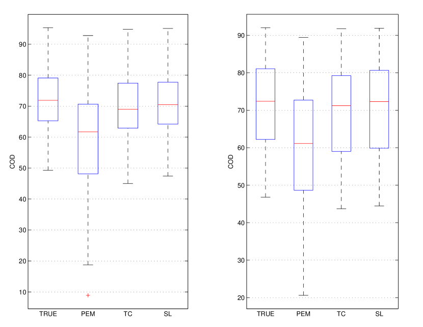
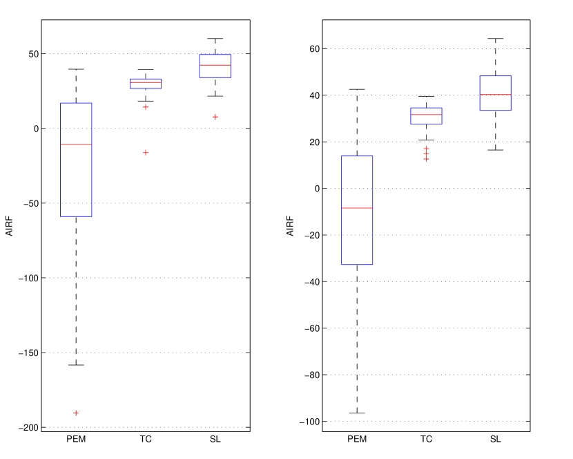
shows the COD in the first two experiments. One can see that SL provides a slightly better performance than TC. On the other hand, SL provides better estimators for the predictor coefficients than the TC, Figure 3.

Figure 3: Average impulse response fit in the first experiment (left panel) and in the second experiment (right panel).

Finally, Figure 4

Figure 4: One step ahead coefficient of determination in the third experiment.

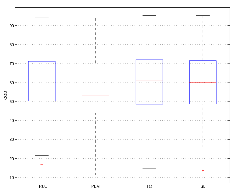
shows the COD in the third experiment. The median of SL is slightly worse than the one of TC. On the other hand, the bottom whisker of SL is better than the one of TC. Indeed, SL simplified the S+L network, see Table I, increasing the robustness of the estimated predictor impulse response coefficients.

VII Conclusions

In this paper, we proposed a Gaussian regression approach to identify multivariate stochastic processes having sparse network with few latent nodes. Simulations show that our approach is able to identify a S+L network which does not compromise the prediction performance.

References

- [1] A. Abdelwahab, O. Amor, and T. Abdelwahed. The analysis of the interdependence structure in international financial markets by graphical models. Int. Res. J. Finance Econ., 15:291–306, 2008.
- [2] A. Aravkin, J. Burke, A. Chiuso, and G. Pillonetto. Convex vs non-convex estimators for regression and sparse estimation: the mean squared error properties of ard and glasso. Journal of Machine Learning Research, 15:217–252, 2014.
- [3] N. Aronszajn. Theory of reproducing kernels. Trans. Amer. Math. Soc., 68:337–404, 1950.
- [4] S. Bonettini, A. Chiuso, and M. Prato. A scaled gradient projection method for Bayesian learning in dynamical systems. SIAM Journal on Scientific Computing, 37:1297–1318, 2015.
- [5] V. Chandrasekaran, P. Parrilo, and A. Willsky. Latent variable graphical model selection via convex optimization. Annals of Statistics (with discussion), 40(4):1935–2013, Apr. 2010.
- [6] T. Chen, H. Ohlsson, and L. Ljung. On the estimation of transfer functions, regularizations and gaussian processes-revisited. Automatica, 48(8):1525–1535, 2012.
- [7] A. Chiuso and G. Pillonetto. A Bayesian approach to sparse dynamic network identification. Automatica, 48(8):1553–1565, 2012.
- [8] M. Choi, V. Chandrasekaran, and A. Willsky. Gaussian multiresolution models: Exploiting sparse markov and covariance structure. IEEE Transactions on Signal Processing, 58(3):1012–1024, March 2010.
- [9] T. Cover and J. Thomas. Information Theory. Wiley, New York, 1991.
- [10] M. Deistler and C. Zinner. Modelling high-dimensional time series by generalized linear dynamic factor models: An introductory survey. Communications in Information & Systems, 7(2):153–166, 2007.
- [11] G. Goodwin, M. Gevers, and B. Ninness. Quantifying the error in estimated transfer functions with application to model order selection. IEEE Transactions on Automatic Control, 37(7):913–928, Jul 1992.
- [12] C. Granger. Investigating causal relations by econometric models and cross-spectral methods. Econometrica, 37(3):424–438, Aug. 1969.
- [13] E Kolaczyk. Statistical analysis of network data: methods and models. Springer, 2009.
- [14] S. Lauritzen. Graphical Models. Oxford University Press, Oxford, 1996.
- [15] L. Ljung. System Identification (2Nd Ed.): Theory for the User. Prentice Hall, New Jersey, 1999.
- [16] G. Pillonetto, A. Chiuso, and G. De Nicolao. Prediction error identification of linear systems: A nonparametric gaussian regression approach. Automatica, 47(2):291–305, 2011.
- [17] G. Pillonetto and G. De Nicolao. A new kernel-based approach for linear system identification. Automatica, 46:81–93, 2010.
- [18] G. Pillonetto, F. Dinuzzo, T. Chen, G. De Nicolao, and L. Ljung. Kernel methods in system identification, machine learning and function estimation: A survey. Automatica, 50(3):657–682, 2014.
- [19] T. Söderström and P. Stoica, editors. System Identification. Prentice Hall, New Jersey, 1988.
- [20] A. Werhli, M. Grzegorczyk, and D. Husmeier. Comparative evaluation of reverse engineering gene regulatory networks with relevance networks, graphical gaussian models and Bayesian networks. Bioinformatics, 22(20):2523–2531, 2006.
- [21] M. Zorzi and R. Sepulchre. AR identification of latent-variable graphical models. Conditionally accepted in IEEE Transactions on Automatic Control, 2015.