On the convergence of a Risk Sensitive like Filter

Abstract

In this paper, we analyze the convergence of a risk sensitive like filter where the risk sensitivity parameter is time varying. Such filter has a Kalman like structure and its gain matrix is updated according to a distorted version of the Riccati iteration. We show that the iteration converges to a fixed point by using the contraction analysis.

I Introduction

Physical systems are often modeled by (nominal) linear models. One reason is that the corresponding filtering problem is tractable, for instance if we consider the Gauss-Markov state space model then we obtain the Kalman filter. On the other hand, linear models are rather simple and thus introduce modeling errors. This implies that the optimal filter may not perform well in the realty.

One possible strategy to deal with such problem is to use robust filtering. The pioneering works are due by Kassam, Poor and their collaborators, [10],[14]. This paradigm can be sketched as follows. One player (say, nature) selects the least favorable model in an allowable neighborhood about the nominal model, while the other player designs the optimal filter based on that least favorable model. Therefore, the optimal filter is obtained by solving a minimax problem. However, the implementation of such a filter can be very difficult because it depends on the characterization of the allowable neighborhood. To overcome this difficulty, a new class of robust filters based on the minimization of risk sensitive functions, which penalize large estimation errors, was introduced in [15],[17],[2]. The sensitivity to large errors is tuned by a risk sensitivity parameter. This approach considers Gauss-Markov state space models and the resulting robust filter is a Kalman like filter where the gain matrix is updated according to a distorted version of the Riccati iteration (say, risk sensitive Riccati iteration). Unfortunately, this method only considers the nominal model. In [12], a new minimax robust state space filtering problem was examineted. In this approach, at each time step all possible increments of the state space model are described by a ball about the nominal increment. Its radius is fixed a priori and represents the tolerance budget available at each time step. Therefore, the nature selects the least favorable model increment in the allowable ball, and the other player designs the optimal filter based on that least favorable model. It turns out the resulting robust filter is a risk sensitive like filter where the risk sensitivity parameter is now time varying. Accordingly, the gain matrix updating is governed by a risk sensitive like Riccati iteration.

An important issue for Kalman like filters is their convergence. In [3], under the assumption that the Gauss-Markov state space model is reachable and observable, it has been established that the Riccati mapping is a contraction for the Riemann metric associated to the cone of positive definite matrices, and thus the Riccati iteration asymptotically converges. The same result can be proved by using the Thompson part metric [11, 5]. In [13], a similar contraction analysis has been considered to prove the convergence of the risk sensitive Riccati iteration. Here, the problem has been formulated in Krein space, see [6], [7]. Then, it has been shown that the $N$-block risk sensitive Riccati mapping is strictly contractive for the Riemann metric by choosing the risk sensitivity parameter sufficiently small. Regarding the risk sensitive like Riccati iteration, it seems to converge [12], but no convergence result has been proved yet.

In this paper, we consider a similar contraction analysis to prove that the risk sensitive like filter in [12] asymptotically converges for tolerance values sufficiently small. More precisely, we formulate the filtering problem in Krein space and then we show that the N-block risk sensitive like Riccati mapping is strictly contractive provided that the time varying risk sensitivity parameter is smaller than a constant parameter. Moreover, it is always possible to find a lower bound of this iteration after a finite number of steps. As we will see, both the constant parameter and the lower bound allow to characterize a range of values of the tolerance for which the iteration converges.

The paper is organized as follows. In Section II we review the risk sensitive like filter presented in [12]. In Section III we review the Thompson part metric and contractive mappings needed for the following contraction analysis. In Section IV we construct the $N$-block risk sensitive like Riccati mapping. In Section V we characterize a range of values of $c$ for which the mapping is a strict contraction. Finally, in Section VI we provide an example. Throughout the paper, $\cal P$ denotes the cone of positive definite symmetric matrices, and $\overline{\cal P}$ its closure. Given $P\in\cal P$, $\lambda_{1}(P)\geq\lambda_{2}(P)\geq\ldots\lambda_{n}(P)>0$ are its eigenvalues sorted in decreasing order.

II Risk sensitive like Filtering

Consider a discrete-time stochastic process $y_{t}$ described by a nominal Gauss-Markov state space model of the form

$$x_{t+1} = Ax_{t}+Bu_{t}$$ (1)

$$y_{t} = Cx_{t}+Dv_{t},\;\;t\geq 0$$ (2)

where the state $x_{t}\in\mathbb{R}^{n}$, the process noise $u_{t}\in\mathbb{R}^{m}$, and the observation noise $v_{t}\in\mathbb{R}^{p}$. The noises $u_{t}$ and $v_{t}$ are assumed to be zero-mean WGN processes with normalized covariance matrices and independent, that is

$$E\Big{[}\left[\begin{array}[]{c}u_{t}\\ v_{t}\\ \end{array}\right]\left[\begin{array}[]{cc}u_{s}&v_{s}\\ \end{array}\right]\Big{]}=\left[\begin{array}[]{cc}I_{m}&0\\ 0&I_{p}\\ \end{array}\right]\delta_{t-s}\>,$$

where $\delta_{t}$ denotes the Kronecker delta function. The initial state vector $x_{0}$ is assumed independent of the noises $u_{t}$ and $v_{t}$ with nominal probability density

$$p_{0}(x_{0})\sim{\cal N}(0,P_{0}).$$

The pairs $(A,B)$ and $(A,C)$ are assumed to be reachable and observable, respectively. Moreover, we assume that the noises $u_{t}$ and $v_{t}$ affect all the components of the dynamics (1) and observations (2), that is $BB^{T}$ and $DD^{T}$ are positive definite. As observed in [12], this is a natural property to demand when the relative entropy is used to measure the proximity of statistical models, see below.

The robust filter proposed in [12] is designed according to the minimax point of view. More precisely, at time $t$, the nature selects the least favorable increment of the state space model in a ball about the nominal increment given by (1)-(2). Such a ball is characterized by requiring that the Kullback-Leibler divergence, [4], between the two model increments is smaller than or equal to the tolerance $c\geq 0$. Note that, $c$ is fixed by the user. More precisely, the larger $c$ is, the worse increments the nature can select.

It turns out that the robust estimator $\hat{x}_{t+1}$ of $x_{t+1}$, given the observations $y_{t},y_{t-1},\ldots,y_{0}$, obeys the Kalman like recursion

$$\hat{x}_{t+1}=A\hat{x}_{t}+K_{t}\nu_{t}\>,$$ (3)

where

$$\nu_{t}\stackrel{{\scriptstyle\triangle}}{{=}}y_{t}-C\hat{x}_{t}$$ (4)

is the innovations process. In (3), the gain matrix

$$K_{t}=A(P_{t}^{-1}-\theta_{t-1}I_{n})^{-1}C^{T}(R_{t}^{\nu})^{-1}\>,$$ (5)

where

$$R_{t}^{\nu}=E[\nu_{t}\nu_{t}^{T}]=C(P_{t}^{-1}-\theta_{t-1}I_{n})^{-1}C^{T}+DD^{T}$$ (6)

represents the variance of the innovations process, $\theta_{t-1}$ with

$$0<\theta_{t-1}<(\lambda_{1}(P_{t}))^{-1}$$ (7)

is the unique solution to the equation

$$\gamma(\theta_{t-1},P_{t})=c$$ (8)

where

$$\gamma(\theta,P)\triangleq\frac{1}{2}\left[\log\det(I-\theta P)+\mathrm{tr}[(I-\theta P)^{-1}]-n\right],$$ (9)

and if $\tilde{x}_{t}=x_{t}-\hat{x}_{t}$ denotes the state prediction error, its variance matrix $P_{t}=E[\tilde{x}_{t}\tilde{x}_{t}^{T}]$ obeys the distorted Riccati iteration

$$P_{t+1}=r^{R}_{c}(P_{t})$$ (10)

with initial condition $P_{0}$. The mapping $r^{R}_{c}(\cdot)$ is defined by

$$r^{R}_{c}(P_{t})\stackrel{{\scriptstyle\triangle}}{{=}}A[P_{t}^{-1}+C^{T}(DD^{T})^{-1}C-\theta_{t-1}I]^{-1}A^{T}+BB^{T}.$$

Note that, the robust filter (3)-(8) is a risk sensitive like filter, [17], [16, Chapter 10]. In the classic formulation, however, the risk sensitive Riccati mapping is defined as

$$r^{RS}_{\theta}(P)\stackrel{{\scriptstyle\triangle}}{{=}}A[P^{-1}+C^{T}(DD^{T})^{-1}C-\theta I]^{-1}A^{T}+BB^{T}$$

where the risk sensitivity parameter $\theta\geq 0$ is constant and does not depend on $P$. Moreover, for $\theta=0$ (risk neutral case) we obtain the Riccati mapping

$$r(P)\stackrel{{\scriptstyle\triangle}}{{=}}A[P^{-1}+C^{T}(DD^{T})^{-1}C]^{-1}A^{T}+BB^{T}.$$

Finally, it is worth noting that (7) implies that $r^{R}_{c}(P)\in{\cal P}$ for each $P\in{\cal P}$, that is $r_{c}^{R}(\cdot)$ is a mapping of ${\cal P}$. Such a property does not hold for the classic risk sensitive mapping because it may occur that $r^{RS}_{\theta}(P)\notin{\cal P}$ even when $P\in{\cal P}$, [13].

III Thompson part metric and contraction mappings

If $P$ is an element of ${\cal P}$ with eigendecomposition

$$P=U\Lambda U^{T}$$ (11)

where $U$ is an orthogonal matrix formed by normalized eigenvectors of $P$ and $\Lambda=\mbox{diag}\,\{\lambda_{1},\ldots,\lambda_{n}\}$ is the diagonal eigenvalue matrix of $P$, the square-root of $P$ is defined as

$$P^{1/2}=U\Lambda^{1/2}U^{T}$$

where $\Lambda^{1/2}$ is diagonal, with entries $\lambda_{i}^{1/2}$ for $1\leq i\leq n$. Similarly, the logarithm of $P$ is the matrix specified by

$$\log(P)=U\log(\Lambda)U^{T}\>,$$

where $\log(\Lambda)$ is diagonal with entries $\log(\lambda_{i})$ for $1\leq i\leq n$. Let $P$ and $Q$ be two positive definite matrices of ${\cal P}$. Then $P^{-1}Q$ is similar to $P^{-1/2}QP^{-1/2}$, so they have the same eigenvalues, and $P^{-1/2}QP^{-1/2}$ is positive definite. The Thompson part metric between $P$ and $Q$ is defined as

$$d_{T}(P,Q) = ||\log(P^{-1/2}QP^{-1/2})||_{2}$$

$$= \max\{\log(\lambda_{1}(P^{-1}Q)),\log(\lambda_{1}(Q^{-1}P))\}\>,$$

where $||\cdot||_{2}$ denotes the spectral norm.

Let $f(\cdot)$ be a non expansive mapping of $\mathcal{P}$. Its contraction coefficient (or Lipschitz constant) is defined as

$$\xi(f)=\sup_{P,Q\in{\cal P},P\neq Q}\frac{d_{T}(f(P),f(Q))}{d_{T}(P,Q)}\>.$$ (12)

From (12) we get

$$d_{T}(f(P),f(Q))\leq\xi(f)d_{T}(P,Q).$$

Moreover, if $\xi(f)<1$, then $f$ is a strictly contractive mapping.

If $f$ is a strict contraction of ${\cal P}$ for the metric $d_{T}$, by the Banach fixed point theorem [1, p. 244], there exists a unique fixed point $P$ of $f$ in $\bar{\cal P}$ satisfying $P=f(P)$. Moreover, if the $N$-fold composition $f^{N}$ of a non-expansive mapping $f$ (or simply $N$-block mapping of $f$) is strictly contractive, then $f$ has a unique fixed point. Furthermore this fixed point can be evaluated by performing the iteration $P_{k+1}=f(P_{k})$ starting from any initial point $P_{0}$ of ${\cal P}$. We will consider in particular the Riccati like mapping defined by

$$f(P)=M[P^{-1}+\Omega]^{-1}M^{T}+W$$ (13)

where $P$, $\Omega$ and $W$ are symmetric real positive definite matrices and $M$ is a square real, but not necessarily invertible, matrix. For this mapping the following result was established in [11, Th. 5.3].

Lemma III.1

The mapping in (13) is strictly contractive with

$$\xi(f)\leq\left(\frac{\sqrt{\lambda_{1}(\Omega^{-1}M^{T}W^{-1}M)}}{1+\sqrt{1+\lambda_{1}(\Omega^{-1}M^{T}W^{-1}M)}}\right)^{2}.\>$$ (14)

Lemma III.1 is the key result we will use to prove that iteration (10) converges for any $P_{0}\in\cal P$, and thus the risk sensitive like filter converges.

IV $N$-block risk sensitive like Riccati mapping

The robust filter (3)-(8) can be interpreted as solving a standard least-square filtering problem with time-varying parameters in Krein space. The Krein state space model consists of dynamics (1) and observations (2), to which we must adjoin the new observations

$$0=x_{t}+v_{t}^{R}\>.$$ (15)

The components of noise vectors $u_{t}$, $v_{t}$ and $v_{t}^{R}$ now belong to a Krein space and have the inner product

$$\left\langle\left[\begin{array}[]{c}u_{t}\\ v_{t}\\ v_{t}^{R}\end{array}\right]\,,\,\left[\begin{array}[]{c}u_{s}\\ v_{s}\\ v_{s}^{R}\end{array}\right]\right\rangle=\left[\begin{array}[]{ccc}I_{m}&0&0\\ 0&I_{p}&0\\ 0&0&-(\theta_{t-1})^{-1}I_{n}\\ \end{array}\right]\delta_{t-s}.$$ (16)

Note that, in the classical risk sensitive framework, [6, 7], $v_{t}^{R}$ with $t\geq 0$ are identically distributed, whereas are not in this setting. Since $x_{t}$ is Gauss-Markov, the downsampled process $x_{k}^{d}=x_{kN}$, with $N$ integer, is also Gauss-Markov with state space model

$$x_{k+1}^{d} = A^{N}x_{k}^{d}+{\cal R}_{N}{\bf u}_{k}^{N}$$ (17)

$${\bf y}_{k}^{N} = {\cal O}_{N}x_{k}^{d}+{\cal D}_{N}{\bf v}_{k}^{N}+{\cal H}_{N}{\bf u}_{k}^{N}$$ (18)

$${\bf 0} = {\cal O}_{N}^{R}x_{k}^{d}+{\bf v}_{k}^{RN}+{\cal L}_{N}{\bf u}_{k}^{N}\>$$ (19)

where

$${\bf u}_{k}^{N} \triangleq \left[\begin{array}[]{cccc}u_{kN+N-1}^{T}&u_{kN+N-2}^{T}&\ldots&u_{kN}^{T}\end{array}\right]^{T}$$ (21)

$${\bf v}_{k}^{N} \triangleq \left[\begin{array}[]{cccc}v_{kN+N-1}^{T}&v_{kN+N-2}^{T}&\ldots&v_{kN}^{T}\end{array}\right]^{T}$$ (23)

$${\bf y}_{k}^{N} \triangleq \left[\begin{array}[]{cccc}y_{kN+N-1}^{T}&y_{kN+N-2}^{T}&\ldots&y_{kN}^{T}\end{array}\right]^{T}$$ (25)

$${\bf v}_{k}^{RN} \triangleq \left[\begin{array}[]{ccc}(v_{kN+N-1}^{R})^{T}&(v_{kN+N-2}^{R})^{T}&\ldots\end{array}\right.$$ (29)

$$\hskip 99.58464pt\left.\begin{array}[]{cc}\ldots&(v_{kN}^{R})^{T}\end{array}\right]^{T}.$$

In the model (17)–(19)

$${\cal R}_{N} \triangleq \left[\begin{array}[]{cccc}B&AB&\ldots&A^{N-1}B\end{array}\right]$$ (31)

$${\cal O}_{N} \triangleq \left[\begin{array}[]{cccc}(CA^{N-1})^{T}&\ldots&(CA)^{T}&C^{T}\end{array}\right]^{T}$$ (33)

$${\cal O}_{N}^{R} \triangleq \left[\begin{array}[]{cccc}(A^{N-1})^{T}&\ldots&(A)^{T}&I\end{array}\right]^{T}$$ (35)

$${\cal D}_{N} \triangleq I_{N}\otimes D.$$ (36)

Note that ${\cal R}_{N}$ and ${\cal O}_{N}$ denote respectively the $N$-block reachability and observability matrices of system (1)–(2), where the blocks forming ${\cal O}_{N}$ are written from bottom to top instead of the usual top to bottom convention. If the pairs $(A,B)$ and $(C,A)$ are reachable and observable, ${\cal R}_{N}$ and ${\cal O}_{N}^{T}$ have full row rank for $N\geq n$. In (18) and (19), if

$$H_{t} \triangleq \left\{\begin{array}[]{cc}CA^{t-1}B&t\geq 1\\ 0&\mbox{otherwise }\end{array}\right.$$ (39)

$$L_{t} \triangleq \left\{\begin{array}[]{cc}A^{t-1}B&t\geq 1\\ 0&\mbox{otherwise}\end{array}\right.$$ (42)

${\cal H}_{N}$ and ${\cal L}_{N}$ are block Hankel matrices defined as follows

$${\cal H}_{N} \triangleq \left[\begin{array}[]{cccccc}0&H_{1}&H_{2}&\cdots&H_{N-2}&H_{N-1}\\ 0&0&H_{1}&H_{2}&\cdots&H_{N-2}\\ 0&0&0&H_{1}&\cdots&H_{N-3}\\ \vdots&\vdots&\vdots&&\vdots&\vdots\\ 0&0&\cdots&\cdots&0&H_{1}\\ 0&0&\cdots&\cdots&\cdots&0\end{array}\right]$$ (49)

$${\cal L}_{N} \triangleq \left[\begin{array}[]{cccccc}0&L_{1}&L_{2}&\cdots&L_{N-2}&L_{N-1}\\ 0&0&L_{1}&L_{2}&\cdots&L_{N-2}\\ 0&0&0&L_{1}&\cdots&L_{N-3}\\ \vdots&\vdots&\vdots&&\vdots&\vdots\\ 0&0&0&\cdots&\cdots&L_{1}\\ 0&0&0&\cdots&\cdots&0\\ \end{array}\right].$$ (56)

The Krein space inner product of the observation noise vector

$$\left[\begin{array}[]{c}{\bf w}_{k}^{N}\\ {\bf w}_{k}^{RN}\end{array}\right]=\left[\begin{array}[]{c}{\cal D}_{N}{\bf v}_{k}^{N}\\ {\bf v}_{k}^{RN}\end{array}\right]+\left[\begin{array}[]{c}{\cal H}_{N}\\ {\cal L}_{N}\end{array}\right]{\bf u}_{k}^{N}$$

admits the following decomposition

$${\cal K}_{\Theta_{N,k}}\stackrel{{\scriptstyle\triangle}}{{=}}\left\langle\left[\begin{array}[]{c}{\bf w}_{k}^{N}\\ {\bf w}_{k}^{RN}\end{array}\right]\,,\,\left[\begin{array}[]{c}{\bf w}_{k}^{N}\\ {\bf w}_{k}^{RN}\end{array}\right]\right\rangle$$ (61)

$$= \left[\begin{array}[]{cc}{\cal D}_{N}{\cal D}_{N}^{T}&0\\ 0&-(\Theta_{N,k})^{-1}\end{array}\right]+\left[\begin{array}[]{c}{\cal H}_{N}\\ {\cal L}_{N}\end{array}\right]\left[\begin{array}[]{cc}{\cal H}_{N}^{T}&{\cal L}_{N}^{T}\end{array}\right]$$ (67)

$$= \left[\begin{array}[]{cc}I_{Np}&0\\ {\cal L}_{N}{\cal H}_{N}^{T}({\cal D}_{N}{\cal D}_{N}^{T}+{\cal H}_{N}{\cal H}_{N}^{T})^{-1}&I_{Nn}\end{array}\right]$$ (76)

$$\hskip 8.5359pt\times\left[\begin{array}[]{cc}{\cal D}_{N}{\cal D}_{N}^{T}+{\cal H}_{N}{\cal H}_{N}^{T}&0\\ 0&S_{\Theta_{N,k}}\end{array}\right]$$

$$\hskip 8.5359pt\times\left[\begin{array}[]{cc}I_{Np}&({\cal D}_{N}{\cal D}_{N}^{T}+{\cal H}_{N}{\cal H}_{N}^{T})^{-1}{\cal H}_{N}{\cal L}_{N}^{T}\\ 0&I_{Nn}\end{array}\right]\>,$$

where

$$S_{\Theta_{N,k}}\stackrel{{\scriptstyle\triangle}}{{=}}-(\Theta_{N,k})^{-1}+{\cal L}_{N}(I_{Nm}+{\cal H}_{N}^{T}({\cal D}_{N}{\cal D}_{N}^{T})^{-1}{\cal H}_{N})^{-1}{\cal L}_{N}^{T}$$ (77)

denotes the Schur complement of the $(1,1)$ block inside ${\cal K}_{\Theta_{N,k}}$ with

$$\Theta_{N,k}\stackrel{{\scriptstyle\triangle}}{{=}}\mathrm{diag}(\theta_{kN+N-2},\theta_{kN+N-3},\ldots,\theta_{kN-1})\otimes I_{n}.$$ (78)

The projection of noise vector ${\bf u}_{k}^{N}$ on the Krein subspace spanned by the observation noise vector $\left[\begin{array}[]{cc}({\bf w}_{k}^{N})^{T}&({\bf w}_{k}^{RN})^{T}\end{array}\right]^{T}$ is then given by

$$\hat{\bf u}_{k}^{N}=\left[\begin{array}[]{cc}G_{k}&G_{k}^{R}\end{array}\right]\left[\begin{array}[]{c}{\bf w}_{k}^{N}\\ {\bf w}_{k}^{NR}\end{array}\right]\>,$$

where

$$\left[\begin{array}[]{cc}G_{k}&G_{k}^{R}\end{array}\right]=\left[\begin{array}[]{cc}{\cal H}_{N}^{T}&{\cal L}_{N}^{T}\end{array}\right]({\cal K}_{\Theta_{N,k}})^{-1}\>,$$

and the residual $\tilde{\bf u}_{k}^{N}={\bf u}_{k}^{N}-\hat{\bf u}_{k}^{N}$ has for inner product

$${\cal Q}_{\Theta_{N,k}}\stackrel{{\scriptstyle\triangle}}{{=}}\langle\tilde{\bf u}_{k}^{N}\,,\,\tilde{\bf u}_{k}^{N}\rangle$$

$$\hskip 8.5359pt=I_{Nm}-\left[\begin{array}[]{cc}G_{k}&G_{k}^{R}\end{array}\right]{\cal K}_{\Theta_{N,k}}\left[\begin{array}[]{c}G_{k}^{T}\\ (G_{k}^{R})^{T}\end{array}\right]$$ (82)

$$\hskip 8.5359pt=[I_{Nm}+{\cal H}_{N}^{T}({\cal D}_{N}{\cal D}_{N}^{T})^{-1}{\cal H}_{N}-{\cal L}_{N}^{T}\Theta_{N,k}{\cal L}_{N}]^{-1}\>.$$

Then by multiplying the observation equation obtained by combining equations (18) and (19) by ${\cal R}_{N}\left[\begin{array}[]{cc}G_{k}&G_{k}^{R}\end{array}\right]$ and subtracting it from (17), we obtain the state space equation

$$x_{k+1}^{d}=\alpha_{N,k}x_{k}^{d}+{\cal R}_{N}\tilde{\bf u}_{k}^{N}+{\cal R}_{N}G_{k}{\bf y}_{k}^{N}$$ (83)

with

$$\alpha_{N,k}\stackrel{{\scriptstyle\triangle}}{{=}}A^{N}-{\cal R}_{N}[G_{k}{\cal O}_{N}+G_{k}^{R}{\cal O}_{N}^{R}]\>,$$

where the driving noise $\tilde{\bf u}^{N}_{k}$is now orthogonal to the noises ${\bf w}_{k}^{N}$ and ${\bf w}_{k}^{RN}$ appearing in observation equations (18) and (19). Accordingly, the time-varying Riccati iteration associated to the downsampled model takes the form

$$P_{k+1}^{d}=r^{d}_{c}(P_{k}^{d})$$ (84)

where

$$r^{d}_{c}(P_{k}^{d})\stackrel{{\scriptstyle\triangle}}{{=}}\alpha_{N,k}[(P_{k}^{d})^{-1}+\Omega_{\Theta_{N,k}}]^{-1}\alpha_{N,k}^{T}+W_{\Theta_{N,k}}$$

$$\Omega_{\Theta_{N,k}} \triangleq \left[\begin{array}[]{cc}{\cal O}_{N}^{T}&({\cal O}_{N}^{R})^{T}\end{array}\right]{\cal K}_{\Theta_{N,k}}^{-1}\left[\begin{array}[]{c}{\cal O}_{N}\\ {\cal O}_{N}^{R}\end{array}\right]$$ (88)

$$= \Omega_{N}+{\cal J}_{N}^{T}S_{\Theta_{N,k}}^{-1}{\cal J}_{N}$$ (89)

with

$${\cal J}_{N} \stackrel{{\scriptstyle\triangle}}{{=}} {\cal O}_{N}^{R}-{\cal L}_{N}{\cal H}_{N}^{T}[{\cal D}_{N}{\cal D}_{N}^{T}+{\cal H}_{N}{\cal H}_{N}^{T}]^{-1}{\cal O}_{N}$$

$$\Omega_{N} \stackrel{{\scriptstyle\triangle}}{{=}} {\cal O}_{N}^{T}({\cal D}_{N}{\cal D}_{N}^{T}+{\cal H}_{N}{\cal H}_{N}^{T})^{-1}{\cal O}_{N}$$

and

$$W_{\Theta_{N,k}}\triangleq{\cal R}_{N}{\cal Q}_{\Theta_{N,k}}{\cal R}_{N}^{T}\>.$$ (90)

V Convergence of the risk sensitive like filter

In this Section we show that the filter (3)-(8) asymptotically converges, or equivalently iteration (10) converges for any $P_{0}\in\cal P$, for tolerance values sufficiently small.

The idea is to find an upper bound for $c$, say $c_{\mathrm{MAX}}$, for which the Gramians $\Omega_{\Theta_{N,k}}$ and $W_{\Theta_{N,k}}$ are positive definite for $k\geq\tilde{q}$ and $\tilde{q}$ is a fixed integer number. Then, by Lemma III.1, $r_{c}^{d}(\cdot)$ is a strict contraction for $k\geq\tilde{q}$. Since $r_{c}^{d}(\cdot)$ is the $N$-block mapping of $r_{c}^{R}(\cdot)$, we conclude that iteration (10) converges.

Note that, $\Omega_{\Theta_{N,k}}$ and $W_{\Theta_{N,k}}$ depend on the positive definite matrix $\Theta_{N,k}$. It is not difficult to see that, a sufficient condition to guarantee ${\cal Q}_{\Phi}$ positive definite for $0\preceq\Phi\prec\tilde{\phi}_{N}I_{Nn}$, and thus also $W_{\Phi}$ for $N\geq n$, is that

$$\tilde{\phi}_{N}=\frac{1}{\lambda_{1}({\cal L}_{N}(I_{Nm}+{\cal H}_{N}^{T}({\cal D}_{N}{\cal D}_{N}^{T})^{-1}{\cal H}_{N})^{-1}{\cal L}_{N}^{T})}>0.$$

Such a condition also guarantees that $S_{\Phi}^{-1}$ is negative definite.

Lemma V.1

Let $\Phi_{1}$ and $\Phi_{2}$ be such that $0\preceq\Phi_{2}\preceq\Phi_{1}\prec\tilde{\phi}_{N}I_{Nn}$. Then,

$$\Omega_{\Phi_{1}} \preceq \Omega_{\Phi_{2}}$$

$$W_{\Phi_{1}} \succeq W_{\Phi_{2}}.$$ (91)

Note that

$$\left.\Omega_{\Phi}\right|_{\Phi=0} = \Omega_{N}$$

$$\left.W_{\Phi}\right|_{\Phi=0} = {\cal R}_{N}(I_{Nm}+{\cal H}_{N}^{T}({\cal D}_{N}{\cal D}_{N}^{T})^{-1}{\cal H}_{N})^{-1}{\cal R}_{N}^{T}$$

which are positive definite matrices for $N\geq n$ because the pairs $(C,A)$ and $(A,B)$ are observable and reachable, respectively. Accordingly, in view of Lemma V.1, there exists a constant $\phi_{N}>0$ with $N\geq n$ such that

$$\Omega_{\Phi},W_{\Phi}\succ 0,\;\;\forall\,0\preceq\Phi\prec\phi_{N}I_{Nn}.$$ (92)

As noticed before, $W_{\Phi}$ is positive definite over the range $0\preceq\Phi\prec\tilde{\phi}_{n}I_{Nn}$. Then, we set $\phi_{N}=\tilde{\phi}_{N}$ and check whether $\Omega_{\phi_{N}I_{Nn}}$ is positive definite or not. If not, we decrease $\phi_{N}$ up to $\Omega_{\phi_{N}I_{Nn}}$ becomes positive semi-definite but singular. In this way, (92) holds. Therefore, if $\Theta_{N,k}\prec\phi_{N}I_{Nn}$ for $k\geq\tilde{q}$, then the Gramians $\Omega_{\Theta_{N,k}}$ and $W_{\Theta_{N,k}}$ are positive definite for $k\geq\tilde{q}$, and thus iteration (10) converges.

Now, we characterize an upper bound for $c$, say $c_{MAX}$, which guarantees that $\Theta_{N,k}\prec\phi_{N}I_{Nn}$ for $k\geq\tilde{q}$. To this aim, we need the following two Propositions.

Proposition V.1

Consider iterations (10) and (84) with an arbitrary $P_{0}\in{\cal P}$. Moreover, consider the iteration

$$\overline{P}_{t+1}=r(\overline{P}_{t}),\;\;\overline{P}_{0}=BB^{T}.$$

Then, after a finite number of steps, say $q+1$, we have

$$P_{t}\succeq\overline{P}_{q},\;\;t\geq q+1,$$

and after $\tilde{q}=\lceil\frac{q+1}{N}\rceil$ steps

$$P_{k}^{d}\succeq\overline{P}_{q},\;\;k\geq\tilde{q}.$$

Proposition V.2

Assuming that $0<\theta<(\lambda_{1}(P))^{-1}$, the following facts hold:

1. $\gamma(\cdot,P)$ is monotone increasing over $\mathbb{R}_{+}$

2. $\gamma(\theta,P)>0$ for any $P\in\bar{\cal P}$ with $P\neq 0$

3. If $P\succeq Q$ then $\gamma(\theta,P)\geq\gamma(\theta,Q)$

By Proposition V.1, $P_{t}\succeq\overline{P}_{q}$ with $t\geq q+1$ and $q$ is fixed. Then, by Proposition V.2, (8) implies that

$$\theta_{t-1}\leq\bar{\theta},\;\ \forall t\geq q+1$$

where $\bar{\theta}$ is such that $\gamma(\theta_{t-1},P_{t})=\gamma(\bar{\theta},\overline{P}_{q})$. Thus, condition $\Theta_{N,k}<\phi_{N}I_{Nn}$ for $k\geq\tilde{q}$ is guaranteed if we choose $c$ in such a way that $\bar{\theta}<\phi_{N}$. The idea is formalized in the following Proposition.

Proposition V.3

Let $c$ be such that $0<c<c_{MAX}$ with $c_{MAX}\triangleq\gamma(\phi_{N},\overline{P}_{q})$, $N\geq n$, and $q$ fixed. Then, the mapping $r^{d}_{c}(\cdot)$ is strictly contractive after $\lceil\frac{q+1}{N}\rceil$ steps. Accordingly, iteration (10) converges to a unique solution for any initial condition $P_{0}\in{\cal P}$.

Note that, by Proposition V.2, the map

$$q\mapsto\gamma(\phi_{N},\overline{P}_{q})$$

is nondecreasing. Thus, we have to choose $q$ sufficiently large in order to find a bigger $c_{MAX}$.

VI An Example

We consider the Gauss-Markov state space model earlier employed in [13]

$$A=\left[\begin{array}[]{cc}0.1&1\\ 0&1.2\\ \end{array}\right], B=I_{2}$$ (95)

$$C=\left[\begin{array}[]{cc}1&-1\\ \end{array}\right], D=1$$ (97)

with $n=2$, $m=2$ and $p=1$. We select $N=8$, in this way $N\geq n$. Note that, larger values of $N$ can be considered. We find that $\tilde{\phi}_{N}=1.6\cdot 10^{-2}$. In Figure 1

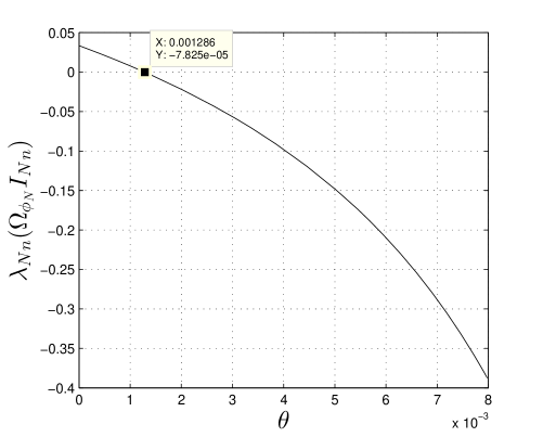
Figure 1: Minimum eigenvalue of $\Omega_{\phi_{N}I_{Nn}}$ over $\phi_{N}\in[0,8\cdot 10^{-3}]$.

we depict the smallest eigenvalue of $\Omega_{\phi_{N}I_{Nn}}$ over the range $\phi_{N}\in[0,8\cdot 10^{-3}]$. We find it becomes zero for $\phi_{N}\cong 1.3\times 10^{-3}$.

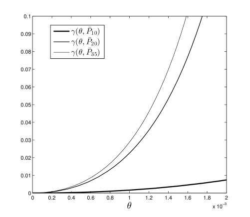
Figure 2: $\gamma(\theta,\bar{P}_{q})$ with $q=10$, $q=20$ and $q=35$.

In Figure 2 we depict $\gamma(\theta,\bar{P}_{10})$, $\gamma(\theta,\bar{P}_{20})$ and $\gamma(\theta,\bar{P}_{35})$. Note that, $\gamma(\phi_{N},\overline{P}_{10})\cong 2.9\cdot 10^{-3}$, $\gamma(\phi_{N},\overline{P}_{20})\cong 4.39\cdot 10^{-2}$ and $\gamma(\phi_{N},\overline{P}_{35})\cong 5.43\cdot 10^{-2}$. As expected, it is better to choose $\bar{P}_{35}$ for which we have $c_{\mathrm{MAX}}\cong 5.43\cdot 10^{-2}$. We conclude that the risk sensitive like filter (3)-(8) having tolerance parameter $c<5.43\cdot 10^{-2}$ and nominal model (95) asymptotically converges to a unique solution.

VII Conclusion

We analyzed the convergence of a risk sensitive like filter subject to an incremental tolerance. By contraction analysis, we showed that the corresponding $N$-block risk sensitive like Riccati mapping is strictly contractive for tolerance values sufficiently small. Accordingly, the corresponding iteration converges to a fixed point, and thus the robust filter converges.

A Proof of Lemma V.1

Let $\Phi$ and $\Delta$ belong to $\cal P$ and $\overline{{\cal P}}$, respectively, and such that $0\preceq\Phi+\Delta\prec\tilde{\phi}_{n}I_{Nn}$. The first variation of $S_{\Phi}^{-1}$ and ${\cal Q}_{\Phi}$ with respect to $\Phi$ in direction $\Delta$ are, respectively,

$$\delta S_{\Phi;\Delta}^{-1}=-(S_{\Phi})^{-1}\Phi^{-1}\Delta\Phi^{-1}S_{\Phi}^{-1}\preceq 0$$

and

$$\delta{\cal Q}_{\Phi;\Delta}={\cal Q}_{\Phi}{\cal L}_{N}^{T}\Delta{\cal L}_{N}{\cal Q}_{\Phi}\succeq 0\>.$$

This implies that

$$S^{-1}_{\Phi_{1}} \preceq S^{-1}_{\Phi_{2}}$$

$${\cal Q}_{\Phi_{1}} \succeq {\cal Q}_{\Phi_{2}}$$

with $0\preceq\Phi_{2}\preceq\Phi_{1}\preceq\tilde{\phi}_{N}I_{Nn}$. Accordingly,

$$\Omega_{\Phi_{1}} = \Omega_{N}+{\cal J}_{N}^{T}S^{-1}_{\Phi_{1}}{\cal J}_{N}\preceq\Omega_{N}+{\cal J}_{N}^{T}S^{-1}_{\Phi_{2}}{\cal J}_{N}=\Omega_{\Phi_{2}}$$

$$W_{\Phi_{1}} = {\cal R}_{N}{\cal Q}_{\Phi_{1}}{\cal R}_{N}^{T}\succeq{\cal R}_{N}{\cal Q}_{\Phi_{2}}{\cal R}_{N}^{T}=W_{\Phi_{2}}.$$

 

B Proof of Proposition V.1

Before proving the statement, we need the following two Lemmas. The first one regards a risk sensitive mapping property, [8, page 379].

Lemma .1

Let $P\in{\cal P}$ such that $P^{-1}-\theta_{1}I\in{\cal P}$ and $\theta_{1}\geq\theta_{2}\geq 0$. Then,

$$r_{\theta_{1}}^{RS}(P)\succeq r_{\theta_{2}}^{RS}(P).$$

Lemma .2

Consider the sequence

$$\tilde{P}_{t+1}=r^{R}_{c}(\tilde{P}_{t}),\;\;\tilde{P}_{0}\succeq BB^{T}.$$

Then,

$$\tilde{P}_{t}\succeq\overline{P}_{q},\;\;\forall\;t\geq q.$$ (98)

Proof:

We prove by induction that

$$\tilde{P}_{t}\succeq\overline{P}_{t},\;\;\forall\;t\geq 0.$$ (99)

Since, the sequence $\{\overline{P}_{t}\}$ is nondecreasing, see for instance [9], then the statement follows for a fixed value of $q$. For $t=0$, we have $\tilde{P}_{0}\succeq\overline{P}_{0}$. Assume that (99) holds at time $t$, then

$$\tilde{P}_{t+1}=r_{c}^{R}(\tilde{P}_{t})=r_{\theta_{t-1}}^{RS}(\tilde{P}_{t})\succeq r(\tilde{P}_{t})\succeq r(\overline{P}_{t})=\overline{P}_{t+1}$$ (100)

accordingly (99) also holds at time $t+1$.  

Now, we proceed with the proof of Proposition V.1. Consider the sequence generated by (10) with an arbitrary initial condition $P_{0}\in{\cal P}$. Note that $r_{c}^{R}(P)\succeq BB^{T}$ for any $P\in{\cal P}$. Accordingly $P_{t}\succeq BB^{T}$ for $t\geq 1$. We define the sequence $\{\tilde{P}_{t}\}$ with $\tilde{P}_{t}=P_{t+1}$ and $\tilde{P}_{0}=P_{1}\succeq BB^{T}$. In view of Lemma .2, we have that $\tilde{P}_{t}\succeq\overline{P}_{q}$ after $q$ steps. This implies $P_{t}\succeq\overline{P}_{q}$ for $t\geq q+1$. Noting that $P_{k}^{d}=P_{kN}$, the last statement follows.  

C Proof of Proposition V.2

The first point has been proved in [12]. Regarding the second point, $\gamma(\theta,P)$ is equal to the information divergence among the positive definite matrices $(I-\theta P)$ and $I$. Since $I-\theta P\neq I$, we get $\gamma(\theta,P)>0$. In order to prove the last point, we compute the first variation of $\gamma(\theta,P)$ with respect to $P$ in direction $Q\in\bar{\cal P}$:

$$\delta\gamma(\theta,P;Q)$$

$$=\hskip 5.69046pt\frac{\theta}{2}\mathrm{tr}[-(I-\theta P)^{-1}Q+(I-\theta P)^{-1}Q(I-\theta P)^{-1}]$$

$$\hskip 5.69046pt=\frac{\theta}{2}\mathrm{tr}[Q^{\frac{1}{2}}(I-\theta P)^{-\frac{1}{2}}(-I+(I-\theta P)^{-1})$$

$$\hskip 14.22636pt\times(I-\theta P)^{-\frac{1}{2}}Q^{\frac{1}{2}}]\succeq 0$$

where we exploited the fact that $(I-\theta P)^{-\frac{1}{2}}$ and $-I+(I-\theta P)^{-1}$ commute.  

D Proof of Proposition V.3

Consider iterations (10) and (84). As showed in Proposition V.1, after a finite number of steps, that is $q+1$ and $\tilde{q}=\lceil\frac{q+1}{N}\rceil$, we have, respectively,

$$P_{t}\succeq\overline{P}_{q},\;\;t\geq q+1$$

$$P^{d}_{k}\succeq\overline{P}_{q},\;\;k\geq\tilde{q}.$$

Since $c<\gamma(\phi_{N},\overline{P}_{q})$, by Proposition V.2 we have $\theta_{t}<\phi_{N}$ for $t\geq q+1$ and therefore $\Theta_{N,k}\prec\phi_{N}I_{Nn}$ for $k\geq\tilde{q}$. Accordingly, the Gramians, $\Omega_{\Theta_{N,k}}$ and $W_{\Theta_{N,k}}$ are positive definite for $k\geq\tilde{q}$. By Lemma III.1, the mapping $r^{d}_{c}(\cdot)$ is strictly contractive after $\tilde{q}$ steps. Since $r^{d}_{c}(\cdot)$ is the $N$-block mapping of $r_{c}^{R}(\cdot)$, it follows that the sequence generated by (10) converges for any $P_{0}\in{\cal P}$.

References

[1]
J. P. Aubin and I. Ekeland.
Applied Nonlinear Analysis.
Wiley, New York, 1984.
[2]
R. N. Banavar and J. L. Speyer.
Properties of risk-sensitive filters/estimators.
IEE Proc.-Control Theory Appl., 145, January 1998.
[3]
P. Bougerol.
Kalman filtering with random coefficients and contractions.
SIAM J. Control and Optimiz., 31:942–959, July 1993.
[4]
T. Cover and J. Thomas.
Information Theory.
Wiley, New York, 1991.
[5]
S. Gaubert and Z. Qu.
The contraction rate in Thompson’s part metric of order-preserving
flows on a cone–application to generalized Riccati equations.
Journal of Differential Equations, 256(8):2902–2948, 2014.
[6]
B. Hassibi, A. H. Sayed, and T. Kailath.
Linear estimation in Krein spaces. I. Theory.
IEEE Trans. Automat. Control, 41:18–33, January 1996.
[7]
B. Hassibi, A. H. Sayed, and T. Kailath.
Linear estimation in Krein spaces. II. Applications.
IEEE Trans. Automat. Control, 41:34–49, January 1996.
[8]
B. Hassibi, A. H. Sayed, and T. Kailath.
Indefinite-Quadratic Estimation and Control– A Unified Approach
to and Theories.
Soc. Indust. Appl. Math., Philadelphia, 1999.
[9]
T. Kailath, A. H. Sayed, and B. Hassibi.
Linear Estimation.
Prentice Hall, Upper Saddle River, NJ, 2000.
[10]
T. Kassam, S. amd Lim.
Robust Wiener filters.
J. Franklin Inst., 304:171–185, 1977.
[11]
H. Lee and Y. Lim.
Invariant metrics, contractions and nonlinear matrix equations.
Nonlinearity, 2:857–878, 2008.
[12]
B. C. Levy and R. Nikoukhah.
Robust state-space filtering under incremental model perturbations
subject to a relative entropy tolerance.
IEEE Trans. Automat. Control, 58:682–695, March 2013.
[13]
B. C. Levy and M. Zorzi.
A contraction analisys of the convergence of risk-sensitive filters.
Submitted, 2013.
[14]
H. Poor.
On robust Wiener filtering.
IEEE Trans. Automat. Control, 25(3):531–536, Jun 1980.
[15]
J. L. Speyer, J. Deyst, and D. H. Jacobson.
Optimization of stochastic linear systems with additive measurement
and process noise using exponential performance criteria.
IEEE Trans. Automat. Control, 19:358–366, 1974.
[16]
J.L. Speyer and W.H. Chung.
Stochastic Processes, Estimation, and Control.
Advances in Design and Control. Soc. Indust. Applied Math.,
Philadelphia, 2008.
[17]
P. Whittle.
Risk-sensitive Optimal Control.
J. Wiley, Chichester, England, 1980.