Full statistics of energy conservation in two times measurement protocols

Abstract

The first law of thermodynamics states that the average total energy current between different reservoirs vanishes at large times. In this note we examine this fact at the level of the full statistics of two times measurement protocols also known as the Full Counting Statistics. Under very general conditions, we establish a tight form of the first law asserting that the fluctuations of the total energy current computed from the energy variation distribution are exponentially suppressed in the large time limit. We illustrate this general result using two examples: the Anderson impurity model and a 2D spin lattice model.

Recent technical advances in the control of nanoscale systems have enabled the experimental study of out of equilibrium thermodynamics in the quantum regime Pekola (2015); Bustamante et al. (2005); Dubi and Di Ventra (2011); Ciliberto et al. (2013); Jezouin et al. (2013); Bérut et al. (2012); Toyabe et al. (2010); Koski et al. (2013); Küng et al. (2012). These new experiments allow for the assessment of fluctuations in addition to the mean heat and particle currents, thus leading to a renewed theoretical investigation of the related quantum thermodynamic laws.

One of the basic questions in this context concerns the energy flow between two initially isolated large systems $A$ and $B$. The purpose of this note is to study some consequences of energy conservation on the statistical properties of this flow.

By the first law, the average work performed by the interaction coupling the two systems is equal to the average heating of the combined system:

$$\Delta W_{t}=\Delta Q_{t}=\Delta Q_{t}^{A}+\Delta Q_{t}^{B}.$$

In the case of a sudden switching on/off of the interaction $V$, the average heating is given by

$$\Delta Q_{t}=-\langle V\rangle_{t}+\langle V\rangle_{0}$$ (1)

where $\langle\,\cdot\,\rangle_{t}$ denotes the expectation with respect to a suitable system state at time $t$. Whenever $V$ is bounded, (1) gives

$$\lim_{t\rightarrow\infty}\frac{\Delta Q_{t}}{t}=0.$$ (2)

The individual energy currents $\Delta Q_{t}^{A/B}/{t}$ are also expected to reach steady values $J^{A/B}$. They satisfy $J^{A}=-J^{B}$, and are non-vanishing for systems out of equilibrium.

This note concerns the statistical character of the first law related to the thermodynamics of open quantum systems at the mesoscopic scale. Our main result is a refinement of relation (2). It states that the fluctuations of the total energy current are exponentially suppressed in the large time limit.

The nature of work in quantum physics is more subtle than in classical physics Talkner et al. (2007). In the 1990’s Lesovik and Levitov introduced the concept of the Full Counting Statistics (FCS) in the study of charge transport Levitov and Lesovik (1993). The use of the FCS in the definition of work in quantum physics appeared in the early 2000’s in the works of J. Kurchan and H. Tasaki on the extension of the fluctuation relations to quantum systems Kurchan (2000); Tasaki (2000). The emerging idea is that in quantum mechanics work should not be understood as an observable. Instead, the work performed during a given time period is identified with the energy variation $\Delta E$ observed in a repeated measurement protocol where the system energy is measured at the beginning and at the end of the period. The distribution of the measured energy variation, $\mathbb{P}_{t}(\Delta E)$, is the work FCS (we comment on terminology in footnote ). This change of perspective opened a whole new area of research Esposito et al. (2009); Campisi et al. (2011). In particular, it allowed for the extension of the fluctuation relations to quantum systems Jarzynski and Wójcik (2004); Kurchan (2000); Esposito et al. (2009); Campisi et al. (2011); Jakšić et al. (2012); Tasaki (2000).

The fluctuation relations are intimately related to the second law of thermodynamics and have been extensively studied Kurchan (2000); Tasaki (2000); Esposito et al. (2009); Campisi et al. (2011); Crooks (2008); Jarzynski and Wójcik (2004); Evans and Searles (1994); Jakšić et al. (2012). Regarding the first law, the well known identity

$${\mathbb{E}}_{t}(\Delta E)=\Delta Q_{t}$$

and (2) give

$$\lim_{t\rightarrow\infty}{\mathbb{E}}_{t}\left(\frac{\Delta E}{t}\right)=0$$ (3)

where ${\mathbb{E}}_{t}$ denotes the expectation with respect to the FCS distribution ${\mathbb{P}}_{t}$ Talkner et al. (2007); Jakšić et al. (2012). In this note we sharpen (3) by showing that, under very general conditions, the exponential moment

$${\mathbb{E}}_{t}\left({\rm e}^{\alpha_{m}|\Delta E|}\right)$$

remains bounded as $t\to\infty$ where the constant $\alpha_{m}>0$ is a measure of the regularity of the interaction $V$ (see (5) below).

Until recently, the first law and energy conservation in the FCS setting have received little attention in the literature. In the case where $A$ and $B$ are thermal reservoirs, the FCS of the total energy current was previously studied theoretically in Andrieux et al. (2009). The works Jakšić et al. (2014); Benoist et al. (2015a) concern the FCS of energy transfer in the thermalization process of a finite level quantum system in contact with a thermal bath, a problem which is radically different from the one considered here. We also emphasize that here we are only interested in the FCS of the total energy, and not in the FCS of the individual energy variations $\Delta E^{A/B}$.

We start with a system described by a finite dimensional Hilbert space ${\cal H}^{(L)}$ where the superscript $L$ refers to the size of the system. Taking $L\rightarrow\infty$ corresponds to the thermodynamic limit. The limiting objects will be denoted without the superscript. Let $H^{(L)}=H_{A}^{(L)}+H_{B}^{(L)}$ be the Hamiltonian of the joint but non-interacting system $A+B$. The evolution between the two measurements of $H^{(L)}$ is generated by $H_{V}^{(L)}=H^{(L)}+V^{(L)}$, where $V^{(L)}$ denotes the interaction coupling $A$ and $B$. The initial state is described by the density matrix $\rho^{(L)}$.

Let $P_{e}^{(L)}$ denote the projection on the eigenspace associated to the eigenvalue $e$ in the spectrum ${\rm sp}(H^{(L)})$. The measurement of $H^{(L)}$ at initial time $t=0$ gives $e$ with probability ${\rm tr}(P_{e}^{(L)}\rho^{(L)})$. After the measurement the system is in the projected state

$$P_{e}^{(L)}\rho^{(L)}P_{e}^{(L)}\big{/}{\rm tr}(P_{e}^{(L)}\rho^{(L)}).$$

The second measurement of $H^{(L)}$ at a later time $t$ gives $e^{\prime}$ with probability

$${\rm tr}\left(P_{e^{\prime}}^{(L)}{\rm e}^{-itH_{V}^{(L)}}P_{e}^{(L)}\rho^{(L)}P_{e}^{(L)}{\rm e}^{itH_{V}^{(L)}}\right)\big{/}{\rm tr}(P_{e}^{(L)}\rho^{(L)}).$$

It follows that the probability of observing the energy variation $\Delta E$ in this measurement protocol is

$${\mathbb{P}}_{t}^{(L)}(\Delta E)=\sum_{e^{\prime}-e=\Delta E}{\rm tr}\left(P_{e^{\prime}}^{(L)}{\rm e}^{-itH_{V}^{(L)}}P_{e}^{(L)}\rho^{(L)}P_{e}^{(L)}{\rm e}^{itH_{V}^{(L)}}\right).$$

The moment generating function of the Full Counting Statistics ${\mathbb{P}}_{t}^{(L)}$ is

$$\chi^{(L)}_{t}(\alpha)= \int_{\mathbb{R}}{\rm e}^{\alpha\Delta E}{\rm d}\mathbb{P}_{t}^{(L)}(\Delta E)$$

$$= {\rm tr}\left({\rm e}^{\alpha H^{(L)}}{\rm e}^{-itH_{V}^{(L)}}{\rm e}^{-\alpha H^{(L)}}\tilde{\rho}^{(L)}{\rm e}^{itH_{V}^{(L)}}\right)$$

where

$$\tilde{\rho}^{(L)}=\sum_{e\in{\rm sp}(H^{(L)})}P_{e}^{(L)}\rho^{(L)}P_{e}^{(L)}.$$

We assume that for $\alpha$ purely imaginary, the limit

$$\lim_{L\rightarrow\infty}\chi_{t}^{(L)}(\alpha)=\chi_{t}(\alpha)$$ (4)

exists and is a continuous function of $\alpha$. This assumption is harmless and easy to verify in most concrete models of physical interest. By Levy’s continuity theorem Billingsley (1968), (4) implies that the thermodynamic limit $\lim_{L\to\infty}\mathbb{P}_{t}^{(L)}=\mathbb{P}_{t}$ exists. The probability distribution ${\mathbb{P}}_{t}$ is the FCS of the thermodynamic system.

Let

$$R^{(L)}(\alpha)= 2|\alpha|\max_{-1\leq s\leq 1}\|{\rm e}^{s\frac{\alpha}{2}H^{(L)}}V^{(L)}{\rm e}^{-s\frac{\alpha}{2}H^{(L)}}\|$$

and

$$R(\alpha)=\sup_{L}R^{(L)}(\alpha).$$

Note that $R(\alpha)$ takes values in $[0,\infty]$ and is an even function. Moreover, $R(\alpha)\geq R(\alpha^{\prime})$ if $\alpha\geq\alpha^{\prime}\geq 0$. Our regularity condition is that there exists $\alpha_{m}>0$ such that

$$R(\alpha_{m})<\infty.$$ (5)

We emphasize that (5) is the only regularity assumption we require and that no further hypothesis on the dynamical behaviour of the system is needed. We also make no assumptions on the initial state of the system.

Our main result is the following strengthening of (3):

Theorem For all $t>0$,

$${\mathbb{E}_{t}}\left({\rm e}^{\alpha_{m}|\Delta E|}\right)\leq 2{\rm e}^{R(\alpha_{m})}.$$ (6)

An immediate consequence of this result and Chebyshev’s inequality Billingsley (1968) is that for any $\epsilon>0$,

$${\mathbb{P}}_{t}\left(\frac{|\Delta E|}{t}\geq\epsilon\right)\leq 2{\rm e}^{-t\epsilon\alpha_{m}+R(\alpha_{m})}.$$ (7)

Note that if $R(\alpha)<\infty$ for all $\alpha$, then

$$\mathbb{P}_{t}\left(\frac{|\Delta E|}{t}\geq\epsilon\right)\leq 2{\rm e}^{R(C/\epsilon)-Ct}$$ (8)

for any $C>0$.

The estimates (7) and (8) can be interpreted in terms of the large deviation theory Dembo and Zeitouni (2009) (see Benoist et al. (2015b)). For example, (8) implies that the large deviation rate function of the random variable $|\Delta E|/t$ satisfies $I(s)=\infty$ for $s\not=0$, and that the large deviations are completely suppressed in the large time limit.

The main novelty of our proof is the derivation of a time independent bound for $\chi_{t}^{(L)}$ inspired by the bounds proposed in Andrieux et al. (2009). The derivation is based on two well-known inequalities. The first is

$${\rm tr}(XY)\leq\|X\|{\rm tr}(Y)$$

which holds for any two non-negative matrices $X,Y$. The second states that for any two self-adjoint matrices $T,S$,

$$\|{\rm e}^{T+S}{\rm e}^{-T}\|\leq{\rm e}^{\max_{0\leq s\leq 1}\|{\rm e}^{sT}S{\rm e}^{-sT}\|}.$$ (9)

To prove this inequality, let $\Gamma(s)={\rm e}^{s(T+S)}{\rm e}^{-sT}$. Then one has

$$\partial_{s}\Gamma(s)=\Gamma(s){\rm e}^{sT}S{\rm e}^{-sT},\,\,\Gamma(0)={\mathbb{I}}.$$

Using

$$\|\partial_{s}\Gamma(s)\|\leq\|\Gamma(s)\|\|{\rm e}^{sT}S{\rm e}^{-sT}\|$$

and Gronwall’s inequality we obtain (9). The bound (9) is similar but unrelated to the bound (3.10) of Lenci and Rey-Bellet (2005).

The proof of (6) proceeds as follows. For $\alpha$ real we set

$$X={\rm e}^{-\frac{\alpha}{2}H_{V}^{(L)}}{\rm e}^{\alpha H^{(L)}}{\rm e}^{-\frac{\alpha}{2}H_{V}^{(L)}}$$

and

$$Y={\rm e}^{-{\rm i}tH_{V}^{(L)}}{\rm e}^{\frac{\alpha}{2}H_{V}^{(L)}}{\rm e}^{-\frac{\alpha}{2}H^{(L)}}\tilde{\rho}^{(L)}{\rm e}^{-\frac{\alpha}{2}H^{(L)}}{\rm e}^{\frac{\alpha}{2}H_{V}^{(L)}}{\rm e}^{{\rm i}tH_{V}^{(L)}}$$

(note that $\tilde{\rho}^{(L)}$ and $H^{(L)}$ commute). Observe that

$$\chi_{t}^{(L)}(\alpha)={\rm tr}(XY)$$

and that $X,Y$ are non-negative matrices. We then use the first inequality to derive the estimate

$$\chi_{t}^{(L)}(\alpha)\leq\|X\|{\rm tr}(Y)$$

where

$$\|X\|=\|{\rm e}^{-\frac{\alpha}{2}H_{V}^{(L)}}{\rm e}^{\frac{\alpha}{2}H^{(L)}}\|^{2}$$

and

$${\rm tr}(Y)={\rm tr}\left({\rm e}^{\frac{\alpha}{2}H_{V}^{(L)}}{\rm e}^{-\frac{\alpha}{2}H^{(L)}}\tilde{\rho}^{(L)}{\rm e}^{-\frac{\alpha}{2}H^{(L)}}{\rm e}^{\frac{\alpha}{2}H_{V}^{(L)}}\right).$$

The cyclicity of the trace gives

$${\rm tr}(Y)={\rm tr}\left({\rm e}^{-\frac{\alpha}{2}H^{(L)}}{\rm e}^{\alpha H_{V}^{(L)}}{\rm e}^{-\frac{\alpha}{2}H^{(L)}}\tilde{\rho}^{(L)}\right).$$

Applying the first inequality once again and using that ${\rm tr}(\tilde{\rho}^{(L)})=1$, we derive

$${\rm tr}(Y)\leq\|{\rm e}^{\frac{\alpha}{2}H_{V}^{(L)}}{\rm e}^{-\frac{\alpha}{2}H^{(L)}}\|^{2}.$$

Hence

$$\chi_{t}^{(L)}(\alpha)\leq\|{\rm e}^{-\frac{\alpha}{2}H_{V}^{(L)}}{\rm e}^{\frac{\alpha}{2}H^{(L)}}\|^{2}\|{\rm e}^{\frac{\alpha}{2}H_{V}^{(L)}}{\rm e}^{-\frac{\alpha}{2}H^{(L)}}\|^{2}.$$

Using the second inequality with

$$T=\mp\frac{\alpha}{2}H^{(L)},\qquad S=\mp\frac{\alpha}{2}V^{(L)},$$

we obtain

$$\chi_{t}^{(L)}(\alpha)\leq{\rm e}^{R^{(L)}(\alpha)}.$$

The regularity assumption (5), the existence of the limit (4) for purely imaginary $\alpha$’s, and Vitali’s convergence theorem (see Appendix B in Jakšić et al. (2012)) give that for all complex $\alpha$ with real part ${\rm Re}(\alpha)$ in $(-\alpha_{m},\alpha_{m})$, the limit $\lim_{L\to\infty}\chi_{t}^{(L)}(\alpha)=\chi_{t}(\alpha)$ exists. Moreover, for such $\alpha$’s,

$$\chi_{t}(\alpha)=\int_{\mathbb{R}}{\rm e}^{\alpha\Delta E}{\rm d}\mathbb{P}_{t}(\Delta E)$$

and

$$|\chi_{t}(\alpha)|\leq{\rm e}^{R({\rm Re}(\alpha))}.$$

It follows that

$$|\chi_{t}(\pm\alpha_{m})|\leq e^{R(\alpha_{m})}.$$

The last estimate gives

$${\mathbb{E}}_{t}\left({\rm e}^{\alpha_{m}|\Delta E|}\right)\leq\chi_{t}(-\alpha_{m})+\chi_{t}(\alpha_{m})\leq 2{\rm e}^{R(\alpha_{m})}$$

and the theorem follows.

Spin–fermion models.

Electronic transport through a 1D-lattice containing a single magnetic impurity is a typical problem involving bounded interactions. The Anderson model Anderson (1961); Hewson (1993) commonly used to study this question is a specific example of a general class of spin–fermion models to which our main theorem applies.

The study of the FCS of charge transport through the impurities in such models is an active field of researchGogolin and Komnik (2006a, b); Schmidt et al. (2007a, b); Sakano et al. (2011). We emphasize, however, that here we are only concerned with the statistics of the total energy.

The impurity is described by a quantum dot supporting four different eigenstates: empty, occupied by a single electron with either spin up or spin down, or occupied by two electrons with opposite spins. The remaining parts of the lattice, regarded as fermionic (say left and right) reservoirs at different chemical potentials, are described in the tight binding approximation.

Here, the subsystem $A$ is the left side of the lattice together with the impurity. The lattice right side is the subsystem $B$.

The operator $c_{l/r,\sigma}^{\ast}(x)$ ($c_{l/r,\sigma}(x)$) creates (annihilates) an electron with spin $\sigma$ at the lattice site $x$ of the left ($x<0$)/right ($x>0$) reservoir. Similarly, the operator $d_{\sigma}^{\ast}$ ($d_{\sigma}$) creates (annihilates) and electron with spin $\sigma$ in the dot. The anti-commutation relations $\{c_{l/r,\sigma}(x),c^{\ast}_{l/r,\sigma^{\prime}}(x^{\prime})\}=\delta_{x,x^{\prime}}\delta_{\sigma,\sigma^{\prime}}$ and $\{d_{\sigma},d_{\sigma^{\prime}}^{\ast}\}=\delta_{\sigma,\sigma^{\prime}}$ hold while the $c$ operators commute with the $d$ operators. We use the shorthand $c_{l/r,\sigma}(\phi)=\sum_{x}\overline{\phi}(x)c_{l/r,\sigma}(x)$. The reservoir Hamiltonians are

$$H_{l}=\sum_{\sigma=\pm;x,x^{\prime}<0\atop|x-x^{\prime}|=1}c^{\ast}_{l,\sigma}(x)c_{l,\sigma}(x^{\prime}),$$

with a similar expression for $H_{r}$. Let $h_{l/r}$ be the discrete Laplacian of the left/right part of the lattice. Since $h_{l/r}$ is a bounded operator,

$${\rm e}^{\alpha H_{l/r}}c_{l/r,\sigma}(\phi){\rm e}^{-\alpha H_{l/r}}=c_{l/r,\sigma}({\rm e}^{\alpha h_{l/r}}\phi)$$

for all real $\alpha$. In particular, for all $\alpha$,

$$\|{\rm e}^{\alpha H_{l/r}}c_{l/r,\sigma}(\phi){\rm e}^{-\alpha H_{l/r}}\|<\infty.$$ (10)

The total Hamiltonian is

$$H=H_{\mathcal{S}}+H_{l}+H_{r}$$

where $H_{\mathcal{S}}=\epsilon\sum_{\sigma}d_{\sigma}^{\ast}d_{\sigma}+Ud_{+}^{\ast}d_{+}d_{-}^{\ast}d_{-}$ is the Hamiltonian of the dot. Regarding the subdivision in A/B subsystem, we have $H_{A}=H_{l}+H_{\mathcal{S}}$ and $H_{B}=H_{r}$. The coupling of the conduction electrons with the dot is described by

$$V=\sum_{\sigma}\left(d_{\sigma}^{\ast}(c_{l,\sigma}(v_{l,\sigma})+c_{r,\sigma}(v_{r,\sigma}))+{\rm h.c.}\right)$$

for some coupling functions $v_{l/r,\sigma}(x)$. In the context of the Anderson model, the superscript $L$ refers to the confinement of the reservoirs to the finite part of the lattice defined by $|x|\leq L$. Such confinement is necessary to allow for a meaningful definition of the repeated measurement protocol leading to the FCS. The limit $L\rightarrow\infty$ restores the extended reservoirs. It follows from relation (10) that $R(\alpha)$ is finite for all $\alpha$, and that our theorem holds for all $\alpha_{m}>0$. Hence we have inequality (8):

$$\mathbb{P}_{t}\left(\frac{|\Delta E|}{t}\geq\epsilon\right)\leq 2{\rm e}^{R(C/\epsilon)-Ct}$$

for any $\epsilon>0$ and any $C>0$.

We also note that one can consider instead the FCS of $H^{\prime}=H_{l}+H_{r}$ by setting $V^{\prime}=H_{\mathcal{S}}+V$. Then $H^{\prime}_{A}=H_{l}$ and $H^{\prime}_{B}=H_{r}$. One then obtains the same result by replacing $\Delta E$ with $\Delta E^{\prime}$. The energy of the impurity is irrelevant in the large time limit.

Spin systems.

Another popular class of models involving bounded interactions are locally interacting spin systems. In Benoist et al. (2015b) we prove that, under general conditions, our theorem applies to locally interacting spin systems in arbitrary dimension. Moreover, for 1D spin systems with finite range interactions, Araki’s results Araki (1969) give that $R(\alpha)<\infty$ for all $\alpha$, and hence that our theorem holds for all $\alpha_{m}>0$. We restrict ourselves to the description of a simple example.

Consider a 2D square lattice of $\frac{1}{2}$-spins. Let $\Lambda_{L}\subset{\mathbb{Z}}^{2}$ be the finite sub-lattice of size $2L\times 2L$. We denote by $\Lambda_{L}^{\pm}$ its left/right half. Subsystems $A$ and $B$ are the spins in $\Lambda_{L}^{-}$ and $\Lambda_{L}^{+}$ respectively (see Figure 1).

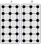
Figure 1: A partitioned finite spin system $A+B$. Solid lines represent the nearest neighbour coupling $J$ and dashed lines the interaction $K_{x,y}$ between the $2$ subsystems.

The system Hilbert space is ${\mathcal{H}}^{(L)}=\bigotimes_{x\in\Lambda_{L}}{\mathbb{C}}^{2}$. The Hamiltonian is that of an XY-spin model where the spins on $\Lambda_{L}^{-}$ do not interact with that on $\Lambda_{L}^{+}$ :

$$H^{(L)}=H^{(L,-)}+H^{(L,+)},$$

with

$$H^{(L,\pm)}=-\frac{J}{2}\sum_{x,y\text{ nearest}\atop\text{ neighbors in }\Lambda_{L}^{\pm}}\left(\sigma_{x}^{(1)}\sigma_{y}^{(1)}+\sigma_{x}^{(2)}\sigma_{y}^{(2)}\right),$$

where $J$ is a coupling constant. The interaction is

$$V^{(L)}=-\frac{1}{2}\sum_{x\in\Lambda_{L}^{-},y\in\Lambda_{L}^{+}}K_{x,y}(\sigma_{x}^{(1)}\sigma_{y}^{(1)}+\sigma_{x}^{(2)}\sigma_{y}^{(2)}),$$

where

$$K_{x,y}=\frac{\epsilon}{1+x_{2}^{2}}$$

if $x=(0,x_{2})\in\Lambda_{L}^{-}$ and $y=(1,x_{2})\in\Lambda_{L}^{+}$ and $K_{x,y}=0$ otherwise. The boundary between the two halves of the lattice is between the lines $x_{1}=0$ and $x_{1}=1$. Note that the interaction intensity decreases as one moves away from $(0,0)$. An assumption of this type is necessary if $V^{(L)}$ is to remain bounded in the thermodynamic limit $L\rightarrow\infty$.

For this model one can show that there exists $\alpha_{m}>0$ such that (5) holds and that our theorem applies. Hence we have inequality (7):

$$\mathbb{P}_{t}\left(\frac{|\Delta E|}{t}\geq\epsilon\right)\leq 2{\rm e}^{-t\epsilon\alpha_{m}+R(\alpha_{m})}$$

for any $\epsilon>0$.

Discussion.

Under a general condition on the regularity of the interaction evolution in imaginary time, we have proven a sharp form of the first law of thermodynamics for the FCS of energy variation.

Our result holds for any initial state of the system. If one assumes that systems $A$ and $B$ are initially in thermal equilibrium at temperatures $T_{A}$ and $T_{B}$, then the suppression of the fluctuations of the total energy current can be also proven by following the arguments of Andrieux et al. (2009).

Under additional assumptions it is possible to deal with cases where several reservoirs drive the joint system towards a non-equilibrium steady state and to derive properties of the joint distribution of the energy variations in each part of the system. A more strict condition on $R(\alpha)$ allows for the generalization of a symmetry of the limiting cumulant generating function proposed in Andrieux et al. (2009). Combined with time reversal invariance this leads to Onsager’s reciprocity relations. We investigate these topics in Benoist et al. (2015b).

In the present note we have limited ourselves to bounded interactions. The case of unbounded interactions (an example is the spin-boson model) is more technical and requires a separate analysis based on an application of Ruelle’s quantum transfer operators Jakšić et al. (2012). Although the physical picture emerging from this analysis is of an independent interest, the final results are much less general than in the case of bounded interactions De Roeck (2009); Jakšić et al. (2015).