Improving the INLA approach for approximate Bayesian inference for latent Gaussian models

Abstract

We introduce a new copula-based correction for generalized linear mixed models (GLMMs) within the integrated nested Laplace approximation (INLA) approach for approximate Bayesian inference for latent Gaussian models. While INLA is usually very accurate, some (rather extreme) cases of GLMMs with e.g. binomial or Poisson data have been seen to be problematic. Inaccuracies can occur when there is a very low degree of smoothing or “borrowing strength” within the model, and we have therefore developed a correction aiming to push the boundaries of the applicability of INLA. Our new correction has been implemented as part of the R-INLA package, and adds only negligible computational cost. Empirical evaluations on both real and simulated data indicate that the method works well.

1 Introduction

Integrated Nested Laplace Approximations (INLA) were introduced by Rue, Martino and Chopin (2009) as a tool to do approximate Bayesian inference in latent Gaussian models (LGMs). The class of LGMs covers a large part of models used today, and the INLA approach has been shown to be very accurate and extremely fast in most cases. Software is provided through the R-INLA package, see http://www.r-inla.org.

An important subclass of LGMs is the rich family of generalized linear mixed models (GLMMs) with Gaussian priors on fixed and random effects (Breslow and Clayton, 1993; McCulloch, Searle and Neuhaus, 2008). The use of INLA for Bayesian inference for GLMMs was investigated by Fong, Rue and Wakefield (2010), who reanalyzed all of the examples from Breslow and Clayton (1993). Fong, Rue and Wakefield (2010) found that INLA works very well in most cases, but one of their examples shows some inaccuracy for binary data with few or no replications. In this paper, we introduce a new correction term for INLA, significantly improving accuracy while adding negligibly to the overall computational cost.

Figure 1: Minimal example defined in Equation (1). The histograms show posterior distributions from a long MCMC run (ten chains of one million iterations each), the black curves show the posteriors from INLA, while the red curves show the posteriors using our new correction to INLA.

To set the scene, we consider a minimal simulated example illustrating the problem (postponing more thorough empirical evaluations until Section 3). Consider the following model: For $i=1,2,\ldots,n$, let $\mathrm{Prob}(y_{i}=0)=1-p_{i}$, $\mathrm{Prob}(y_{i}=1)=p_{i}$, and

$$\mathrm{logit}(p_{i})=\beta+u_{i},$$ (1)

where $u_{i}\sim N(0,\sigma^{2})$, iid. Let the precision $\sigma^{-2}$ have a $\mathrm{Gamma(1,1)}$ prior, while the prior for $\beta$ is $N(0,1)$. We simulated data from this model, setting $n=100$, $\sigma^{2}=1$ and $\beta=2$. Figure 1 shows the resulting posterior distributions for the intercept $\beta$ and for the log precision, $\log(\sigma^{-2})$, where the histograms show results from long MCMC runs using JAGS (Plummer, 2013), the black curves show posteriors from INLA without any correction, and the red curves show results using the new correction defined in Section 2. While some of our later examples show more dramatic differences between INLA and long MCMC runs, these results exemplify quite well our general experience with using INLA for “difficult” binary response GLMMs: Variances of both random and fixed effects tends to be underestimated, while the means of the fixed effects are reasonably well estimated.

Figure 2: Log-likelihood (top panel) and derivative of log-likelihood (bottom panel) for a single Bernoulli observation as a function of the linear predictor in a logistic model.

One part of the problem is that the usual assumptions ensuring asymptotic validity of the Laplace approximation do not hold here (for details on asymptotic results, see the discussion in Section 4 of Rue, Martino and Chopin (2009)). The independence of the random effects make the effective number of parameters (Spiegelhalter et al., 2002) on the order of the number of data points. In more complex models, there is often some amount of smoothing or replication that alleviates the problem, but it may still occur. Except in the case of spline smoothing models (Kauermann, Krivobokova and Fahrmeir, 2009), there is a lack of strong asymptotic results for random effects models with a large effective number of parameters. In the simulation from model (1), the data provide little information about the parameters, with the shape of the likelihood function adding to the problem. Figure 2 illustrates the general problem. Here, the top panel shows the log-likelihood of a single Bernoulli observation $Y$ as a function of the linear predictor $\eta$, i.e. $\log(\text{Prob}(Y=1))=\log(p)$ where $\text{logit}(p)=\eta$. The bottom panel shows the corresponding derivative. We see that the log-likelihood gets very flat (and the derivative near zero) for high values of $\eta$, so inference will get difficult.

Bayesian and frequentist estimation for GLMMs with binary outcomes has been given some attention in the recent literature (Capanu, Gönen and Begg, 2013; Grilli, Metelli and Rampichini, 2014; Sauter and Held, 2015), but a computationally efficient Bayesian solution appropriate for the INLA approach has been lacking. An alternative to our new approach would be to consider higher-order Laplace approximations (Shun and McCullagh, 1995; Raudenbush, Yang and Yosef, 2000; Evangelou, Zhu and Smith, 2011), other modifications to the Laplace approximation (Ruli, Sartori and Ventura, 2015; Ogden, 2015), or expectation propagation-type solutions (Cseke and Heskes, 2010), but we view them as too costly to be applicable for general use in INLA. The motivation for using INLA is speed, so we see it as a design requirement for any correction that it should add minimally to the running time of the algorithm.

We proceed as follows. In Section 2, we present a derivation of our new correction method. Section 3 presents empirical studies, both on real and simulated data, showing that the method works well in practice. Finally Section 4 gives a brief discussion and some concluding remarks.

2 Methodology

Consider a latent Gaussian model (Rue, Martino and Chopin, 2009), with hyperparameters $\theta=(\theta_{1},\ldots,\theta_{p})^{\prime}$, latent field $x=(x_{1},\ldots,x_{n})^{\prime}$ and observed data $y=\{y_{i}:i\in\mathcal{I}\}$ (for $\mathcal{I}\subseteq\{1,\ldots,n\}$), where the joint distribution may be written as

$$\pi({x},{\theta},{y})=\pi({\theta})\pi({x}|{\theta})\prod_{i\in\mathcal{I}}\pi(y_{i}|x_{i},{\theta})$$

where $\pi({x}|{\theta})$ is a multivariate Gaussian density. We want to approximate the posterior marginals $\pi(x_{i}|y)$ and $\pi(\theta_{j}|y)$. The Laplace approximation of $\tilde{\pi}(\theta|y)$ is

$$\tilde{\pi}(\theta|y)\propto\left.\frac{\pi(x,\theta,y)}{\tilde{\pi}_{G}(x|\theta,y)}\right|_{x=\mu(\theta)}$$ (2)

where $\tilde{\pi}_{G}({x}|{\theta},{y})$ is a Gaussian approximation found by matching the mode and the curvature at the mode of $\pi(x|\theta,y)$, and $\mu(\theta)$ is the mean of the Gaussian approximation.

Given $\tilde{\pi}(\theta|y)$ and some approximation $\tilde{\pi}(x_{i}|\theta,y)$ (see below), the posterior marginals of interest are calculated using numerical integration:

$$\tilde{\pi}(\theta_{j}|y) = \int\tilde{\pi}(\theta|y)\mathrm{d}\theta_{-j},$$

$$\tilde{\pi}(x_{i}|y) = \int\tilde{\pi}(x_{i}|\theta,y)\tilde{\pi}(\theta|y)\mathrm{d}\theta.$$ (3)

In the current implementation of INLA, the $\tilde{\pi}(x_{i}|\theta,y)$ used in (3) are approximated using skew normal densities $\tilde{\pi}_{\text{SN}}(x_{i}|\theta,y)$ (Azzalini and Capitanio, 1999), based on a second Laplace approximation; see Section 3.2.3 of Rue, Martino and Chopin (2009) for details. Notice that, in Equation (2) we use a Gaussian approximation $\tilde{\pi}_{G}({x}|{\theta},{y})$, with marginals $\tilde{\pi}_{G}({x_{i}}|{\theta},{y}),\ i=1,\ldots,n$. Thus, both $\pi_{\text{SN}}(x_{i}|\theta,y)$ and $\tilde{\pi}_{G}({x}|{\theta},{y})$ are approximations to the marginals $\pi(x_{i}|\theta,y)$, but the $\pi_{\text{SN}}(x_{i}|\theta,y)$ are more accurate since they are based on a second Laplace approximation. In (2) we need to approximate the full joint distribution $\pi(x|\theta,y)$. Our basic idea is to use the improved approximations $\tilde{\pi}_{SN}(x_{i}|\theta,y)$ in order to construct a better approximation to the joint distribution $\pi(x|\theta,y)$. We aim for an approximation of $\pi(x|\theta,y)$ that retains the dependence structure of the Gaussian approximation $\tilde{\pi}_{G}(x|\theta,y)$, while having the improved marginals $\tilde{\pi}_{SN}(x_{i}|\theta,y)$. This can be achieved by using a Gaussian copula.

Before we describe the copula construction, we need to define some notation. First, for $i=1,\ldots,n$, let $\tilde{\mu}_{i}(\theta)$ and $\tilde{\sigma}_{i}^{2}(\theta)$ denote the mean and variance of each marginal $\tilde{\pi}_{SN}(x_{i}|\theta,y)$, and let $F_{i}$ be the cumulative distribution function corresponding to $\tilde{\pi}_{SN}(x_{i}|\theta,y)$. Second, let $\tilde{x}_{i}\sim F_{i}$ and assume that $\tilde{F}_{i}$ is the distribution of $\tilde{z}_{i}=(\tilde{x}_{i}-\tilde{\mu}_{i}(\theta))/\sigma_{i}(\theta)$. As usual, $\Phi$ denotes the cumulative standard Gaussian distribution function. Furthermore, let $\mu_{i}(\theta)$ and $\sigma_{i}^{2}(\theta)$ denote the marginal means and variances of the Gaussian approximation $\tilde{\pi}_{G}({x}|{\theta},{y})$, let $Q(\theta)$ be the precision matrix of $\tilde{\pi}_{G}({x}|{\theta},{y})$, and let $x=(x_{1},\ldots,x_{n})$ where $x\sim\tilde{\pi}_{G}({x}|{\theta},{y})$, and define $z_{i}=(x_{i}-\mu_{i}(\theta))/\sigma_{i}(\theta),\ i=1,\ldots,n$. Note that we have $\tilde{\sigma}_{i}^{2}(\theta)\equiv\sigma_{i}^{2}(\theta)$ from the definition of $\tilde{\pi}_{SN}(x_{i}|\theta,y)$ (the construction of the skew normal changes the mean and adds skewness, but keeps the variance unchanged; again, see Section 3.2.3 of Rue, Martino and Chopin (2009) for detailed explanations), so from here on we denote both simply by $\sigma_{i}^{2}(\theta)$.

We will now show how to construct a joint distribution having marginals $F_{i}$ and the dependence structure from $\tilde{\pi}_{G}(x|\theta,y)$, using a Gaussian copula (see e.g. Nelsen (2007) for a general introduction). First, note that $\Phi(z_{i})\sim\text{U}[0,1]$ by the probability integral transform (PIT). Let $\tilde{z}_{i}=\tilde{F}_{i}^{-1}(\Phi(z_{i}))$. Applying the inverse of the PIT then yields that $\tilde{z}_{i}\sim\tilde{F}_{i}$, from which it follows that $\tilde{x}_{i}=\sigma_{i}(\theta)\tilde{z}_{i}+\tilde{\mu}_{i}(\theta)$ is distributed as $\tilde{x}_{i}\sim F_{i}$, which is the marginal distribution we want. Since we have only done marginal transformations, the dependence structure of the original $x=(x_{1},\ldots x_{n})^{\prime}$ is still intact. Thus, to construct the new approximation to the joint distribution $\tilde{\pi}(x|\theta,y)$, we define the transformed value $\tilde{x}_{i}$ as follows:

$$\tilde{x}_{i}=\sigma_{i}(\theta)\tilde{F}_{i}^{-1}\left[\Phi\left(\frac{x_{i}-\mu_{i}(\theta)}{\sigma_{i}(\theta)}\right)\right]+\tilde{\mu}_{i}(\theta).$$ (4)

We may simplify the construction above by replacing the $\tilde{F}_{i}$ in (4) by $\Phi$. This means that we do not correct for skewness, but we take advantage of the improved mean $\tilde{\mu}_{i}(\theta)$ from $\tilde{\pi}_{SN}(x_{i}|\theta,y)$. We denote this as the “mean only” correction. (We will later discuss the possibility of retaining $\tilde{F}_{i}$ as a skew normal; this we denote as the “mean and skewness” correction.) In the simple “mean only” case, the transformation reduces to a shift in mean:

$$\tilde{x}_{i}=x_{i}-\mu_{i}(\theta)+\tilde{\mu}_{i}(\theta),$$

the Jacobian is equal to one, and the transformed joint density function is a multivariate normal with mean $\tilde{\mu}$ and precision matrix $Q$, i.e.

$$\log\tilde{\pi}(\tilde{x}|\theta,y)=\frac{1}{2}\log|Q(\theta)|-\frac{1}{2}(\tilde{x}-\tilde{\mu}(\theta))^{\prime}Q(\theta)(\tilde{x}-\tilde{\mu}(\theta))+\text{constant}$$ (5)

In the Laplace approximation defined in Equation (2), both the numerator and the denominator should be evaluated in the point $\tilde{x}=\mu(\theta)$, where $\mu(\theta)=(\mu_{1}(\theta),\ldots,\mu_{n}(\theta))^{\prime}$ is the mean of the Gaussian approximation $\tilde{\pi}_{G}(x|\theta,y)$. Thus, the density functions above should be evaluated in $\tilde{x}=\mu(\theta)$. From Equation (2), the original (uncorrected) log posterior is

$$\log\tilde{\pi}(\theta|y)=\log\pi({x},{\theta},{y})-\log\tilde{\pi}_{G}({x}|{\theta},{y})+\text{constant}$$ (6)

evaluated at $x=\mu(\theta)$, where

$$\left.\log\tilde{\pi}_{G}({x}|{\theta},{y})\right|_{x=\mu(\theta)}=\frac{1}{2}\log|Q(\theta)|+\text{constant},$$ (7)

Comparing equations (5), (6), and (7), we see that the copula approximation can be implemented by adding the term $C(\theta)$ to the already calculated log posterior evaluated at $\mu(\theta)$, where

$$C(\theta)=\frac{1}{2}(\mu(\theta)-\tilde{\mu}(\theta))^{\prime}Q(\theta)(\mu(\theta)-\tilde{\mu}(\theta)).$$

The addition of the term $C(\theta)$ does not add significantly to the computational cost of INLA — this simple operation is essentially free.

For the INLA implementation of the copula correction, we have found that it is sufficient to only include fixed effects (including any random effects of length one) in the calculation of $C(\theta)$. The effect of the correction is strongest and most consistent for the fixed effects, while the (often very numerous) random effects contribute very small individual effects to the correction, mainly adding extraneous noise to the estimation. For these reasons, including only fixed effects gives better numerical stability and also seems to provide a more accurate approximation, while reducing computational costs. Conceptually, including only the fixed effects involves finding $\Sigma(\theta)=Q(\theta)^{-1}$, and then again finding $Q_{\mathcal{J}}(\theta)=\Sigma_{\mathcal{J}}(\theta)^{-1}$ (where $\mathcal{J}$ is the index set of the fixed effects), which might seem computationally costly. However, it can be done cheaply by using the linear combination feature described in Section 4.4 of Martins et al. (2013): If $n_{f}$ is the number of fixed effects, only the (parallel) solution of a $n_{f}$-dimensional linear system is needed.

Additionally, to guard against over-correction, we perform a soft thresholding on $C(\theta)$, as follows: First we define a sigmoidal function $f(t)$:

$$f(t)=\frac{2}{1+\exp(-2t)}-1,$$

which is increasing, has derivative equal to one at the point $t=0$, and where $f(t)\rightarrow 1$ as $t\rightarrow\infty$. Then we replace $C(\theta)$ by $C_{t}(\theta)$, where

$$C_{t}(\theta)=uf(C(\theta)/u),$$

for $u=n_{f}\xi$ and with the “correction factor” parameter $\xi>0$ determining the degree of shrinkage (more shrinkage for smaller values of $\xi$). Since the function $f(t)$ is approximately linear with unit slope around zero, $C_{t}(\theta)$ will be close to $C(\theta)$ for small and moderate values of $C(\theta)$, while larger values will be increasingly shrunk toward zero. Note that since $f(t)<1$ for all $t$, $C_{t}(\theta)<u$. The value of $\xi$ does not have a large impact on the results unless a too small value is chosen. Its main purpose is as a safeguard to avoid too large corrections in very difficult cases. In our experience $\xi=1$ gives too strong shrinkage, while for example $\xi=100$ corresponds to no shrinkage, so it seems clear that $\xi$ should be somewhere in between these extremes. We have found that $\xi=10$ is a good choice, letting the correction do its job while guarding against too large changes, and we have used this value for all of the examples. Results appear to be very robust to the exact value chosen for $\xi$. Note also that since the correction effect $u$ is scaled with the number $n_{f}$ of fixed effects, it is less surprising that a single value for $\xi$ could work well in a wide variety of circumstances.

As mentioned, we have also investigated a more general case of the copula construction, where we retain $F_{i}$ as a skew normal distribution, i.e. the CDF of $\tilde{\pi}_{SN}(x_{i}|\theta,y)$. This results in a more complicated correction term $C_{\text{skew}}(\theta)$, derived in Appendix A. We have not found any appreciable differences in the accuracy compared to the simpler case without skewness, so we have concluded that the non-skew version is preferable due to its simplicity. We will show both the skew and the non-skew correction for the toenail data discussed in Section 3.2, but otherwise we show only results from the simpler non-skew version. We have tried both corrections on many (both real and simulated) data sets, and never seen a significant difference in the results.

3 Empirical results

3.1 Have we solved the problems detected by Fong et al. (2010)?

As mentioned in the Introduction, Fong, Rue and Wakefield (2010) studied the use of INLA for binary valued GLMMs, and they showed that the approximations were inaccurate in some cases. We have redone the simulation experiment described on pages 10–14 of the Supplementary Material of Fong, Rue and Wakefield (2010), both for INLA without any correction, and INLA with the “mean only” correction described in Section 2.

In the original simulation study by Fong, Rue and Wakefield (2010), $Y_{ij}$ are iid $\mathrm{Binomial}(m,p_{ij})$, with $i=1,\ldots,100$ clusters, $j=1,\ldots,7$ observations per cluster, and $m\in\{1,2,4,8\}$. Given $x_{i}=0$ for $i\leq 50$ and $x_{i}=1$ otherwise, and sampling times $t=(t_{1},\ldots,t_{7})^{\prime}=(-3,-2,-1,0,1,2,3)^{\prime}$, the following two models were considered:

$$\text{logit}\ p_{ij} = \beta_{0}+\beta_{1}t_{j}+\beta_{2}x_{i}+\beta_{3}t_{j}x_{i}+b_{0i}$$ (8)

$$\text{logit}\ p_{ij} = \beta_{0}+\beta_{1}t_{j}+\beta_{2}x_{i}+\beta_{3}t_{j}x_{i}+b_{0i}+b_{1i}t_{j},$$ (9)

which corresponds to models (0.7) and (0.8) on page 11 of the Supplementary Material of Fong, Rue and Wakefield (2010).

We first consider model (8). We only show the results for $m=1$ (i.e. binary data), as this is the most difficult case with the largest errors in the approximation. The correction also works well for $m>1$, but this case is easier to deal with for INLA. This is seen empirically, and is also as expected based on considering the asymptotic properties of the Laplace approximation: for $m>1$ there is more “borrowing of strength”/replication, so the original approximation should work better. We use the same settings as Fong, Rue and Wakefield (2010): $b_{0i}\sim_{iid}N(0,\sigma_{0}^{2})$ where $\sigma_{0}^{2}=1$, the prior $\text{Gamma}(0.5,0.0164)$ for $\sigma_{0}^{-2}$ and $N(0,1000)$ priors for the $\beta_{i}$. The true values of the fixed effects are $\beta=(\beta_{0},\beta_{1},\beta_{2},\beta_{3})^{\prime}=(-2.5,1.0,-1.0,-0.5)^{\prime}$. We made 1,000 simulated data sets, running INLA both with and without the new correction, as well as very long MCMC chains using JAGS (each of the 1,000 datasets were run with 1,000,000 MCMC samples after a burn-in of 100,000, using every 100th sample).

Table 1: Results from simulation study from model (8)

Averages of posterior means:
		$\sigma_{0}^{2}$	$\sigma_{0}$	$\log\sigma_{0}^{-2}$	$\beta_{0}$	$\beta_{1}$	$\beta_{2}$	$\beta_{3}$
	True values	1.000	1.000	0.000	-2.500	1.000	-1.000	-0.500
	Uncorrected INLA	0.705	0.722	1.133	-2.494	0.998	-1.052	-0.486
	Corrected INLA	0.952	0.850	0.775	-2.562	1.024	-1.080	-0.504
	MCMC	0.946	0.849	0.773	-2.537	1.017	-1.081	-0.482
Comparison between INLA and MCMC, (E(INLA)-E(MCMC))/sd(MCMC):
		$\sigma_{0}^{2}$	$\sigma_{0}$	$\log\sigma_{0}^{-2}$	$\beta_{0}$	$\beta_{1}$	$\beta_{2}$	$\beta_{3}$
	Uncorrected INLA	-0.382	-0.403	0.390	0.120	-0.127	0.052	-0.016
	Corrected INLA	-0.003	0.000	0.002	-0.073	0.046	-0.002	-0.101
Ratio of variances, Var(INLA)/Var(MCMC):
		$\sigma_{0}^{2}$	$\sigma_{0}$	$\log\sigma_{0}^{-2}$	$\beta_{0}$	$\beta_{1}$	$\beta_{2}$	$\beta_{3}$
	Uncorrected INLA	0.585	0.812	1.174	0.822	0.834	0.882	0.889
	Corrected INLA	0.933	0.956	0.998	0.904	0.871	0.943	0.908
Average coverage of 95% intervals from INLA over MCMC samples:
		$\sigma_{0}^{2}$	$\sigma_{0}$	$\log\sigma_{0}^{-2}$	$\beta_{0}$	$\beta_{1}$	$\beta_{2}$	$\beta_{3}$
	Uncorrected INLA	90.3%	90.0%	90.8%	92.6%	92.7%	93.5%	93.5%
	Corrected INLA	94.2%	93.9%	94.4%	93.5%	93.1%	94.3%	93.7%

Results from the simulation study are shown in Table 1. Note that the aim here is to be as close as possible to the MCMC results, not the true values. The upper part of the table shows averages of the posterior means over the 1,000 simulations. We see that INLA gets much closer to the MCMC results for all parameters except $\beta_{3}$, which is in any case reasonably close to the MCMC value. The improvement is particularly large for the variance parameter. This is also seen in the second panel, which shows $(\text{E}(\theta^{\text{INLA}}|y)-\text{E}(\theta^{\text{MCMC}}|y))/\text{sd}(\theta^{\text{MCMC}}|y)$ for each parameter $\theta$ (averaged over the 1,000 simulations), i.e. the difference in INLA and MCMC estimates scaled by the MCMC standard deviation. Here, the random effects variance and the fixed effects except $\beta_{3}$ are also more accurately estimated. The third lower panel shows the ratios $\text{Var}(\theta^{\text{INLA}}|y)/\text{Var}(\theta^{\text{MCMC}}|y)$; here the correction improves the estimation of the variance for all parameters. For $\sigma_{0}^{2}$, $\sigma_{0}$ and $\log\sigma_{0}^{-2}$ we get very close to a ratio of one, and there are also major improvements for the fixed effects variances. Finally, the bottom panel shows average coverage of 95% (i.e., $(q_{0.025},q_{0.975})$) credible intervals from INLA over the MCMC samples for each simulated data set. Clearly, coverage is improved considerably by the correction. Table 2 reports summary statistics for the computation times in seconds over the 1,000 data sets. Note that in this case computational times are abnormally high due to somewhat extreme parameter settings – INLA will usually be much faster. However, ratios of computing times for the corrected vs the uncorrected versions should stay approximately the same.

Appendix B contains additional simulation studies: Results from simulations for model (9) for different values of the covariance matrix of $(b_{0i},b_{1i})^{\prime}$ are shown in Appendix B.1. Furthermore, in Appendix B.2 we consider the effect of having extremely few observations per cluster, while we in Appendix B.3 study a misspecified model, simulating from model (9) while estimating model (8). The correction appears to work well for all the different cases considered in Appendix B.

Table 2: Summary statistics for computation times in seconds for each data set

	Min.	1st Qu.	Median	Mean	3rd Qu.	Max.
Uncorrected INLA	1.70	2.25	2.39	2.43	2.56	3.41
Corrected INLA	1.77	2.58	2.69	2.74	2.86	3.89

Figure 3: The top panel shows the posterior density of the hyperparameter (log precision) for the toenail data. The histogram is from one million MCMC samples from JAGS, the blue curve is from uncorrected INLA, the red curve from INLA with the “mean only” correction, and the green curve from INLA with the “mean and skewness” correction. The bottom panel shows the additive corrections to the log posterior for the toenail data for the “mean only” and the “mean and skewness” correction.

3.2 What happens when the random effects variance increases?

We start by discussing the toenail data, which is a classical data set with a binary response and repeated measures (De Backer et al., 1998; Lesaffre and Spiessens, 2001). The data are from a clinical trial comparing two competing treatments for toenail infection (dermatophyte onychomycosis). The 294 patients were randomized to receive either itraconazole or terbinafine, and the outcome (either “not severe” infection, coded as $0$, or “severe” infection, coded as $1$) was recorded at seven follow-up visits. Not all patients attended all the follow-up visits, and the patients did not always appear at the scheduled time. The exact time of the visits (in months since baseline) was recorded. For individual $i$, visit $j$, with outcome $y_{ij}$, treatment $\text{Trt}_{i}$ and time $\text{Time}_{ij}$ our model is then

$$y_{ij} \sim \text{Bernoulli}(p_{ij})$$

$$\text{logit}\ p_{ij} = \alpha_{0}+\alpha_{\text{Trt}}\text{Trt}_{i}+\alpha_{\text{Time}}\text{Time}_{ij}+\alpha_{TT}\text{Trt}_{i}\text{Time}_{ij}+b_{i}$$

$$b_{i} \sim N(0,\sigma^{2}).$$

Notice that this is the same model as model (8), except that the time variable here varies over individuals. Normal priors with mean zero and variance $10^{4}$ were used for $\alpha_{0}$, $\alpha_{\text{Trt}}$, $\alpha_{\text{Time}}$, and $\alpha_{TT}$. INLA underestimates $\sigma^{2}$ quite severely. The top panel of Figure 3 shows the different estimates of the posterior distribution of the log precision, $\log\sigma^{-2}$. The histogram shows the results from a long MCMC run using JAGS, the black curve shows the posterior from INLA without the correction, the red curve shows the simple (non-skew) version of the INLA correction, while the green curve shows the INLA correction accounting for skewness (as discussed in Appendix A). The bottom panel of Figure 3 shows the additive correction to the log posterior density, as a function of the hyperparameter (log precision). We see that there is very little difference between the two corrections.

For the toenail data, the estimated random effects standard deviation is approximately $\sigma=4$, which is very high. To investigate how the copula correction works as $\sigma$ increases, we studied simulated data sets from the model above, where we set $\sigma$ to different values, and where the $\alpha$ parameters were fixed to the values from a long MCMC run using the real toenail data (i.e., we simulate only the outcome, keeping the covariates unchanged). Results are shown in Figure 4 for different values of $\sigma$ ranging from $\sigma=1$ to $\sigma=16$. We clearly get very accurate corrected posteriors for $\sigma<4$. For $\sigma\geq 4$, we gradually get a tendency of under-correction.

Figure 4: Posteriors densities of log precision from the toenail simulation experiment for different values of the random effects standard deviation $\sigma$ (the value of $\sigma$ is shown above each histogram). The histograms are from long MCMC runs, uncorrected INLA are shown as black curves, while the red curves shows INLA with the correction. Since the goal here is to study the difference between MCMC and INLA, we omit axes – the relevant scale is given by the MCMC variances, which are evident from the histograms.

3.3 Simulated example with Poisson likelihood

We shall now study the case where the data are Poisson distributed. We consider a simple simulated (extreme) example in order to investigate how well the correction works in the Poisson case. For $i=1,\ldots,n$ we generated iid $y_{i}\sim\text{Poisson}(\mu_{i})$ where

$$\log(\mu_{i})=\beta+u_{i},$$

with $u_{i}\sim N(0,\sigma^{2})$. We chose $n=300$ and $\sigma^{2}=1$, a $\text{Gamma}(1,1)$ prior for the precision $\sigma^{-1}$, and a $N(0,1)$ prior for $\beta$. Figure 5 shows the results for different values of the intercept $\beta$. Each histogram is based on ten parallell MCMC runs using JAGS, each with 200,000 iterations after a burn-in of 100,000. Here, reduction of $\beta$ implies that estimation is more difficult, since negative $\beta$ with large absolute value will imply that the counts $y_{i}$ are very low, with many zeroes, and the data are uninformative. We see that uncorrected INLA tends to get less accurate as $\beta$ moves towards more extreme values, while the correction seems to work well.

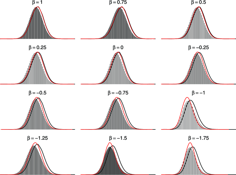
Figure 5: Posteriors densities of log precision from the Poisson simulation experiment for different values of the intercept $\beta$ (the value of $\beta$ is shown above each histogram). The histograms are from long MCMC runs, uncorrected INLA posteriors are shown as black curves, while the red curves shows INLA posteriors with the correction.

3.4 What if the latent structures are more complicated?

Until now, we have considered fairly simple latent structures, where the random effects have been iid (multivariate) normally distributed. The reader may perhaps wonder if the generality implied by having “latent Gaussian models” in the title is really justified – what if latent structures are more complicated, with for example temporal or spatial structure?

In fact, the complexity of the latent field is not particularly relevant for the accuracy problems we study here. This can be seen by considering the basic formulation of the latent Gaussian model together with the main building blocks of the INLA machinery: Essentially, the latent structure is contained within the Gaussian part, for which the computations are exact (and fast, since the precision matrix of the Gaussian part will usually be sparse). In a sense, the LGM approach separates the estimation in an “easy” (Gaussian) part and a “difficult” part. It is perhaps somewhat counterintuitive at first sight that the dynamic/time-series/spatial model constitutes the “easy” part! In this paper we have in fact considered the “difficult” part, aiming to choose examples at the boundary of what we considered to be feasible. Thus, we argue that our general title is indeed justified.

We illustrate this with a simple simulated example where the latent structure is auto-regressive of order one (AR1), using a similar setup as in the “minimal” example presented in the Introduction. For $i=1,2,\ldots,n$, let $\mathrm{Prob}(y_{i}=0)=1-p_{i}$, $\mathrm{Prob}(y_{i}=1)=p_{i}$, and

$$\mathrm{logit}(p_{i})=\beta+u_{i},$$ (10)

where the $u_{i}$ are now given an AR1 model, as follows: $u_{1}\sim N(0,\kappa^{-1})$, $u_{i}=\rho u_{i-1}+\varepsilon_{i}$ (where $\varepsilon_{i}\sim N(0,\tau^{-1})$) for $i=2,3,\ldots,n$, where $\kappa=\tau(1-\rho^{2})$ is the marginal precision. Define

$$\theta_{1}=\log(\kappa)$$

and

$$\theta_{2}=\log\left(\frac{1+\rho}{1-\rho}\right)$$

which is the parameterization used internally in INLA. We use a Gamma$(1,1)$ prior for $\kappa$, and $N(0,1)$ priors for both $\beta$ and $\theta_{2}$. Data was simulated from model (10), using $\rho=0.5$, $\tau=1$ and $\beta=2$ as the true values. As in the example in the Introduction, we made long MCMC runs and compared the results to INLA both with and without the correction. The results are shown in Figure 6. Again, it is clear that the overall accuracy of INLA is improved using the correction.

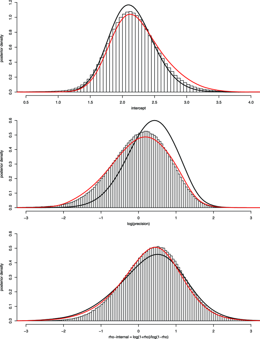
Figure 6: AR1 example defined in Equation (10). The top panel displays results for the intercept parameter $\beta$, the middle panel shows results for $\theta_{1}=log(\kappa)$, and the bottom panel show results for $\theta_{2}=\log\left(\frac{1+\rho}{1-\rho}\right)$, the “internal $\rho$” of INLA. The histograms show posterior distributions from a long MCMC run (ten chains of one million iterations each), the black curves show the posterior from INLA, while the red curve shows the posteriors using our new correction to INLA.

4 Discussion

The binary (and, more generally, binomial) GLMMs discussed in Sections 3.1 and 3.2 are are important in many applications, particularly for biomedical data. Poisson GLMMs are also of great interest, and among the difficult cases here are point processes such as log-Gaussian Cox processes (Illian, Sørbye and Rue, 2012; Simpson et al., 2013), where data are typically extremely sparse: essentially there are ones at the observed points, and zeroes everywhere else. Our example in Section 3.3 shows a stylized, extreme case of this type. Studying the correction for the full log-Gaussian Cox process case could be a topic for future work. Even though the point process case may be difficult, there will often be some degree of smoothing and/or replication making inference easier, so real data sets should be less extreme than the simulated example in Section 3.3.

From the results in this paper, it appears that the copula correction is robust and works well. There is no general theory guaranteeing that the method will always work under all circumstances, but we feel that the intuition underlying the method is quite strong. Since INLA for LGMs is quite accurate in most cases, the correction is not needed in general, only for problematic cases such as those discussed in this paper. Using the copula correction method, we can stretch the limits of applicability of INLA, while maintaining its computational speed.

Appendix A Copula correction accounting for skewness

Let $\tilde{F}_{i}$ denote the “standardized” skew normal CDF corresponding to$\tilde{\pi}_{SN}(x_{i}|\theta,y)$. We start by finding the Jacobian of the transformation defined in Equation (4). Note first that, immediately from (4)

$$\tilde{F}_{i}\left(\frac{\tilde{x}_{i}-\tilde{\mu}_{i}(\theta)}{\sigma_{i}(\theta)}\right)=\Phi\left(\frac{x_{i}-\mu_{i}(\theta)}{\sigma_{i}(\theta)}\right).$$

Letting $\tilde{f}_{i}$ and $\phi$ denote the density functions corresponding to $\tilde{F}_{i}$ and $\Phi$, differentiating with respect to $\tilde{x}_{i}$ then gives

$$\tilde{f}_{i}\left(\frac{\tilde{x}_{i}-\tilde{\mu}_{i}(\theta)}{\sigma_{i}(\theta)}\right)\frac{1}{\sigma_{i}(\theta)}=\phi\left(\frac{x_{i}-\mu_{i}(\theta)}{\sigma_{i}(\theta)}\right)\frac{\partial x_{i}}{\partial\tilde{x}_{i}}\frac{1}{\sigma_{i}(\theta)}$$

so

$$\frac{\partial x_{i}}{\partial\tilde{x}_{i}}=\frac{\tilde{f}_{i}\left(\frac{\tilde{x}_{i}-\tilde{\mu}_{i}(\theta)}{\sigma_{i}(\theta)}\right)}{\phi\left(\frac{x_{i}-\mu_{i}(\theta)}{\sigma_{i}(\theta)}\right)}=\frac{\tilde{f}_{i}\left(\frac{\tilde{x}_{i}-\tilde{\mu}_{i}(\theta)}{\sigma_{i}(\theta)}\right)}{\phi\left(\Phi^{-1}\left[\tilde{F}_{i}\left(\frac{\tilde{x}_{i}-\tilde{\mu}_{i}(\theta)}{\sigma_{i}(\theta)}\right)\right]\right)}$$

and the Jacobian of the transformation is $\prod_{i=1}^{n}\frac{\partial x_{i}}{\partial\tilde{x}_{i}}$ since $\frac{\partial x_{i}}{\partial\tilde{x}_{j}}=0$ for $i\neq j$ and $\frac{\partial x_{i}}{\partial\tilde{x}_{i}}\geq 0$ for all $i$.

Note that $(x-\mu(\theta))^{\prime}Q(\theta)(x-\mu(\theta))=\sum_{i=1}^{n}\sum_{j=1}^{n}Q_{ij}(\theta)(x_{i}-\mu_{i}(\theta))(x_{j}-\mu_{j}(\theta))$ where $Q(\theta)=(Q_{ij}(\theta))$. Collecting the different terms and again substituting

$$\frac{x_{i}-\mu_{i}(\theta)}{\sigma_{i}(\theta)}=\Phi^{-1}\left[\tilde{F}_{i}\left(\frac{\tilde{x}_{i}-\tilde{\mu}_{i}(\theta)}{\sigma_{i}(\theta)}\right)\right],$$

the transformed joint log density $\tilde{\pi}(\tilde{x}|\theta,y)$ is therefore

$$\log\tilde{\pi}(\tilde{x}|\theta,y)=\frac{1}{2}\log|Q(\theta)|$$

$$-\frac{1}{2}\sum_{i=1}^{n}\sum_{j=1}^{n}Q_{ij}(\theta)\sigma_{i}(\theta)\sigma_{j}\Phi^{-1}\left[\tilde{F}_{i}\left(\frac{\tilde{x}_{i}-\tilde{\mu}_{i}(\theta)}{\sigma_{i}(\theta)}\right)\right]\Phi^{-1}\left[\tilde{F}_{j}\left(\frac{\tilde{x}_{j}-\tilde{\mu}_{j}(\theta)}{\sigma_{j}(\theta)}\right)\right]$$

$$+\sum_{i=1}^{n}\log\tilde{f}_{i}\left(\frac{\tilde{x}_{i}-\tilde{\mu}_{i}(\theta)}{\sigma_{i}(\theta)}\right)-\sum_{i=1}^{n}\log\phi\left(\Phi^{-1}\left[\tilde{F}_{i}\left(\frac{\tilde{x}_{i}-\tilde{\mu}_{i}(\theta)}{\sigma_{i}(\theta)}\right)\right]\right)+\text{constant}$$

The original (uncorrected) log posterior is

$$\log\tilde{\pi}(\theta|y)=\log\pi({x},{\theta},{y})-\log\tilde{\pi}_{F}({x}|{\theta},{y})+\text{constant},$$

evaluated at $x=\mu(\theta)$ where $\left.\log\tilde{\pi}_{F}({x}|{\theta},{y})\right|_{x=\mu(\theta)}=\frac{1}{2}\log|Q(\theta)|+\text{constant}$. Therefore, the version of the copula correction accounting for skewness amounts to adding a term $C_{\text{skew}}(\theta)$ to the original log joint posterior, where

$$C_{\text{skew}}(\theta)=$$

$$\frac{1}{2}\sum_{i=1}^{n}\sum_{j=1}^{n}Q_{ij}(\theta)\sigma_{i}(\theta)\sigma_{j}(\theta)\Phi^{-1}\left[\tilde{F}_{i}\left(\frac{\mu_{i}(\theta)-\tilde{\mu}_{i}(\theta)}{\sigma_{i}(\theta)}\right)\right]\!\Phi^{-1}\!\left[\tilde{F}_{j}\left(\frac{\mu_{j}(\theta)-\tilde{\mu}_{j}(\theta)}{\sigma_{j}(\theta)}\right)\right]$$

$$+\sum_{i=1}^{n}\log\tilde{f}_{i}\left(\frac{\mu_{i}(\theta)-\tilde{\mu}_{i}(\theta)}{\sigma_{i}(\theta)}\right)-\sum_{i=1}^{n}\log\phi\left(\Phi^{-1}\left[\tilde{F}_{i}\left(\frac{\mu_{i}(\theta)-\tilde{\mu}_{i}(\theta)}{\sigma_{i}(\theta)}\right)\right]\right).$$

Calculations of $\tilde{F}_{i}$ and $\tilde{f}_{i}$ were done using the functions psn and dsn in the R package sn (Azzalini, 2015).

Appendix B Additional simulation results

B.1 Model with two dependent random effects

Here we study model (0.8) from page 11 of the Supplementary Material of Fong, Rue and Wakefield (2010), where the observations $Y_{ij}$ are iid Binomial$(p_{ij},m)$, with $i=1,\ldots,100$ clusters, $j=1,\ldots,7$ observations per cluster, $x_{i}=0$ for $i\leq 50$ and $x_{i}=1$ otherwise, and sampling times $t=(t_{1},\ldots,t_{7})^{\prime}=(-3,-2,-1,0,1,2,3)^{\prime}$. The model is

$$\text{logit}\ p_{ij}=\beta_{0}+\beta_{1}t_{j}+\beta_{2}x_{i}+\beta_{3}t_{j}x_{i}+b_{0i}+b_{1i}t_{j},$$ (11)

where the $(b_{0i},b_{1i})^{\prime}$ are iid bivariate normally distributed with mean $(0,0)$. Following Fong, Rue and Wakefield (2010), the prior for the precision matrix of $(b_{0i},b_{1i})^{\prime}$ is a Wishart distribution with three degrees of freedom and diagonal scale parameter with diagonal elements $0.17$ and $0.025$. The fixed effects are given $N(0,1000)$ priors.

As in Fong, Rue and Wakefield (2010), we shall consider the case when $b_{0i}$ and $b_{1i}$ are uncorrelated, but we shall here also consider the correlated case with correlation $\rho=0.5$ and $\rho=0.9$, respectively. Additionally, we consider two different settings of the marginal variances of $b_{0i}$ and $b_{1i}$:

1. Var$(b_{0i})=0.5$, Var$(b_{1i})=0.25$ (as in Fong, Rue and Wakefield (2010)),

2. Var$(b_{0i})=3.0$, Var$(b_{1i})=0.5$.

For each of the two settings of the marginal variances above, we ran the simulation experiment for the three settings of $\rho$ ($0$, $0.5$ and $0.9$ correlation), giving six simulation settings in total. For each simulation setting, we made 200 simulated data sets, and ran two MCMC chains of 200,000 iterations each (after discarding the first 100,000 iterations) for each simulated data set.

We have yet to specify the number of trials $m$ in the binomial distribution. It turns out that this model is nearly unidentifiable for $m=1$, with very slow MCMC convergence and with numerical instability when running INLA (both with and without the correction). Therefore, we will here consider $m>1$, and show the results for $m=2$. Results (not shown) are similar also for $m>2$. As expected, the estimation becomes more accurate as $m$ grows, and for large $m$ (say, $m\geq 10$) there is no need for the INLA correction anymore.

Results are shown in Tables 3–8 below, where we use the parameterization $(\theta_{1},\theta_{2},\theta_{3})$ used internally by INLA, where $\theta_{1}=\log(\sigma_{0}^{-2})$, $\theta_{2}=\log(\sigma_{1}^{-2})$ and $\theta_{3}=\log\left(\frac{1+\rho}{1-\rho}\right)$ (note that $\theta_{1}$, $\theta_{2}$ and $\theta_{3}$ are defined on the whole real line). It seems like the correction is working quite well, giving an overall improvement. The coverage probabilities are improved in all cases expect for the $\log\left(\frac{1+\rho}{1-\rho}\right)$ with $\rho\leq 0.5$, so we see an improvement for $38$ of the $6*7=42$ combinations of parameters and simulation settings. The variance ratio Var(INLA)/Var(MCMC) is also improved for nearly all the cases, while the other performance measures show an overall (though not uniform) improvement. The method does not seem to deteriorate for higher values of the marginal variances and correlation.

Table 3: Results from simulation study (11) with Var$(b_{0i})=0.5$, Var$(b_{1i})=0.25$ and $\rho=0$

Averages of posterior means:
		$\log(\sigma_{0}^{-2})$	$\log(\sigma_{1}^{-2})$	$\log\left(\frac{1+\rho}{1-\rho}\right)$	$\beta_{0}$	$\beta_{1}$	$\beta_{2}$	$\beta_{3}$
	True values	0.693	1.386	0.000	-2.500	1.000	-1.000	-0.500
	Uncorrected INLA	1.527	2.130	1.566	-2.664	1.021	-0.692	-0.428
	Corrected INLA	1.380	2.016	1.313	-2.703	1.038	-0.704	-0.429
	MCMC	1.449	2.022	1.707	-2.694	1.032	-0.707	-0.421
Comparison between INLA and MCMC, (E(INLA)-E(MCMC))/sd(MCMC):
		$\log(\sigma_{0}^{-2})$	$\log(\sigma_{1}^{-2})$	$\log\left(\frac{1+\rho}{1-\rho}\right)$	$\beta_{0}$	$\beta_{1}$	$\beta_{2}$	$\beta_{3}$
	Uncorrected INLA	0.113	0.167	-0.124	0.125	-0.086	0.042	-0.038
	Corrected INLA	-0.086	-0.028	-0.329	-0.028	0.045	0.007	-0.047
Ratio of variances, Var(INLA)/Var(MCMC):
		$\log(\sigma_{0}^{-2})$	$\log(\sigma_{1}^{-2})$	$\log\left(\frac{1+\rho}{1-\rho}\right)$	$\beta_{0}$	$\beta_{1}$	$\beta_{2}$	$\beta_{3}$
	Uncorrected INLA	0.882	0.986	0.927	0.905	0.907	0.937	0.948
	Corrected INLA	0.943	0.974	0.996	0.994	0.982	0.977	0.987
Average coverage of 95% intervals from INLA over MCMC samples:
		$\log(\sigma_{0}^{-2})$	$\log(\sigma_{1}^{-2})$	$\log\left(\frac{1+\rho}{1-\rho}\right)$	$\beta_{0}$	$\beta_{1}$	$\beta_{2}$	$\beta_{3}$
	Uncorrected INLA	92.4%	93.3%	92.8%	93.7%	93.7%	94.2%	94.3%
	Corrected INLA	92.9%	93.7%	90.0%	93.7%	93.8%	94.6%	94.7%

Table 4: Results from simulation study (11) with Var$(b_{0i})=0.5$, Var$(b_{1i})=0.25$ and $\rho=0.5$

Averages of posterior means:
		$\log(\sigma_{0}^{-2})$	$\log(\sigma_{1}^{-2})$	$\log\left(\frac{1+\rho}{1-\rho}\right)$	$\beta_{0}$	$\beta_{1}$	$\beta_{2}$	$\beta_{3}$
	True values	0.693	1.386	1.099	-2.500	1.000	-1.000	-0.500
	Uncorrected INLA	1.444	1.866	2.051	-2.623	1.139	-0.721	-0.590
	Corrected INLA	1.366	1.786	1.900	-2.642	1.148	-0.730	-0.594
	MCMC	1.363	1.790	2.176	-2.649	1.148	-0.731	-0.582
Comparison between INLA and MCMC, (E(INLA)-E(MCMC))/sd(MCMC):
		$\log(\sigma_{0}^{-2})$	$\log(\sigma_{1}^{-2})$	$\log\left(\frac{1+\rho}{1-\rho}\right)$	$\beta_{0}$	$\beta_{1}$	$\beta_{2}$	$\beta_{3}$
	Uncorrected INLA	0.126	0.134	-0.118	0.111	-0.073	0.027	-0.041
	Corrected INLA	0.013	-0.031	-0.252	0.035	-0.005	0.002	-0.066
Ratio of variances, Var(INLA)/Var(MCMC):
		$\log(\sigma_{0}^{-2})$	$\log(\sigma_{1}^{-2})$	$\log\left(\frac{1+\rho}{1-\rho}\right)$	$\beta_{0}$	$\beta_{1}$	$\beta_{2}$	$\beta_{3}$
	Uncorrected INLA	0.891	0.998	0.930	0.904	0.912	0.934	0.953
	Corrected INLA	0.948	1.001	1.043	0.942	0.953	0.952	0.979
Average coverage of 95% intervals from INLA over MCMC samples:
		$\log(\sigma_{0}^{-2})$	$\log(\sigma_{1}^{-2})$	$\log\left(\frac{1+\rho}{1-\rho}\right)$	$\beta_{0}$	$\beta_{1}$	$\beta_{2}$	$\beta_{3}$
	Uncorrected INLA	92.8%	94.1%	93.1%	93.8%	93.9%	94.2%	94.4%
	Corrected INLA	93.7%	94.8%	92.8%	93.9%	94.1%	94.4%	94.6%

Table 5: Results from simulation study (11) with Var$(b_{0i})=0.5$, Var$(b_{1i})=0.25$ and $\rho=0.9$

Averages of posterior means:
		$\log(\sigma_{0}^{-2})$	$\log(\sigma_{1}^{-2})$	$\log\left(\frac{1+\rho}{1-\rho}\right)$	$\beta_{0}$	$\beta_{1}$	$\beta_{2}$	$\beta_{3}$
	True values	0.693	1.386	2.944	-2.500	1.000	-1.000	-0.500
	Uncorrected INLA	0.700	1.530	3.133	-2.543	1.027	-0.947	-0.460
	Corrected INLA	0.662	1.471	3.062	-2.553	1.031	-0.954	-0.465
	MCMC	0.605	1.466	3.224	-2.569	1.037	-0.959	-0.448
Comparison between INLA and MCMC, (E(INLA)-E(MCMC))/sd(MCMC):
		$\log(\sigma_{0}^{-2})$	$\log(\sigma_{1}^{-2})$	$\log\left(\frac{1+\rho}{1-\rho}\right)$	$\beta_{0}$	$\beta_{1}$	$\beta_{2}$	$\beta_{3}$
	Uncorrected INLA	0.195	0.130	-0.107	0.110	-0.080	0.034	-0.059
	Corrected INLA	0.113	-0.007	-0.183	0.066	-0.049	0.013	-0.087
Ratio of variances, Var(INLA)/Var(MCMC):
		$\log(\sigma_{0}^{-2})$	$\log(\sigma_{1}^{-2})$	$\log\left(\frac{1+\rho}{1-\rho}\right)$	$\beta_{0}$	$\beta_{1}$	$\beta_{2}$	$\beta_{3}$
	Uncorrected INLA	0.958	1.023	0.943	0.905	0.921	0.920	0.950
	Corrected INLA	0.989	1.050	1.087	0.925	0.951	0.932	0.973
Average coverage of 95% intervals from INLA over MCMC samples:
		$\log(\sigma_{0}^{-2})$	$\log(\sigma_{1}^{-2})$	$\log\left(\frac{1+\rho}{1-\rho}\right)$	$\beta_{0}$	$\beta_{1}$	$\beta_{2}$	$\beta_{3}$
	Uncorrected INLA	93.4%	94.7%	93.7%	93.9%	94.1%	94.0%	94.3%
	Corrected INLA	94.4%	95.4%	94.6%	94.1%	94.4%	94.2%	94.5%

Table 6: Results from simulation study (11) with Var$(b_{0i})=3$, Var$(b_{1i})=0.5$ and $\rho=0$

Averages of posterior means:
		$\log(\sigma_{0}^{-2})$	$\log(\sigma_{1}^{-2})$	$\log\left(\frac{1+\rho}{1-\rho}\right)$	$\beta_{0}$	$\beta_{1}$	$\beta_{2}$	$\beta_{3}$
	True values	-1.099	0.693	0.000	-2.500	1.000	-1.000	-0.500
	Uncorrected INLA	-0.749	0.962	-0.243	-2.274	0.956	-0.661	-0.584
	Corrected INLA	-0.809	0.850	-0.294	-2.318	0.978	-0.672	-0.592
	MCMC	-0.844	0.867	-0.250	-2.306	0.971	-0.652	-0.593
Comparison between INLA and MCMC, (E(INLA)-E(MCMC))/sd(MCMC):
		$\log(\sigma_{0}^{-2})$	$\log(\sigma_{1}^{-2})$	$\log\left(\frac{1+\rho}{1-\rho}\right)$	$\beta_{0}$	$\beta_{1}$	$\beta_{2}$	$\beta_{3}$
	Uncorrected INLA	0.335	0.317	0.017	0.101	-0.106	-0.021	0.049
	Corrected INLA	0.126	-0.058	-0.106	-0.039	0.047	-0.050	0.003
Ratio of variances, Var(INLA)/Var(MCMC):
		$\log(\sigma_{0}^{-2})$	$\log(\sigma_{1}^{-2})$	$\log\left(\frac{1+\rho}{1-\rho}\right)$	$\beta_{0}$	$\beta_{1}$	$\beta_{2}$	$\beta_{3}$
	Uncorrected INLA	0.953	0.986	0.984	0.902	0.908	0.886	0.903
	Corrected INLA	0.951	0.969	0.950	0.950	0.978	0.933	0.976
Average coverage of 95% intervals from INLA over MCMC samples:
		$\log(\sigma_{0}^{-2})$	$\log(\sigma_{1}^{-2})$	$\log\left(\frac{1+\rho}{1-\rho}\right)$	$\beta_{0}$	$\beta_{1}$	$\beta_{2}$	$\beta_{3}$
	Uncorrected INLA	92.9%	93.2%	94.8%	93.9%	93.9%	93.6%	93.8%
	Corrected INLA	94.2%	94.7%	94.3%	94.3%	94.6%	94.2%	94.7%

Table 7: Results from simulation study (11) with Var$(b_{0i})=3$, Var$(b_{1i})=0.5$ and $\rho=0.5$

Averages of posterior means:
		$\log(\sigma_{0}^{-2})$	$\log(\sigma_{1}^{-2})$	$\log\left(\frac{1+\rho}{1-\rho}\right)$	$\beta_{0}$	$\beta_{1}$	$\beta_{2}$	$\beta_{3}$
	True values	-1.099	0.693	1.099	-2.500	1.000	-1.000	-0.500
	Uncorrected INLA	-0.714	1.289	1.778	-2.151	1.039	-1.013	-0.559
	Corrected INLA	-0.816	1.106	1.348	-2.229	1.080	-1.041	-0.570
	MCMC	-0.816	1.172	1.643	-2.166	1.048	-1.003	-0.557
Comparison between INLA and MCMC, (E(INLA)-E(MCMC))/sd(MCMC):
		$\log(\sigma_{0}^{-2})$	$\log(\sigma_{1}^{-2})$	$\log\left(\frac{1+\rho}{1-\rho}\right)$	$\beta_{0}$	$\beta_{1}$	$\beta_{2}$	$\beta_{3}$
	Uncorrected INLA	0.336	0.273	0.141	0.045	-0.061	-0.022	-0.010
	Corrected INLA	0.002	-0.170	-0.306	-0.203	0.226	-0.091	-0.068
Ratio of variances, Var(INLA)/Var(MCMC):
		$\log(\sigma_{0}^{-2})$	$\log(\sigma_{1}^{-2})$	$\log\left(\frac{1+\rho}{1-\rho}\right)$	$\beta_{0}$	$\beta_{1}$	$\beta_{2}$	$\beta_{3}$
	Uncorrected INLA	0.954	1.030	0.977	0.892	0.905	0.901	0.934
	Corrected INLA	0.934	0.964	0.761	0.984	1.031	0.976	1.041
Average coverage of 95% intervals from INLA over MCMC samples:
		$\log(\sigma_{0}^{-2})$	$\log(\sigma_{1}^{-2})$	$\log\left(\frac{1+\rho}{1-\rho}\right)$	$\beta_{0}$	$\beta_{1}$	$\beta_{2}$	$\beta_{3}$
	Uncorrected INLA	92.8%	93.5%	93.7%	93.5%	93.6%	93.7%	94.2%
	Corrected INLA	93.3%	94.2%	90.5%	93.7%	94.2%	94.6%	95.3%

Table 8: Results from simulation study (11) with Var$(b_{0i})=3$, Var$(b_{1i})=0.5$ and $\rho=0.9$

Averages of posterior means:
		$\log(\sigma_{0}^{-2})$	$\log(\sigma_{1}^{-2})$	$\log\left(\frac{1+\rho}{1-\rho}\right)$	$\beta_{0}$	$\beta_{1}$	$\beta_{2}$	$\beta_{3}$
	True values	-1.099	0.693	2.944	-2.500	1.000	-1.000	-0.500
	Uncorrected INLA	-1.087	1.025	4.483	-2.672	1.015	-0.876	-0.590
	Corrected INLA	-1.160	0.940	4.466	-2.699	1.018	-0.902	-0.606
	MCMC	-1.169	0.941	4.537	-2.703	1.039	-0.845	-0.572
Comparison between INLA and MCMC, (E(INLA)-E(MCMC))/sd(MCMC):
		$\log(\sigma_{0}^{-2})$	$\log(\sigma_{1}^{-2})$	$\log\left(\frac{1+\rho}{1-\rho}\right)$	$\beta_{0}$	$\beta_{1}$	$\beta_{2}$	$\beta_{3}$
	Uncorrected INLA	0.288	0.192	-0.063	0.083	-0.150	-0.061	-0.079
	Corrected INLA	0.032	-0.008	-0.075	0.011	-0.130	-0.111	-0.149
Ratio of variances, Var(INLA)/Var(MCMC):
		$\log(\sigma_{0}^{-2})$	$\log(\sigma_{1}^{-2})$	$\log\left(\frac{1+\rho}{1-\rho}\right)$	$\beta_{0}$	$\beta_{1}$	$\beta_{2}$	$\beta_{3}$
	Uncorrected INLA	0.938	0.961	0.883	0.883	0.897	0.887	0.932
	Corrected INLA	0.978	1.019	1.060	0.933	0.943	0.937	0.986
Average coverage of 95% intervals from INLA over MCMC samples:
		$\log(\sigma_{0}^{-2})$	$\log(\sigma_{1}^{-2})$	$\log\left(\frac{1+\rho}{1-\rho}\right)$	$\beta_{0}$	$\beta_{1}$	$\beta_{2}$	$\beta_{3}$
	Uncorrected INLA	92.1%	92.6%	91.4%	93.5%	93.5%	93.5%	93.9%
	Corrected INLA	93.5%	93.9%	93.3%	94.1%	94.1%	94.0%	94.3%

B.2 Model with very small number of observations per cluster

In the simulation study described in Section 3.1 we followed Fong, Rue and Wakefield (2010) and used $n_{i}=7$ observations per cluster. As suggested by a reviewer, we here consider the effect of having an even smaller value of $n_{i}$. We only show the results for the most extreme possible case, which is $n_{i}=2$. Using the close to non-informative prior settings of model (8) in Section 3.1 ($N(0,1000)$ priors for the $\beta_{i}$ and a Gamma$(0.5,0.0164)$ prior for $\sigma^{-2}$), the case with $n_{i}=7$ is already quite difficult. Using the settings described in Section 3.1, the simulated data are relatively low-informative, making stable and reliable inference non-trivial.

In order to study the even more extreme case of $n_{i}=2$, more informative priors are needed, otherwise both MCMC and INLA will fail. For non-informative (or very weakly informative) priors the model is just too close to being singular. Therefore, to study the case of $n_{i}=2$, we use the following priors: $N(0,1)$ for the $\beta_{i}$, and also a $N(0,1)$ prior for the log precision, $\log(\sigma^{-2})$. We used sampling times $t=(t_{1},t_{2})^{\prime}=(-3,3)^{\prime}$, and 200 simulated data sets. One million MCMC samples (after a burn-in of 100,000) were used for each data set.

The results are shown in Table 9. The correction seems to work well, giving improved estimates in nearly all cases. Note in particular that the 95% coverage is uniformly improved, and that all the coverage values are between 93.7% and 96.2% when using the correction.

Table 9: Results from simulation study with $n_{i}=2$ observations per cluster

Averages of posterior means:
		$\sigma_{0}^{2}$	$\sigma_{0}$	$\log\sigma_{0}^{-2}$	$\beta_{0}$	$\beta_{1}$	$\beta_{2}$	$\beta_{3}$
	True values	1.000	1.000	0.000	-2.500	1.000	-1.000	-0.500
	Uncorrected INLA	0.667	0.762	0.689	-1.990	0.837	-1.178	-0.423
	Corrected INLA	1.104	0.933	0.358	-2.032	0.860	-1.219	-0.442
	MCMC	0.956	0.899	0.392	-2.114	0.891	-1.230	-0.427
Comparison between INLA and MCMC, (E(INLA)-E(MCMC))/sd(MCMC):
		$\sigma_{0}^{2}$	$\sigma_{0}$	$\log\sigma_{0}^{-2}$	$\beta_{0}$	$\beta_{1}$	$\beta_{2}$	$\beta_{3}$
	Uncorrected INLA	-0.337	-0.362	0.355	0.250	-0.295	0.079	0.020
	Corrected INLA	0.149	0.085	-0.041	0.163	-0.168	0.013	-0.059
Ratio of variances, Var(INLA)/Var(MCMC):
		$\sigma_{0}^{2}$	$\sigma_{0}$	$\log\sigma_{0}^{-2}$	$\beta_{0}$	$\beta_{1}$	$\beta_{2}$	$\beta_{3}$
	Uncorrected INLA	0.393	0.592	0.841	0.876	0.823	0.902	0.873
	Corrected INLA	2.030	1.360	1.127	0.920	0.896	0.933	0.907
Average coverage of 95% intervals from INLA over MCMC samples:
		$\sigma_{0}^{2}$	$\sigma_{0}$	$\log\sigma_{0}^{-2}$	$\beta_{0}$	$\beta_{1}$	$\beta_{2}$	$\beta_{3}$
	Uncorrected INLA	89.2%	89.2%	89.5%	93.5%	92.6%	93.7%	93.3%
	Corrected INLA	96.2%	95.9%	96.0%	94.2%	93.8%	94.1%	93.7%

B.3 Simulations with misspecified model

As suggested by a reviewer, we here study the effect of the case of estimation from a misspecified model: We simulate data from the model (9) and estimate using model (8) (with prior settings as in Section 3.1). As before, we use extremely long MCMC chains (one million iterations after discarding 100,000 iterations) as the “gold standard”. We simulated 200 data sets from each of the six configurations described in Appendix B.1. The results are shown in Tables 10–15. Again, the correction improves the results in nearly all cases, so it does not seem like using a misspecified model presents any particular problems for the INLA correction.

Table 10: Results from simulation study with incorrectly specified model; configuration with Var$(b_{0i})=0.5$, Var$(b_{1i})=0.25$ and $\rho=0$

Averages of posterior means:
		$\sigma_{0}^{2}$	$\sigma_{0}$	$\log\sigma_{0}^{-2}$	$\beta_{0}$	$\beta_{1}$	$\beta_{2}$	$\beta_{3}$
	Uncorrected INLA	0.424	0.536	1.778	-2.482	1.068	-0.833	-0.561
	Corrected INLA	0.591	0.640	1.440	-2.541	1.093	-0.847	-0.579
	MCMC	0.623	0.660	1.374	-2.533	1.091	-0.855	-0.562
Comparison between INLA and MCMC, (E(INLA)-E(MCMC))/sd(MCMC):
		$\sigma_{0}^{2}$	$\sigma_{0}$	$\log\sigma_{0}^{-2}$	$\beta_{0}$	$\beta_{1}$	$\beta_{2}$	$\beta_{3}$
	Uncorrected INLA	-0.378	-0.394	0.361	0.150	-0.147	0.042	0.007
	Corrected INLA	-0.069	-0.067	0.058	-0.019	0.011	0.012	-0.079
Ratio of variances, Var(INLA)/Var(MCMC):
		$\sigma_{0}^{2}$	$\sigma_{0}$	$\log\sigma_{0}^{-2}$	$\beta_{0}$	$\beta_{1}$	$\beta_{2}$	$\beta_{3}$
	Uncorrected INLA	0.492	0.714	1.044	0.834	0.845	0.900	0.898
	Corrected INLA	0.888	0.923	1.002	0.905	0.881	0.948	0.916
Average coverage of 95% intervals from INLA over MCMC samples:
		$\sigma_{0}^{2}$	$\sigma_{0}$	$\log\sigma_{0}^{-2}$	$\beta_{0}$	$\beta_{1}$	$\beta_{2}$	$\beta_{3}$
	Uncorrected INLA	87.6%	87.3%	88.4%	92.8%	92.9%	93.7%	93.6%
	Corrected INLA	93.9%	93.4%	93.9%	93.6%	93.3%	94.4%	93.8%

Table 11: Results from simulation study with incorrectly specified model; configuration with Var$(b_{0i})=0.5$, Var$(b_{1i})=0.25$ and $\rho=0.5$

Averages of posterior means:
		$\sigma_{0}^{2}$	$\sigma_{0}$	$\log\sigma_{0}^{-2}$	$\beta_{0}$	$\beta_{1}$	$\beta_{2}$	$\beta_{3}$
	Uncorrected INLA	0.983	0.890	0.585	-2.667	0.973	-1.060	-0.220
	Corrected INLA	1.255	1.018	0.282	-2.737	0.996	-1.088	-0.230
	MCMC	1.362	1.066	0.172	-2.746	1.004	-1.111	-0.214
Comparison between INLA and MCMC, (E(INLA)-E(MCMC))/sd(MCMC):
		$\sigma_{0}^{2}$	$\sigma_{0}$	$\log\sigma_{0}^{-2}$	$\beta_{0}$	$\beta_{1}$	$\beta_{2}$	$\beta_{3}$
	Uncorrected INLA	-0.498	-0.541	0.544	0.202	-0.202	0.084	-0.024
	Corrected INLA	-0.147	-0.150	0.140	0.017	-0.050	0.038	-0.069
Ratio of variances, Var(INLA)/Var(MCMC):
		$\sigma_{0}^{2}$	$\sigma_{0}$	$\log\sigma_{0}^{-2}$	$\beta_{0}$	$\beta_{1}$	$\beta_{2}$	$\beta_{3}$
	Uncorrected INLA	0.592	0.854	1.318	0.780	0.812	0.850	0.869
	Corrected INLA	0.851	0.943	1.059	0.851	0.842	0.905	0.888
Average coverage of 95% intervals from INLA over MCMC samples:
		$\sigma_{0}^{2}$	$\sigma_{0}$	$\log\sigma_{0}^{-2}$	$\beta_{0}$	$\beta_{1}$	$\beta_{2}$	$\beta_{3}$
	Uncorrected INLA	89.3%	89.1%	89.6%	91.8%	92.2%	93.0%	93.3%
	Corrected INLA	94.0%	93.8%	94.1%	93.1%	92.9%	93.8%	93.6%

Table 12: Results from simulation study with incorrectly specified model; configuration with Var$(b_{0i})=0.5$, Var$(b_{1i})=0.25$ and $\rho=0.9$

Averages of posterior means:
		$\sigma_{0}^{2}$	$\sigma_{0}$	$\log\sigma_{0}^{-2}$	$\beta_{0}$	$\beta_{1}$	$\beta_{2}$	$\beta_{3}$
	Uncorrected INLA	1.071	0.937	0.451	-2.621	1.097	-1.243	-0.478
	Corrected INLA	1.447	1.104	0.073	-2.713	1.133	-1.287	-0.501
	MCMC	1.471	1.118	0.037	-2.698	1.132	-1.295	-0.478
Comparison between INLA and MCMC, (E(INLA)-E(MCMC))/sd(MCMC):
		$\sigma_{0}^{2}$	$\sigma_{0}$	$\log\sigma_{0}^{-2}$	$\beta_{0}$	$\beta_{1}$	$\beta_{2}$	$\beta_{3}$
	Uncorrected INLA	-0.496	-0.538	0.542	0.192	-0.208	0.081	0.004
	Corrected INLA	-0.039	-0.042	0.041	-0.046	0.015	0.008	-0.099
Ratio of variances, Var(INLA)/Var(MCMC):
		$\sigma_{0}^{2}$	$\sigma_{0}$	$\log\sigma_{0}^{-2}$	$\beta_{0}$	$\beta_{1}$	$\beta_{2}$	$\beta_{3}$
	Uncorrected INLA	0.596	0.854	1.308	0.775	0.783	0.842	0.855
	Corrected INLA	0.959	0.989	1.027	0.871	0.830	0.918	0.881
Average coverage of 95% intervals from INLA over MCMC samples:
		$\sigma_{0}^{2}$	$\sigma_{0}$	$\log\sigma_{0}^{-2}$	$\beta_{0}$	$\beta_{1}$	$\beta_{2}$	$\beta_{3}$
	Uncorrected INLA	89.5%	89.4%	89.8%	91.7%	91.6%	92.9%	93.0%
	Corrected INLA	95.0%	94.8%	95.0%	93.2%	92.6%	94.0%	93.4%

Table 13: Results from simulation study with incorrectly specified model; configuration with Var$(b_{0i})=3$, Var$(b_{1i})=0.5$ and $\rho=0$

Averages of posterior means:
		$\sigma_{0}^{2}$	$\sigma_{0}$	$\log\sigma_{0}^{-2}$	$\beta_{0}$	$\beta_{1}$	$\beta_{2}$	$\beta_{3}$
	Uncorrected INLA	2.644	1.587	-0.873	-2.461	0.960	-0.626	-0.486
	Corrected INLA	2.938	1.671	-0.976	-2.508	0.977	-0.637	-0.497
	MCMC	3.161	1.736	-1.053	-2.546	0.998	-0.623	-0.505
Comparison between INLA and MCMC, (E(INLA)-E(MCMC))/sd(MCMC):
		$\sigma_{0}^{2}$	$\sigma_{0}$	$\log\sigma_{0}^{-2}$	$\beta_{0}$	$\beta_{1}$	$\beta_{2}$	$\beta_{3}$
	Uncorrected INLA	-0.471	-0.500	0.523	0.215	-0.271	-0.005	0.103
	Corrected INLA	-0.211	-0.219	0.225	0.096	-0.153	-0.026	0.043
Ratio of variances, Var(INLA)/Var(MCMC):
		$\sigma_{0}^{2}$	$\sigma_{0}$	$\log\sigma_{0}^{-2}$	$\beta_{0}$	$\beta_{1}$	$\beta_{2}$	$\beta_{3}$
	Uncorrected INLA	0.683	0.828	1.021	0.788	0.786	0.826	0.838
	Corrected INLA	0.848	0.921	1.018	0.843	0.811	0.880	0.858
Average coverage of 95% intervals from INLA over MCMC samples:
		$\sigma_{0}^{2}$	$\sigma_{0}$	$\log\sigma_{0}^{-2}$	$\beta_{0}$	$\beta_{1}$	$\beta_{2}$	$\beta_{3}$
	Uncorrected INLA	91.1%	91.1%	91.4%	91.8%	91.5%	92.6%	92.6%
	Corrected INLA	94.2%	94.2%	94.4%	93.0%	92.4%	93.4%	93.1%

Table 14: Results from simulation study with incorrectly specified model; configuration with Var$(b_{0i})=3$, Var$(b_{1i})=0.5$ and $\rho=0.5$

Averages of posterior means:
		$\sigma_{0}^{2}$	$\sigma_{0}$	$\log\sigma_{0}^{-2}$	$\beta_{0}$	$\beta_{1}$	$\beta_{2}$	$\beta_{3}$
	Uncorrected INLA	3.246	1.749	-1.056	-3.025	0.936	-0.642	-0.182
	Corrected INLA	3.821	1.888	-1.203	-3.117	0.957	-0.676	-0.186
	MCMC	3.990	1.938	-1.261	-3.144	0.978	-0.663	-0.183
Comparison between INLA and MCMC, (E(INLA)-E(MCMC))/sd(MCMC):
		$\sigma_{0}^{2}$	$\sigma_{0}$	$\log\sigma_{0}^{-2}$	$\beta_{0}$	$\beta_{1}$	$\beta_{2}$	$\beta_{3}$
	Uncorrected INLA	-0.506	-0.541	0.570	0.251	-0.277	0.032	0.009
	Corrected INLA	-0.144	-0.154	0.161	0.063	-0.139	-0.017	-0.012
Ratio of variances, Var(INLA)/Var(MCMC):
		$\sigma_{0}^{2}$	$\sigma_{0}$	$\log\sigma_{0}^{-2}$	$\beta_{0}$	$\beta_{1}$	$\beta_{2}$	$\beta_{3}$
	Uncorrected INLA	0.643	0.802	1.020	0.761	0.793	0.806	0.830
	Corrected INLA	0.922	0.973	1.050	0.846	0.826	0.885	0.860
Average coverage of 95% intervals from INLA over MCMC samples:
		$\sigma_{0}^{2}$	$\sigma_{0}$	$\log\sigma_{0}^{-2}$	$\beta_{0}$	$\beta_{1}$	$\beta_{2}$	$\beta_{3}$
	Uncorrected INLA	90.4%	90.4%	90.7%	91.2%	91.6%	92.3%	92.6%
	Corrected INLA	94.8%	94.8%	95.0%	93.0%	92.7%	93.5%	93.1%

Table 15: Results from simulation study with incorrectly specified model; configuration with Var$(b_{0i})=3$, Var$(b_{1i})=0.5$ and $\rho=0.9$

Averages of posterior means:
		$\sigma_{0}^{2}$	$\sigma_{0}$	$\log\sigma_{0}^{-2}$	$\beta_{0}$	$\beta_{1}$	$\beta_{2}$	$\beta_{3}$
	Uncorrected INLA	3.622	1.854	-1.180	-3.170	1.160	-0.564	-0.213
	Corrected INLA	4.118	1.973	-1.302	-3.253	1.185	-0.582	-0.220
	MCMC	4.468	2.058	-1.389	-3.312	1.218	-0.576	-0.222
Comparison between INLA and MCMC, (E(INLA)-E(MCMC))/sd(MCMC):
		$\sigma_{0}^{2}$	$\sigma_{0}$	$\log\sigma_{0}^{-2}$	$\beta_{0}$	$\beta_{1}$	$\beta_{2}$	$\beta_{3}$
	Uncorrected INLA	-0.526	-0.564	0.595	0.276	-0.326	0.017	0.037
	Corrected INLA	-0.229	-0.240	0.248	0.117	-0.186	-0.008	0.007
Ratio of variances, Var(INLA)/Var(MCMC):
		$\sigma_{0}^{2}$	$\sigma_{0}$	$\log\sigma_{0}^{-2}$	$\beta_{0}$	$\beta_{1}$	$\beta_{2}$	$\beta_{3}$
	Uncorrected INLA	0.641	0.802	1.021	0.751	0.755	0.797	0.804
	Corrected INLA	0.844	0.925	1.033	0.817	0.788	0.860	0.832
Average coverage of 95% intervals from INLA over MCMC samples:
		$\sigma_{0}^{2}$	$\sigma_{0}$	$\log\sigma_{0}^{-2}$	$\beta_{0}$	$\beta_{1}$	$\beta_{2}$	$\beta_{3}$
	Uncorrected INLA	90.1%	90.1%	90.4%	90.9%	90.6%	92.1%	92.1%
	Corrected INLA	94.3%	94.2%	94.5%	92.6%	91.9%	93.1%	92.7%

References

- Azzalini (2015) {bmanual}[author] \bauthor\bsnmAzzalini, \bfnmA.\binitsA. (\byear2015). \btitleThe R package sn: The skew-normal and skew- distributions (version 1.2-2), \baddressUniversity of Padova, Italy, \bnotehttp://azzalini.stat.unipd.it/SN. \endbibitem
- Azzalini and Capitanio (1999) {barticle}[author] \bauthor\bsnmAzzalini, \bfnmAdelchi\binitsA. and \bauthor\bsnmCapitanio, \bfnmAntonella\binitsA. (\byear1999). \btitleStatistical applications of the multivariate skew normal distribution. \bjournalJournal of the Royal Statistical Society: Series B (Statistical Methodology) \bvolume61 \bpages579–602. \bdoi10.1111/1467-9868.00194 \MR1707862 \endbibitem
- Breslow and Clayton (1993) {barticle}[author] \bauthor\bsnmBreslow, \bfnmNorman E\binitsN. E. and \bauthor\bsnmClayton, \bfnmDavid G\binitsD. G. (\byear1993). \btitleApproximate inference in generalized linear mixed models. \bjournalJournal of the American Statistical Association \bvolume88 \bpages9–25. \bdoi10.1080/01621459.1993.10594284 \endbibitem
- Capanu, Gönen and Begg (2013) {barticle}[author] \bauthor\bsnmCapanu, \bfnmMarinela\binitsM., \bauthor\bsnmGönen, \bfnmMithat\binitsM. and \bauthor\bsnmBegg, \bfnmColin B\binitsC. B. (\byear2013). \btitleAn assessment of estimation methods for generalized linear mixed models with binary outcomes. \bjournalStatistics in Medicine \bvolume32 \bpages4550–4566. \bdoi10.1002/sim.5866 \MR3118375 \endbibitem
- Cseke and Heskes (2010) {binproceedings}[author] \bauthor\bsnmCseke, \bfnmBotond\binitsB. and \bauthor\bsnmHeskes, \bfnmTom\binitsT. (\byear2010). \btitleImproving posterior marginal approximations in latent Gaussian models. In \bbooktitleInternational conference on Artificial Intelligence and Statistics \bpages121–128. \endbibitem
- De Backer et al. (1998) {barticle}[author] \bauthor\bsnmDe Backer, \bfnmM\binitsM., \bauthor\bsnmDe Vroey, \bfnmC\binitsC., \bauthor\bsnmLesaffre, \bfnmEmmanuel\binitsE., \bauthor\bsnmScheys, \bfnmI\binitsI. and \bauthor\bsnmDe Keyser, \bfnmP\binitsP. (\byear1998). \btitleTwelve weeks of continuous oral therapy for toenail onychomycosis caused by dermatophytes: A double-blind comparative trial of terbinafine 250 mg/day versus itraconazole 200 mg/day. \bjournalJournal of the American Academy of Dermatology \bvolume38 \bpagesS57–S63. \bdoi10.1016/S0190-9622(98)70486-4 \endbibitem
- Evangelou, Zhu and Smith (2011) {barticle}[author] \bauthor\bsnmEvangelou, \bfnmEvangelos\binitsE., \bauthor\bsnmZhu, \bfnmZhengyuan\binitsZ. and \bauthor\bsnmSmith, \bfnmRichard L\binitsR. L. (\byear2011). \btitleEstimation and prediction for spatial generalized linear mixed models using high order Laplace approximation. \bjournalJournal of Statistical Planning and Inference \bvolume141 \bpages3564–3577. \bdoi10.1016/j.jspi.2011.05.008 \MR2817363 \endbibitem
- Fong, Rue and Wakefield (2010) {barticle}[author] \bauthor\bsnmFong, \bfnmYouyi\binitsY., \bauthor\bsnmRue, \bfnmHåvard\binitsH. and \bauthor\bsnmWakefield, \bfnmJon\binitsJ. (\byear2010). \btitleBayesian inference for generalized linear mixed models. \bjournalBiostatistics \bvolume11 \bpages397–412. \bdoi10.1093/biostatistics/kxp053 \endbibitem
- Grilli, Metelli and Rampichini (2014) {barticle}[author] \bauthor\bsnmGrilli, \bfnmL.\binitsL., \bauthor\bsnmMetelli, \bfnmS.\binitsS. and \bauthor\bsnmRampichini, \bfnmC.\binitsC. (\byear2014). \btitleBayesian estimation with integrated nested Laplace approximation for binary logit mixed models. \bjournalJournal of Statistical Computation and Simulation. \bdoi10.1080/00949655.2014.935377 \MR3352920 \endbibitem
- Illian, Sørbye and Rue (2012) {barticle}[author] \bauthor\bsnmIllian, \bfnmJanine B\binitsJ. B., \bauthor\bsnmSørbye, \bfnmSigrunn H\binitsS. H. and \bauthor\bsnmRue, \bfnmHåvard\binitsH. (\byear2012). \btitleA toolbox for fitting complex spatial point process models using integrated nested Laplace approximation (INLA). \bjournalThe Annals of Applied Statistics \bvolume6 \bpages1499–1530. \bdoi10.1214/11-AOAS530 \MR3058673 \endbibitem
- Kauermann, Krivobokova and Fahrmeir (2009) {barticle}[author] \bauthor\bsnmKauermann, \bfnmGöran\binitsG., \bauthor\bsnmKrivobokova, \bfnmTatyana\binitsT. and \bauthor\bsnmFahrmeir, \bfnmLudwig\binitsL. (\byear2009). \btitleSome Asymptotic Results on Generalized Penalized Spline Smoothing. \bjournalJournal of the Royal Statistical Society. Series B (Statistical Methodology) \bvolume71 \bpages487–503. \bdoi10.1111/j.1467-9868.2008.00691.x \MR2649606 \endbibitem
- Lesaffre and Spiessens (2001) {barticle}[author] \bauthor\bsnmLesaffre, \bfnmEmmanuel\binitsE. and \bauthor\bsnmSpiessens, \bfnmBart\binitsB. (\byear2001). \btitleOn the effect of the number of quadrature points in a logistic random effects model: An example. \bjournalJournal of the Royal Statistical Society: Series C (Applied Statistics) \bvolume50 \bpages325–335. \bdoi10.1111/1467-9876.00237 \MR1856328 \endbibitem
- Martins et al. (2013) {barticle}[author] \bauthor\bsnmMartins, \bfnmThiago G.\binitsT. G., \bauthor\bsnmSimpson, \bfnmDaniel\binitsD., \bauthor\bsnmLindgren, \bfnmFinn\binitsF. and \bauthor\bsnmRue, \bfnmHåvard\binitsH. (\byear2013). \btitleBayesian computing with INLA: New features. \bjournalComputational Statistics & Data Analysis \bvolume67 \bpages68–83. \bdoi10.1016/j.csda.2013.04.014 \MR3079584 \endbibitem
- McCulloch, Searle and Neuhaus (2008) {bbook}[author] \bauthor\bsnmMcCulloch, \bfnmCharles E\binitsC. E., \bauthor\bsnmSearle, \bfnmShayle R\binitsS. R. and \bauthor\bsnmNeuhaus, \bfnmJohn M\binitsJ. M. (\byear2008). \btitleGeneralized, Linear, and Mixed Models, \bedition2nd ed. \bpublisherJohn Wiley and sons, \baddressNew York. \MR2431553 \endbibitem
- Nelsen (2007) {bbook}[author] \bauthor\bsnmNelsen, \bfnmRoger B\binitsR. B. (\byear2007). \btitleAn Introduction to Copulas, \bedition2nd ed. \bpublisherSpringer Science & Business Media, \baddressNew York. \MR1653203 \endbibitem
- Ogden (2015) {barticle}[author] \bauthor\bsnmOgden, \bfnmHelen E.\binitsH. E. (\byear2015). \btitleA sequential reduction method for inference in generalized linear mixed models. \bjournalElectronic Journal of Statistics \bvolume9 \bpages135–152. \bdoi10.1214/15-EJS991 \MR3306573 \endbibitem
- Plummer (2013) {bmisc}[author] \bauthor\bsnmPlummer, \bfnmMartyn\binitsM. (\byear2013). \btitleJAGS Version 3.4.0. \bhowpublishedhttp://mcmc-jags.sourceforge.net. \endbibitem
- Raudenbush, Yang and Yosef (2000) {barticle}[author] \bauthor\bsnmRaudenbush, \bfnmStephen W\binitsS. W., \bauthor\bsnmYang, \bfnmMeng-Li\binitsM.-L. and \bauthor\bsnmYosef, \bfnmMatheos\binitsM. (\byear2000). \btitleMaximum likelihood for generalized linear models with nested random effects via high-order, multivariate Laplace approximation. \bjournalJournal of Computational and Graphical Statistics \bvolume9 \bpages141–157. \bdoi10.1080/10618600.2000.10474870 \MR1826278 \endbibitem
- Rue, Martino and Chopin (2009) {barticle}[author] \bauthor\bsnmRue, \bfnmHåvard\binitsH., \bauthor\bsnmMartino, \bfnmSara\binitsS. and \bauthor\bsnmChopin, \bfnmNicolas\binitsN. (\byear2009). \btitleApproximate Bayesian inference for latent Gaussian models by using integrated nested Laplace approximations. \bjournalJournal of the Royal Statistical Society: Series B (Statistical Methodology) \bvolume71 \bpages319–392. \bdoi10.1111/j.1467-9868.2008.00700.x \MR2649602 \endbibitem
- Ruli, Sartori and Ventura (2015) {barticle}[author] \bauthor\bsnmRuli, \bfnmErlis\binitsE., \bauthor\bsnmSartori, \bfnmNicola\binitsN. and \bauthor\bsnmVentura, \bfnmLaura\binitsL. (\byear2015). \btitleImproved Laplace Approximation for Marginal Likelihoods. \bjournalarXiv preprint arXiv:1502.06440. \endbibitem
- Sauter and Held (2015) {barticle}[author] \bauthor\bsnmSauter, \bfnmR.\binitsR. and \bauthor\bsnmHeld, \bfnmL.\binitsL. (\byear2015). \btitleQuasi-complete Separation in Random Effects of Binary Response Mixed Models. \bjournalJournal of Statistical Computation and Simulation. \bnoteAccepted. DOI:10.1080/00949655.2015.1129539. \bdoi10.1080/00949655.2015.1129539 \endbibitem
- Shun and McCullagh (1995) {barticle}[author] \bauthor\bsnmShun, \bfnmZhenming\binitsZ. and \bauthor\bsnmMcCullagh, \bfnmPeter\binitsP. (\byear1995). \btitleLaplace approximation of high dimensional integrals. \bjournalJournal of the Royal Statistical Society. Series B (Methodological) \bpages749–760. \MR1354079 \endbibitem
- Simpson et al. (2013) {barticle}[author] \bauthor\bsnmSimpson, \bfnmDaniel\binitsD., \bauthor\bsnmIllian, \bfnmJanine\binitsJ., \bauthor\bsnmLindgren, \bfnmFinn\binitsF., \bauthor\bsnmSørbye, \bfnmSigrunn\binitsS. and \bauthor\bsnmRue, \bfnmHåvard\binitsH. (\byear2013). \btitleGoing off grid: Computationally efficient inference for log-Gaussian Cox processes. \bjournalarXiv preprint arXiv:1111.0641. \endbibitem
- Spiegelhalter et al. (2002) {barticle}[author] \bauthor\bsnmSpiegelhalter, \bfnmDavid J\binitsD. J., \bauthor\bsnmBest, \bfnmNicola G\binitsN. G., \bauthor\bsnmCarlin, \bfnmBradley P\binitsB. P. and \bauthor\bsnmVan Der Linde, \bfnmAngelika\binitsA. (\byear2002). \btitleBayesian measures of model complexity and fit. \bjournalJournal of the Royal Statistical Society: Series B (Statistical Methodology) \bvolume64 \bpages583–639. \bdoi10.1111/1467-9868.00353 \MR1979380 \endbibitem