Dynamic dipole polarizabilities for the low-lying triplet states of helium

Abstract

The dynamic dipole polarizabilities for the four lowest triplet states ($2\,^{3}S$, $3\,^{3}S$, $2\,^{3}P$ and $3\,^{3}P$) of helium are calculated using the B-spline configuration interaction method. Present values of the static dipole polarizabilities in the length, velocity and acceleration gauges are in good agreement with the best Hylleraas results. Also the tune-out wavelengths in the range from 400 nm to 4.2 $\mu$m for the four lowest triplet states are identified, and the magic wavelengths in the range from 460 nm to 3.5 $\mu$m for the $2\,^{3}S\to 3\,^{3}S$, $2\,^{3}S\to 2\,^{3}P$, and $2\,^{3}S\to 3\,^{3}P$ transitions are determined. We show that the tune-out wavelength of $2\,^{3}S$ state is 413.038 28(3) nm, which corroborates the value of Mitroy and Tang (Phys. Rev. A 88, 052515 (2013)), and the magic wavelength around 1066 nm for the $2\,^{3}S\to 3\,^{3}P$ transition can be expected for precision measurement to determine the ratio of transition matrix elements $(2\,^{3}S\to 2\,^{3}P)/(3\,^{3}P\to 6\,^{3}S)$.

I introduction

Precise calculations of dynamic dipole polarizabilities for atoms are of interest due to its importance in a number of applications. First, dynamic dipole polarizabilities can be used directly to analyse the ac Stark shift to pursue higher-precision atomic clocks Mitroy et al. (2010); Tang et al. (2013a). Second, investigation of the dynamic dipole polarizabilities can derive the magic wavelengths and tune-out wavelengths, which open a new route to determine the line strength ratio Tang et al. (2013a); Herold et al. (2012) and to test the relativistic and quantum electrodynamic (QED) effects upon the transition matrix element not on the energy Mitroy and Tang (2013); Henson et al. (2015). And at last, since both of the trapping potential depth and the photon-scattering rate are dependent on the polarizabilities, the calculations of the dynamic dipole polarizabilities can provide reliable reference for experimental design to trap atoms in efficiency Safronova et al. (2012); Notermans et al. (2014).

As the simplest two-electron system, the accurate theoretical calculations and experimental measurements of the energy levels for helium can be used to test the the three-body bound QED theory Drake and Yan (2008); Eyler et al. (2008), to determine the fine structure constant with high-precision Lewis and Serafino (1978); Pachucki and Yerokhin (2010); Smiciklas and Shiner (2010), to extract the nuclear information without resorting to any model van Rooij et al. (2011); Cancio Pastor et al. (2012), and to develop the multi-electron atomic structure theory Eyler et al. (2008); Yerokhin and Pachucki (2010). Recently, the resonance transition $2\,^{3}S\to 2\,^{3}P$ and the doubly-forbidden transition $2\,^{3}S\to 2\,^{1}S$ of helium isotopes have attracted great interest for the determination of nuclear charge radius difference Cancio Pastor et al. (2012); van Rooij et al. (2011); Schomerus1 et al. (2006); Notermans et al. (2014). Combined the laser cooling with magneto-optical trap techniques, the transitions $2\,^{3}S\to 2\,^{3}P$ and $2\,^{3}S\to 3\,^{3}P$ of helium are also demonstrated to produce high density quantum gas Tychkov et al. (2004). The key point to improve the experimental measurement precision for helium is setting the laser frequency at the magic wavelength to eliminate effectively the ac Stark shift induced by the trap light.

At present, there are lots of literatures focused on the accurate calculations of the energy and polarizabilities Drake (1999, 2001); Drake et al. (2002); Tang et al. (2013b); Jamieson et al. (1995); Masili and Starace (2003); Kar (2012) for the ground state of helium. For example, the non-relativistic ground-state energy has been achieved up to 46 digits Schwartz (2006), and the static dipole polarizability of the ground-state helium, which includes the effect of mass polarization, the relativistic and leading QED corrections, has been determined to 1.383 191(2) within 2 ppm accuracy Pachucki and Sapirstein (2000). However, compared with the ground state, there are very few calculations of dynamic polarizabilities for the triplet states of helium. As we known, for the metastable state $2\,^{3}S$ of helium, Glover et al. listed the rigorous upper and lower bounds of the dynamic dipole polarizabilities Glover and Weinhold (1977). Chung provided dynamic polarizabilities for frequencies up to the second excitation threshold by using a variation-perturbation scheme Chung (1977). Chen used a configuration interaction (CI) scheme with B-spline functions de. Boor (1978) to improve the convergence of the dynamic dipole polarizabilities Chen (1995a, b). And R$\acute{e}$rat et al. presented the dynamic dipole polarizabilities of helium at both real and imaginary frequencies using time-dependent gauge-invariant method Rérat et al. (1993). In 2005, Chernov et al. calculated the dynamic polarizabilities Chernov et al. (2005) by using the quantum defect Green function formalism. For others triplet states of helium, there are fewer reports can be referenced Rérat and Pouchan (1994); Chernov et al. (2005).

In this work, firstly, we have performed the calculations of static dipole polarizabilities for the low-lying triplet states $2\,^{3}S$, $2\,^{3}P$, $3\,^{3}S$ and $3\,^{3}P$ of helium with the configuration interaction method based on B-spline functions in the length, velocity and acceleration gauges. Then the dynamic dipole polarizabilities of $2\,^{3}S$, $2\,^{3}P$ for frequencies below the second excitation threshold, and $3\,^{3}S$, $3\,^{3}P$ for frequencies below the first ionization threshold are calculated utilizing oscillator strengths and energy differences obtained in the length gauge. In addition, using the dynamic dipole polarizabilities, the magic wavelengths for the three transitions $2\,^{3}S\to 3\,^{3}S$, $2\,^{3}S\to 2\,^{3}P$, and $2\,^{3}S\to 3\,^{3}P$, and the tune-out wavelengths for the four lowest triplet states $2\,^{3}S$, $2\,^{3}P$, $3\,^{3}S$, and $3\,^{3}P$ are determined with high accuracy.

II dipole polarizability

The dynamic dipole polarizability of the magnetic sub-level $|L_{g}M_{g}\rangle$ is

$$\alpha_{L_{g}M_{g}}(\omega)=\alpha_{1}(\omega)+\dfrac{3M_{g}^{2}-L_{g}(L_{g}+1)}{L_{g}(2L_{g}-1)}\alpha_{1}^{T}(\omega)\,,$$ (1)

where $\alpha_{1}(\omega)$ and $\alpha_{1}^{T}(\omega)$ are the dynamic scalar and tensor dipole polarizabilities respectively, they are expressed as the summation of all allowed-transition intermediate states, including the continuum,

$$\alpha_{1}(\omega)=\sum_{n\neq g}\dfrac{f_{gn}^{(1)}}{(\Delta E_{gn})^{2}-\omega^{2}}\,,$$ (2)

$$\alpha_{1}^{T}(\omega)=\sum_{n\neq g}(-1)^{L_{g}+L_{n}}\sqrt{\dfrac{30(2L_{g}+1)L_{g}(2L_{g}-1)}{(2L_{g}+3)(L_{g}+1)}}\left\{\begin{array}[]{ccc}1&1&2\\ L_{g}&L_{g}&L_{n}\\ \end{array}\right\}\dfrac{f_{gn}^{(1)}}{(\Delta E_{gn})^{2}-\omega^{2}}\,.$$ (5)

In the above formula, $\Delta E_{gn}$ is the transition energy between the initial state $|N_{g}L_{g}M_{g}\rangle$ and the intermediate state $|N_{n}L_{n}M_{n}\rangle$, $\omega$ is the photon energy of external electric field, and the dipole oscillator strength $f_{gn}^{(1)}$ have different expressions in the length, velocity, and acceleration gauges respectively,

$$f_{gn}^{(1)}=\dfrac{2|\langle N_{g}L_{g}\|\sum\limits_{i=1,2}r_{i}C^{(1)}(\hat{r}_{i})\|N_{n}L_{n}\rangle|^{2}\Delta E_{gn}}{3(2L_{g}+1)}\,,$$ (6)

$$f_{gn}^{(1)}=\dfrac{2|\langle N_{g}L_{g}\|\sum\limits_{i=1,2}\dfrac{d}{dr_{i}}C^{(1)}(\hat{r}_{i})+b(\ell_{k};\ell_{\ell})r_{i}^{-1}C^{(1)}(\hat{r}_{i})\|N_{n}L_{n}\rangle|^{2}(\Delta E_{gn})^{-1}}{3(2L_{g}+1)}\,,$$ (7)

$$f_{gn}^{(1)}=\dfrac{2|\langle N_{g}L_{g}\|\sum\limits_{i=1,2}Zr_{i}^{-2}C^{(1)}(\hat{r}_{i})\|N_{n}L_{n}\rangle|^{2}(\Delta E_{gn})^{-3}}{3(2L_{g}+1)}\,,$$ (8)

where $\sum\limits_{i=1,2}r_{i}C^{(1)}(\hat{r}_{i})$ being the electronic dipole transition operator of two-electron system, $Z$ is the nuclear charge number, $\ell_{k}$ or $\ell_{\ell}$ are the orbital quantum number of a electron, and the function $b(\ell;\lambda)$ is defined as

$$\left\{\begin{array}[]{lcl}b(\ell;\ell-1)&=&\ell+1\\ b(\ell;\ell+1)&=&-\ell\,.\end{array}\right.$$ (11)

According to the Eqs. (2) and  (5), for the case of $L_{g}=0$ initial state, the dynamic scalar and tensor dipole polarizabilities are

$$\alpha_{1}(\omega) = \alpha_{1}(P,\omega)$$ (12)

$$\alpha_{1}^{T}(\omega) = 0\,,$$ (13)

where $\alpha_{1}(P,\omega)$ represents the contributions of the intermediate state with the angular momentum number $L_{n}=1$.

For the initial state of $L_{g}=1$, the dynamic scalar and tensor dipole polarizabilities are expressed as

$$\alpha_{1}(\omega) = \alpha_{1}(S,\omega)+\alpha_{1}(P,\omega)+\alpha_{1}(D,\omega)$$ (14)

$$\alpha_{1}^{T}(\omega) = -\alpha_{1}(S,\omega)+\dfrac{1}{2}\alpha_{1}(P,\omega)-\dfrac{1}{10}\alpha_{1}(D,\omega)\,,$$ (15)

where $\alpha_{1}(S,\omega)$ and $\alpha_{1}(D,\omega)$ are the contributions of the natural parity state $(ss)S$ and $(sd)D$ respectively, and $\alpha_{1}(P,\omega)$ is the contribution of the unnatural parity state of $(pp^{\prime})P$ electron configuration.

In order to calculate the dynamic dipole polarizabilities, the fundamental atomic structure information of energies and wavefunctions are needed to obtain firstly. In our calculations, the configuration interaction method based on B-spline functions are adopted to get the energies and wavefunctions for helium.

III configuration interaction with B-spline basis

The Hamiltonian for two-electron system is given in second-quantized form as

$$H=\sum\limits_{i}\varepsilon_{i}a_{i}^{+}a_{i}+\dfrac{1}{2}\sum\limits_{ijk\ell}g_{ijk\ell}a_{i}^{+}a_{j}^{+}a_{\ell}a_{k}\,,$$ (16)

where $\varepsilon_{i}$ is the $i$th energy eigenvalue of the single-particle Schr$\ddot{o}$dinger equation, $g_{ijkl}$ is two-particle matrix element of the Coulomb interaction, and $a_{i}^{+}$ and $a_{i}$ are creation and annihilation operators for the $i$th electron respectively. The single-particle quantum state is presented as $|n_{i}\ell_{i}m_{i}m_{s_{i}}\rangle$, here $n_{i}$ is the principal quantum number, $\ell_{i}$ is the orbital angular momentum, $m_{i}$ and $m_{s_{i}}$ are the orbital and spin angular momentum projection, respectively.

The two-electron wavefunction $\psi_{ij}(LS)$ is expressed as a linear combination of configuration-state wavefunctions $\phi_{ij}(LS)$,

$$\psi_{ij}(LS)=\sum_{ij}c_{ij}\phi_{ij}(LS)\,,$$ (17)

and the configuration-state wavefunction has the following expression,

$$\phi_{ij}(LS)=\eta_{ij}\sum\limits_{m_{i}m_{j}}\sum\limits_{m_{s_{i}}m_{s_{j}}}\langle\ell_{i}m_{i};\ell_{j}m_{j}|LM\rangle\langle 1/2m_{s_{i}};1/2m_{s_{j}}|SM_{S}\rangle a_{i}^{+}a_{j}^{+}|0\rangle\,,$$ (18)

where $\eta_{ij}$ is a normalization constant given by

$$\eta_{ij}=\left\{\begin{array}[]{cc}1,&i\neq j\\ \frac{1}{\sqrt{2}},&i=j\,.\end{array}\right.$$ (21)

The Clebsch-Gordan coefficients $\langle\ell_{i}m_{i};\ell_{j}m_{j}|LM\rangle$ and $\langle 1/2m_{s_{i}};1/2m_{s_{j}}|SM_{S}\rangle$ represent $\ell\ell$ and $ss$ coupling, respectively, $|0\rangle$ is the vacuum state and $a_{i}^{+}|0\rangle$ represents the $i$th eigen-wavefunction of the single-particle Schr$\ddot{o}$dinger equation with energy eigenvalue $\varepsilon_{i}$. The configuration-state wavefunctions are independent of magnetic quantum numbers of $m_{i}$, $m_{j}$, $m_{s_{i}}$ and $m_{s_{j}}$. From the interchange symmetery of the Clebsch-Gordan coefficients, it follows that

$$\phi_{ji}(LM)=(-1)^{\ell_{i}+\ell_{j}+L+S}\phi_{ij}(LM)\,,$$ (22)

which implies $\phi_{ii}(LM)=0$ unless $L+S$ is even.

According to the expansion of the wavefunctions, the matrix elements of Hamiltonian is

$$\langle\psi_{ij}(LM)|H|\psi_{k\ell}(LM)\rangle=\sum_{k\ell}(\varepsilon_{i}+\varepsilon_{j})c_{ij}c_{k\ell}\delta_{ik}\delta_{j\ell}+\sum_{ij,k\ell}V_{ij,k\ell}c_{ij}c_{k\ell}\,,$$ (23)

where the potential energy matrix element $V_{ij,k\ell}$ between different configurations is

$$V_{ijk\ell}=\eta_{ij}\eta_{kl} \left[\sum_{\nu}(-1)^{\ell_{j}-\ell_{k}+L+\nu}\left\{\begin{array}[]{ccc}\ell_{i}&\ell_{j}&L\\ \ell_{\ell}&\ell_{k}&\nu\\ \end{array}\right\}X_{\nu}(ijk\ell)+\right.$$ (29)

$$\left.\sum_{\nu}(-1)^{\ell_{j}-\ell_{k}+S+\nu}\left\{\begin{array}[]{ccc}\ell_{i}&\ell_{j}&L\\ \ell_{k}&\ell_{\ell}&\nu\\ \end{array}\right\}X_{\nu}(ij\ell k)\right]\,.$$

The quantity $X_{\nu}(ijk\ell)$ in the above equation is given by

$$X_{\nu}(ijk\ell)=(-1)^{\nu}\langle\ell_{i}\|C^{\nu}\|\ell_{k}\rangle\langle\ell_{j}\|C^{\nu}\|\ell_{\ell}\rangle R_{\nu}(ijk\ell)\,,$$ (30)

where $\langle\ell_{i}\|C^{\nu}\|\ell_{k}\rangle$ is angular reduced matrix element,

$$\langle\ell_{i}\|C^{\nu}\|\ell_{k}\rangle=(-1)^{\ell_{i}}\sqrt{(2\ell_{i}+1)(2\ell_{k}+1)}\left\{\begin{array}[]{ccc}\ell_{i}&\nu&\ell_{k}\\ 0&0&0\\ \end{array}\right\}\,.$$ (33)

The two-electron radial integral $R_{\nu}(ijk\ell)$ of the Coulomb interaction is written as

$$R_{\nu}(ijk\ell)=\int\int r_{1}^{2}dr_{1}r_{2}^{2}dr_{2}R_{i}(r_{1})R_{k}(r_{1})\dfrac{r_{<}^{\nu}}{r_{>}^{\nu+1}}R_{j}(r_{2})R_{\ell}(r_{2})\,,$$ (34)

where $r_{<}$ and $r_{>}$ are the minimum and maximum of $r_{1}$ and $r_{2}$, and $R_{i}(r)$ is the radial wavefunction of the $i$th single-electron orbital.

Using the variational method, the followed configuration interaction equations can be obtained,

$$\sum_{k\ell}\big{[}(\varepsilon_{i}+\varepsilon_{j})\delta_{ik}\delta_{jl}+V_{ijkl}\big{]}c_{kl}=\lambda c_{ij}\,,$$ (35)

where $\lambda$ and ${c_{ij}}$ are the eigen-energy and eigen-wavefunction for two-electron atoms, respectively.

Before solved the CI equations, the energies and wavefunctions for single-electron orbital are obtained firstly. In our calculations, B-splines are used to expand the radial wavefunction for the $i$th single-electron orbital,

$$R_{i}(r)=\sum_{j}c_{j}^{i}B_{j}(r)\,.$$ (36)

where $\{c_{j}^{i}\}$ are the expansion coefficients, and the following exponential knots are employed,

$$\left\{\begin{array}[]{ll}t_{i}=0,&i=1,2,\cdot\cdot\cdot,k-1;\\ t_{i+k-1}=R_{0}\dfrac{\exp\left[\gamma R_{0}\left(\dfrac{i-1}{N-2}\right)\right]-1}{\exp[\gamma R_{0}]-1},&i=1,2,\cdot\cdot\cdot,N-1;\\ t_{i}=R_{0},&i=N+k-1,N+k\,.\\ \end{array}\right.$$ (40)

where $R_{0}$ is the box size, which need to be chosen large enough to make sure the contributions to dynamic dipole polarizabilities from higher excited-state are included, especially when the photon energy $\omega$ is large. The non-linear parameter $\gamma$ is also need to be adjusted to get more accurate ground-state energy of helium, then the value of $\gamma$ is fixed the same for all the triplet states to simplify the integral of B-splines.

IV results and discussions

In our calculation, $R_{0}=200$ a.u. and $\gamma=R_{0}\times 0.038$ are used throughout the paper. Using the fixed values of $R_{0}$ and $\gamma$, we get the ground-state energy $-2.879~{}0284$ a.u. under S-wave approximation with 30 B-splines of order 7, which has 7 significant digits with the S-wave limit value $-2.879~{}028~{}767~{}29$ a.u. Decleva et al. (1995).

IV.1 Energies and Oscillator Strengths

Table 1: Convergence of the energies (in a.u.) for the metastable state $2\,^{3}S$ and the oscillator strengths $f_{2\,^{3}S\to 2\,^{3}P}^{(L)}$ in the length gauge of helium as the number of B-splines $N$ and partial waves $\ell_{max}$ increased. The numbers in parentheses of the extrapolated values give the computational uncertainties.

	Energy			$f_{2\,^{3}\,S\to 2\,^{3}P}^{(L)}$
$\ell_{max}$	N=30	N=35	N=40	N=30	N=35	N=40
2	$-$2.175 220 4147	$-$2.175 220 4306	$-$2.175 220 4345	0.539 818 2380	0.539 818 2108	0.539 818 2056
3	$-$2.175 227 0950	$-$2.175 227 1164	$-$2.175 227 1220	0.539 204 6079	0.539 204 5519	0.539 204 5388
4	$-$2.175 228 5828	$-$2.175 228 6093	$-$2.175 228 6165	0.539 117 1546	0.539 117 0681	0.539 117 0460
5	$-$2.175 229 0255	$-$2.175 229 0559	$-$2.175 229 0647	0.539 096 9772	0.539 096 8626	0.539 096 8313
6	$-$2.175 229 1847	$-$2.175 229 2183	$-$2.175 229 2283	0.539 090 7709	0.539 090 6327	0.539 090 5931
7	$-$2.175 229 2501	$-$2.175 229 2859	$-$2.175 229 2970	0.539 088 4620	0.539 088 3052	0.539 088 2583
8	$-$2.175 229 2796	$-$2.175 229 3171	$-$2.175 229 3289	0.539 087 4793	0.539 087 3088	0.539 087 2559
9	$-$2.175 229 2939	$-$2.175 229 3326	$-$2.175 229 3450	0.539 087 0173	0.539 086 8365	0.539 086 7790
10	$-$2.175 229 3013	$-$2.175 229 3407	$-$2.175 229 3536	0.539 086 7826	0.539 086 5947	0.539 086 5336
Extrap.	$-$2.175 229 36(2)			0.539 086 4(3)

Table 1 is the convergence of the energies for the metastable state $2\,^{3}S$ and the oscillator strengths of $2\,^{3}S\to 2\,^{3}P$ transition in the length gauge of helium as the number of basis set and partial waves increased. For the energy, increase of the number of partial wave change less than the number of B-spline N increased. This convergent style for the energy suggested that we can fix partial wave (in our work we fix $\ell_{max}=10$), then increase the number of B-spline N to avoid too enormous number of CI. Considering both the effect from N and $\ell_{max}$, the extrapolated values are given in the last line of the Table 1. The final converged value for the energy is $-$2.175 229 36(2) a.u., which is in excellent agreement with the result $-$2.175 229 378 176 a.u. of Cann and Thakkar Cann and Thakkar (1992). The extrapolated oscillator strength 0.539 0864(3) has 6 significant digits with the value 0.539 0861 of Drake Drake (1996).

Table 2: Comparison of the energies (in a.u.) in the lengthy gauge for the four lowest triplet states of helium. The numbers in the parentheses are the computational uncertainties.

State	Present	Ref. Chen (1994)	Ref. Cann and Thakkar (1992)	Ref. Drake (1996)
$2\,^{3}S$	$-$2.175 229 36(2)	$-$2.175 228 8	$-$2.175 229 378 176	$-$2.175 229 378 236 791 30
$3\,^{3}S$	$-$2.068 689 07(2)	$-$2.068 688 8	$-$2.068 689 067 283	$-$2.068 689 067 472 457 19
$2\,^{3}P$	$-$2.133 164 17(2)	$-$2.133 163 4	$-$2.133 164 181 6	$-$2.133 164 190 779 273(5)
$3\,^{3}P$	$-$2.058 081 08(2)	$-$2.058 080 6	$-$2.058 081 077 2	$-$2.058 081 084 274 28(4)

A similar convergence pattern exists for the energies and oscillator strengths in the velocity and acceleration gauges for the other triplet states of helium. The final convergent results of the energies in the lengthy gauge are presented in Table 2. Our energies are much more accurate than the values Chen (1994) by two order of magnitudes, which are obtained by using the B-splines CI method with different number of configuration states. And our results for the $2\,^{3}S$ and $2\,^{3}P$ states have 8 significant digits with the explicitly correlated calculations Cann and Thakkar (1992) and the Hylleraas results Drake (1996).

Table 3: Comparison of the oscillator strengths in three different gauges for helium. The numbers in the parentheses are the computational uncertainties. The values of Ref. Cann and Thakkar (1992) is the average of the length and velocity gauges, the results of Ref. Drake (1996) are in the length gauge, and Ref. Alexander and Coldwell (2006) gives the values in three different gauges.

	Present			Ref. Cann and Thakkar (1992)	Ref. Drake (1996)	Ref. Alexander and Coldwell (2006)
Transition	$f_{gn}^{(L)}$	$f_{gn}^{(V)}$	$f_{gn}^{(A)}$			$f_{gn}^{(L)}$	$f_{gn}^{(V)}$	$f_{gn}^{(A)}$
$2\,^{3}S\to 2\,^{3}P$	0.539 0864(3)	0.539 0865(2)	0.539 078(6)	0.5391	0.539 0861	0.5392(8)	0.539(3)	0.56(3)
$3\,^{3}S\to 3\,^{3}P$	0.890 8518(2)	0.890 8518(4)	0.890 83(3)	0.8910	0.890 8513	0.890(2)	0.889(7)	0.85(6)
$2\,^{3}P\to 3\,^{3}D$	0.610 2255(2)	0.610 2255(2)	0.610 2247(3)	0.610 24	0.610 2252	0.611(2)	0.609(2)	0.609(3)
$2\,^{3}P\to 2\,^{3}P^{e}$	0.180 480 28(2)	0.180 4803(2)	0.180 4803(3)
$3\,^{3}P\to 4\,^{3}D$	0.477 5943(2)	0.477 5943(2)	0.477 593(3)	0.477 60	0.477 5938	0.474(3)	0.476(1)	0.494(5)
$3\,^{3}P\to 3\,^{3}P^{e}$	0.135 420 99(2)	0.135 420 99(3)	0.135 420 98(4)

Table 3 lists the comparison of the oscillator strengths for some selected transitions. The superscripts $(L)$, $(V)$, and $(A)$ represent results obtained in the length, velocity and acceleration gauges, respectively. For the dipole oscillator strength of $2\,^{3}S\to 2\,^{3}P$ transition, the value in the acceleration gauge is less accurate than the results from length and velocity gauges, but our results for $2\,^{3}S\to 2\,^{3}P$ in three gauges are correspondingly much more accurate than the values in different gauges of Ref. Alexander and Coldwell (2006) by three order of magnitudes. All of our results in Table 3 are much more accurate than the previous values of Refs. Cann and Thakkar (1992); Alexander and Coldwell (2006). And for the oscillator strengths of other transitions, our results in the length and velocity gauge are in excellent agreement with the Hylleraas calculations of Drake Drake (1996). In addition, the oscillator strengths from the initial states $2\,^{3}P$ and $3\,^{3}P$ transit to the unnatural parity states $2\,^{3}P^{e}$ and $3\,^{3}P^{e}$ are also listed in the Table 3.

IV.2 Static Dipole Polarizabilities

Table 4: Convergence of the static dipole polarizabilities (in a.u.) in three different gauge for the metastable state $2\,^{3}S$ of helium as the number of B-splines $N$ and partial waves $\ell_{max}$ increased. The numbers in parentheses give the computational uncertainties.

	$\alpha_{1}^{(L)}(0)$			$\alpha_{1}^{(V)}(0)$			$\alpha_{1}^{(A)}(0)$
$\ell_{max}$	N=30	N=35	N=40	N=30	N=35	N=40	N=30	N=35	N=40
2	315.433 490	315.433 397	315.433 373	315.171 086	315.170 980	315.170 949	312.742 586	312.745 210	312.745 924
3	315.606 026	315.605 905	315.605 872	315.571 449	315.571 315	315.571 274	315.072 959	315.076 939	315.078 064
4	315.626 281	315.626 136	315.626 095	315.618 705	315.618 550	315.618 502	315.463 517	315.468 762	315.470 301
5	315.630 187	315.630 024	315.629 976	315.627 938	315.627 769	315.627 715	315.562 445	315.568 761	315.570 684
6	315.631 213	315.631 037	315.630 984	315.630 396	315.630 219	315.630 160	315.594 442	315.601 601	315.603 855
7	315.631 548	315.631 364	315.631 306	315.631 205	315.631 023	315.630 960	315.606 534	315.614 322	315.616 846
8	315.631 678	315.631 487	315.631 426	315.631 515	315.631 330	315.631 265	315.611 603	315.619 840	315.622 577
9	315.631 735	315.631 540	315.631 476	315.631 649	315.631 462	315.631 396	315.613 883	315.622 434	315.625 333
10	315.631 763	315.631 565	315.631 500	315.631 712	315.631 524	315.631 457	315.614 962	315.623 727	315.626 746
Extrap.	315.631 5(2)			315.631 4(2)			315.63(2)

Table 4 gives the convergence of the static dipole polarizabilities for the metastable state $2\,^{3}S$ of helium as the number of basis set and partial waves increased, and the last line lists the extrapolated values. From this table, we can see in the length and velocity gauges, the convergence style are the same, the results are decreased as the number of basis sets N increased for a same $\ell_{max}$. However in the acceleration gauge, the values are increased as the number of basis sets N increased for a same $\ell_{max}$. The final convergent value in the length gauge is 315.631 5(2), which has 6 significant digits compared with the most accurate Hylleraas value 315.631 47(1) of Yan Yan (2000).

Table 5: Comparison of the static dipole polarizabilities (in a.u.) for helium. The numbers in parentheses give the computational uncertainties.

state	$\alpha_{1}^{(L)}(0)$	$\alpha_{1}^{(V)}(0)$	$\alpha_{1}^{(A)}(0)$	Ref. Yan (2000)
$2\,^{3}S$	315.6315(2)	315.6314(2)	315.63(2)	315.631 47(1)
$3\,^{3}S$	7937.584(2)	7937.583(2)	7937.4(2)	7937.58(1)
$2\,^{3}P$	46.70793(4)	46.70794(4)	46.71(2)	46.707 7482(3)
$3\,^{3}P$	17305.67(3)	17305.67(4)	17311(2)	17305.598(3)

Table 5 gives the comparison of static dipole polarizabilities for the four lowest triplet states of helium. The results between the length and velocity gauges are in perfect agreement. The values obtained in the acceleration gauge are less accurate than the results of lengthy and velocity gauges by two order of magnitudes. Present results for the $2\,^{3}S$ and $3\,^{3}S$ states in the length and velocity gauges agree with the Hylleraas values Yan (2000) at the $10^{-7}$ level, and our values for the $2\,^{3}P$ and $3\,^{3}P$ states in the length and velocity gauges agree with the Hylleraas values Yan (2000) at the $10^{-6}$ level. For the acceleration gauge, present $\alpha_{1}^{(A)}(0)$ for $2\,^{3}P$ and $3\,^{3}P$ states just have 3 singificant digits compared with the Hylleraas values Yan (2000).

IV.3 Dynamic Dipole Polarizabilities

Table 6 lists the dynamic dipole polarizabilitity for the metastable state $2\,^{3}S$ of helium for some selective frequency from 0 to 0.12 a.u., the figures in parentheses represent computational uncertainties. It seen clearly from this table, all of our values have at least 5 significant digits except the results of $\omega=0.04$ a.u., $\omega=0.110$ a.u., and $\omega=0.115$ a.u., which only have 4 significant digits. That’s because there is always a tune-out wavelength located in the vicinity of these positions Mitroy and Tang (2013), the relativistic and finite nuclear mass corrections may effect the uncertainities of dynamic dipole polarizabilities.

Table 6 also makes a comparison of the present results with available values from other literatures Chen (1995b); Rérat et al. (1993); Chung (1977). All of ours results lie within the boundary of Glover and Weinhold’s Glover and Weinhold (1977), which gives the rigorous upper and lower limits for the dynamic dipole polarizability at a wide frequency range. In the low-frequency region, our values are in good agreement with Ref. Chen (1995b), which are also obtained by using B-spline CI method. For example, ours values have the same five significant digits as theirs. As the frequency $\omega$ increased, the differences between present results and values of Ref. Chen (1995b) increased, especially for the $\omega=0.115$ a.u., the difference of the dynamic polarizabilities can reach to about 2.2 $a_{0}^{3}$. The reason for this is that the box size $R_{0}$ of B-spline adopted in present and Ref. Chen (1995b) calculations are different. As $\omega$ increased, $R_{0}$ should be chosen big enough to make sure the transition to high-excited states, especially the transition energies of those excited states near $\omega$, can be included in the calculation of polarizabilities. For example, if the box size $R_{0}=200$ a.u. is adopted, we get $\alpha_{1}(0.140)=1.91012(92)$ $a_{0}^{3}$ and $\alpha_{1}(0.145)=-65.327(5)$ $a_{0}^{3}$. If the box size is set as $R_{0}=50$ a.u., then we get $\alpha_{1}(0.140)=1.57(6)$ $a_{0}^{3}$ and $\alpha_{1}(0.145)=-68.6(6)$ $a_{0}^{3}$, which are less accurate than the values from $R_{0}=200$ a.u.. However, the box size is not the bigger the better for the B-spline CI calculation, oppositely, the loss of accuracy will occur under the same number of B-spline for the big box size. In order to get more accurate values, the number of B-spline should be increased, which makes the number of CI increased exponentially and slows down the convergent process of our calculations. So in our practical calculation, we need to chose appropriate $R_{0}$ to get accurate value for large $\omega$ and to avoid large number of CI at the same time.

Table 6: Comparison of the dynamic dipole polarizabilities (in a.u.) of the $2\,^{3}S$ state for the He atom. The numbers in parentheses give the computational uncertainties.

$\omega$	Present	Ref.Glover and Weinhold (1977)	Ref.Chung (1977)	Ref.Chen (1995b)	Ref.Rérat et al. (1993)
0.000	315.6315(2)	(315.61, 316.83)	315.63	315.630	315.92
0.005	320.0105(2)	(319.99, 321.23)	320.01	320.009	320.31
0.010	333.9323(2)	(333.91, 335.21)	333.93	333.931	334.25
0.015	360.1322(2)	(360.10, 361.53)	360.12	360.130	360.50
0.020	404.8286(2)	(404.79, 406.43)	404.81	404.825	405.28
0.025	482.3411(3)	(482.29, 484.29)	482.31	482.335	482.95
0.030	631.4758(3)	(631.39, 634.10)	631.42	631.463	632.41
0.035	1001.751(2)	(1001.53, 1006.08)	1001.59	1001.71	1003.68
0.040	3192.7(2)	(3190.16, 3207.18)	3190.67	3192.17	3205.28
0.045	$-$2097.602(3)	($-$14717.51, $-$2050.70)	$-$2098.66	$-$2097.89	$-$2097.0
0.050	$-$725.4477(2)	($-$729.45, $-$718.73)	$-$725.60	$-$727.490	$-$726.27
0.055	$-$416.4749(2)	($-$419.07, $-$413.67)	$-$416.54	$-$416.492	$-$417.20
0.060	$-$281.12719(2)	($-$283.14, $-$279.41)	$-$281.16	$-$281.137	$-$281.78
0.065	$-$205.59918(2)	($-$207.31, $-$204.30)	$-$205.63	$-$205.606	$-$206.21
0.070	$-$157.5702(2)	($-$159.14, $-$156.44)	$-$157.59	$-$157.575	$-$158.17
0.075	$-$124.33628(2)	($-$125.87, $-$123.25)	$-$124.35	$-$124.340	$-$124.94
0.080	$-$99.86344(2)	($-$101.47, $-$98.72)	$-$99.88	$-$99.867	$-$100.49
0.085	$-$80.8752(2)	($-$82.67, $-$79.60)	$-$80.89	$-$80.878	$-$81.55
0.090	$-$65.36352(2)	($-$67.54, $-$63.84)	$-$65.37	$-$65.366	$-$66.11
0.095	$-$51.88420(2)	($-$54.81, $-$49.93)	$-$51.92	$-$51.888	$-$52.74
0.100	$-$39.05227(2)	($-$43.49, $-$36.31)	$-$39.11	$-$39.059	$-$40.07
0.105	$-$24.69053(2)	($-$32.65, $-$20.33)	$-$24.82	$-$24.709	$-$26.03
0.110	$-$2.1515(2)		$-$2.66	$-$2.248
0.115	93.381(2)	($-$6.27, 128.35)	84.66	91.175	74.32
0.120	$-$125.6637(4)		$-$137.94

Table 7 lists some selective values of dynamic dipole polarizabilities of $2\,^{3}P$, $3\,^{3}S$, and $3\,^{3}P$ states for the He atom. For the $2\,^{3}P$ state, we calculate the dynamic dipole polarizabilities for frequency below the second excitation threshold, and for the $3\,^{3}S$ and $3\,^{3}P$ states, we only list the dynamic dipole polarizabilities for frequency $\omega$ below the first ionization threshold. All of our results are very accurate except few values for the frequency near resonance transition energy or ionization threshold.

Table 7: Dynamic polarizabilities (in a.u.) of $3\,^{3}S$, $2\,^{3}P$, and $3\,^{3}P$ states for the He atom. The numbers in parentheses give the computational uncertainties.

state	$3\,^{3}S$	$2\,^{3}P$		$3\,^{3}P$
$\omega$	$\alpha_{1}(\omega)$	$\alpha_{1}(\omega)$	$\alpha_{1}^{T}(\omega)$	$\alpha_{1}(\omega)$	$\alpha_{1}^{T}(\omega)$
0.000	7937.584(2)	46.70793(3)	69.5964(2)	17305.67(3)	336.768(3)
0.005	10199.363(2)	45.83274(4)	70.8984(2)	$-$8051.87(2)	3534.464(2)
0.010	71124.62(5)	42.97603(4)	75.0559(2)	$-$23498.47(2)	23293.67(2)
0.015	$-$7892.735(2)	37.3217(2)	82.9492(2)	3942.877(2)	$-$3345.9627(4)
0.020	$-$3062.782(2)	26.972(2)	96.59195(3)	4749.082(4)	$-$3445.013(2)
0.025	$-$1685.264(2)	7.4367(2)	120.65874(3)	4962.08(2)	$-$246.35(2)
0.030	$-$1031.851(2)	$-$33.77638(2)	167.92335(6)	$-$2249.18(2)	111.731(2)
0.035	$-$305.1046(2)	$-$145.8045(2)	287.9533(2)	502.52(2)	$-$765.454(5)
0.040	$-$792.8559(2)	$-$860.666(3)	1013.44(2)	$-$1078.384(2)	53.0407(4)
0.045	$-$512.4321(2)	924.3286(4)	$-$757.2164(4)	$-$1078.7(2)	78.96(2)
0.050	$-$602.5701(5)	498.7080(2)	$-$311.6507(2)	152(2)	14.1(2)
0.055	$-$703.68(2)	447.8331(3)	$-$231.6643(2)
0.060	$-$620.32(3)	517.4623(6)	$-$255.4211(4)
0.065		$-$563.39(2)	907.7(2)
0.070		561.824(2)	$-$27.2995(3)
0.075		1635.892(8)	$-$167.107(2)
0.080		$-$1497.409(7)	137.702(2)
0.085		$-$418.409(2)	26.1352(2)
0.090		$-$185.5369(3)	$-$1.0091(2)
0.095		$-$29.424(2)	$-$39.1638(3)
0.100		211.866(3)	$-$18.9742(3)

The dynamic dipole polarizabilities for the lowest four triplet states of helium are also plotted in the Figs. 1- 6 as the photon energy $\omega$. For the non-zero angular momentum state, the polarizability depends upon its magnetic quantum number $M$ because of both scalar and tensor polarizabilities existing, so the dynamic dipole polarizabilities for $2\,^{3}P$ and $3\,^{3}P$ states are divided into two cases as $M=0$ and $|M|=1$. The crossing points between a curve and the horizontal zero line are called as tune-out wavelengths, which denoted as solid magenta circle, and the crossing points between two curves are the magic wavelengths, which denoted as blank red circle. The vertical lines are the resonance transition positions.

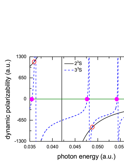
Figure 1: (Color online) Dynamic dipole polarizabilities (in a.u.) of helium for the photon energy $0.035\leq\omega\leq 0.06$ a.u. The solid black line denotes the dynamic polarizabilities for $2\,^{3}S$ state, and the dashed blue line represents the dynamic polarizabilities for $3\,^{3}S$ state. The crossing points denoted as solid magenta circle are the tune-out wavelengths, and the crossing points marked as blank red circle are the magic wavelengths. The vertical lines are the resonance transition positions, and the green line is a horizontal zero line.

Figure 2: (Color online) Dynamic dipole polarizabilities (in a.u.) of helium for the photon energy $0.06\leq\omega\leq 0.10$ a.u. The solid black line denotes the dynamic polarizabilities for $2\,^{3}S$ state, and the dashed blue line represents the dynamic polarizabilities for $2\,^{3}P(M=0)$ state. The crossing points denoted as solid magenta circle are the tune-out wavelengths, and the crossing points marked as blank red circle are the magic wavelengths. The vertical lines are the resonance transition positions, and the green line is a horizontal zero line.

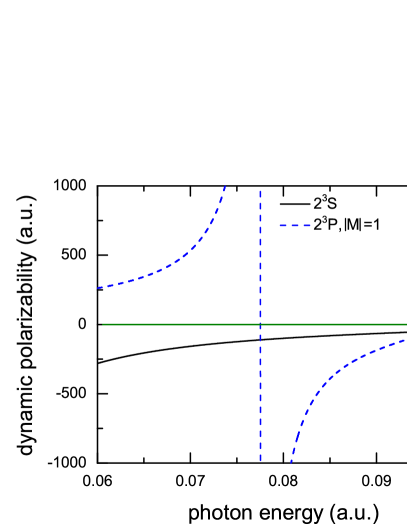
Figure 3: (Color online) Dynamic dipole polarizabilities (in a.u.) of helium for the photon energy $0.06\leq\omega\leq 0.10$ a.u. The solid black line denotes the dynamic polarizabilities for $2\,^{3}S$ state, and the dashed blue line represents the dynamic polarizabilities for $2\,^{3}P(|M|=1)$ state. The crossing points denoted as solid magenta circle are the tune-out wavelengths, and the crossing points marked as blank red circle are the magic wavelengths. The vertical lines are the resonance transition positions, and the green line is a horizontal zero line.

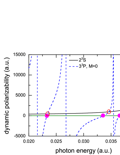
Figure 4: (Color online) Dynamic dipole polarizabilities (in a.u.) of helium for the photon energy $0.02\leq\omega\leq 0.04$ a.u. The solid black line denotes the dynamic polarizabilities for $2\,^{3}S$ state, and the dashed blue line represents the dynamic polarizabilities for $3\,^{3}P(M=0)$ state. The crossing points denoted as solid magenta circle are the tune-out wavelengths, and the crossing points marked as blank red circle are the magic wavelengths. The vertical lines are the resonance transition positions, and the green line is a horizontal zero line.

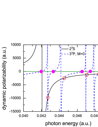
Figure 5: (Color online) Dynamic dipole polarizabilities (in a.u.) of helium for the photon energy $0.04\leq\omega\leq 0.05$ a.u. The solid black line denotes the dynamic polarizabilities for $2\,^{3}S$ state, and the dashed blue line represents the dynamic polarizabilities for $3\,^{3}P(M=0)$ state. The crossing points denoted as solid magenta circle are the tune-out wavelengths, and the crossing points marked as blank red circle are the magic wavelengths. The vertical lines are the resonance transition positions, and the green line is a horizontal zero line.

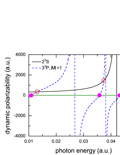
Figure 6: (Color online) Dynamic dipole polarizabilities (in a.u.) of helium for the photon energy $0.01\leq\omega\leq 0.05$ a.u. The solid black line denotes the dynamic polarizabilities for $2\,^{3}S$ state, and the dashed blue line represents the dynamic polarizabilities for $3\,^{3}P(|M|=1)$ state. The crossing points denoted as solid magenta circle are the tune-out wavelengths, and the crossing points marked as blank red circle are the magic wavelengths. The vertical lines are the resonance transition positions, and the green line is a horizontal zero line.

IV.4 Tune-Out Wavelengths

Table 8: Tune-out wavelengths ($\lambda_{t}$) for $2\,^{3}S$, $3\,^{3}S$, $2\,^{3}P$, and $3\,^{3}P$ states of helium. The second and third column are the tune-out wavelengths in atomic units and nanometer respectively. The numbers in parentheses give the computational uncertainties.

State	$\omega_{t}$(a.u.)	$\lambda_{t}$(nm)
$2\,^{3}S$	0.110 312 66(2)	413.038 28(3)
$3\,^{3}S$	0.035 488 102(2)	1283.905 03(4)
	0.047 681 245(3)	955.582 28(7)
	0.054 260 56(3)	839.714(2)
	0.058 1756(2)	783.204(2)
$2\,^{3}P(M=0)$	0.066 652 71(2)	683.5934(2)
	0.094 341 03(2)	482.9644(2)
	0.098 338 54(2)	463.3316(2)
$2\,^{3}P(M=\pm 1)$	0.097 382 82(2)	467.8788(2)
$3\,^{3}P(M=0)$	0.023 315 997(3)	1954.1670(3)
	0.033 637 088(2)	1354.5570(2)
	0.036 548 517(2)	1246.6539(3)
	0.042 005 02(2)	1084.712(2)
	0.043 390 63(3)	1050.074(2)
	0.046 5939(2)	977.883(2)
	0.047 4031(2)	961.189(3)
	0.049 4427(2)	921.539(4)
	0.049 9644(2)	911.917(4)
$3\,^{3}P(M=\pm 1)$	0.010 911 33(2)	4175.783(4)
	0.035 787 67(2)	1273.1580(2)
	0.043 149 27(2)	1055.9472(3)
	0.047 2945(1)	963.397(2)
	0.049 9054(1)	912.995(3)

Table 8 lists the values of tune-out wavelengths in the 400-4200 nm region, which marked as solid magenta circle in the Figs. 1- 6, For the metastable state of helium, Mitroy and Tang Mitroy and Tang (2013) have obtained the 413.02(9) nm tune-out wavelength by incorporating Hylleraas matrix elements for the transition to $2\,^{3}P$ and $3\,^{3}P$ manifolds and core-polarization model matrix elements for other transitions, and they predicted the tune-out wavelength around 413 nm can be used to test the QED effect. Recently, a experimental measurement of Ken Baldwin’s group report the tune-out wavelength being 413.0938(9Stat. )(20Syst.) nm Henson et al. (2015) and another theoretical calculation by Notermans et al Notermans et al. (2014) gives 414.197 nm tune-out wavelength by using available tables of level energies and Einstein A coefficients. Our tune-out wavelength of ab-initio calculation is 413.038 28(3) nm, which corroborates the value 413.02(9) nm of Mitroy and Tang Mitroy and Tang (2013). The difference between the theoretical calculations and the experimental measurement may caused by finite nuclear mass, relativistic and QED corrections, which calls for great efforts for theoretical calculation to improve the precision for QED test.

IV.5 Magic Wavelengths

Table 9: Magic wavelengths ($\lambda_{m}$) for $2\,^{3}S\to 3\,^{3}S$, $2\,^{3}S\to 2\,^{3}P(M=0,\pm 1)$ and $2\,^{3}S\to 3\,^{3}P(M=0,\pm 1)$ transitions of the He atom. The corresponding dynamic dipole polarizabilities at the magic wavelengths are given in the last column. The numbers in parentheses give the computational uncertainties.

Transition	$\omega_{m}(a.u.)$	$\lambda_{m}(nm)$	$\alpha_{1}(\omega_{m})(a.u.)$
$2\,^{3}S\to 3\,^{3}S$	0.036 004 592(2)	1265.48724(4)	1151.058(2)
	0.048 775 162(5)	934.1507(2)	$-$872.007(2)
	0.058 0244(2)	785.245(3)	$-$324.31(2)
$2\,^{3}S\to 2\,^{3}P(M=0)$	0.066 228 54(2)	687.9716(2)	$-$191.9157(2)
	0.093 2295(2)	488.7225(2)	$-$56.5068(2)
	0.098 0166(2)	464.8532(3)	$-$44.169 53(4)
$2\,^{3}S\to 2\,^{3}P(M=\pm 1)$	0.095 7473(2)	475.870 85(6)	$-$49.962 90(4)
$2\,^{3}S\to 3\,^{3}P(M=0)$	0.023 434 415(3)	1944.2923(3)	453.0297(2)
	0.034 618 094(3)	1316.1716(2)	955.639(2)
	0.037 202 6377(2)	1224.73446(2)	1410.365(2)
	0.042 734 44(3)	1066.197(2)	$-$9487(2)
	0.044 532 37(2)	1023.151(2)	$-$2511.07(3)
	0.047 069 3(2)	968.007(3)	$-$1196.32(3)
	0.048 478 5(2)	939.867(4)	$-$915.97(3)
	0.049 762 5(3)	915.616(5)	$-$750.19(3)
$2\,^{3}S\to 3\,^{3}P(M=\pm 1)$	0.013 031 86(2)	3496.304(3)	348.0648(2)
	0.037 297 86(2)	1221.607 75(2)	1436.592(2)
	0.044 421 15(2)	1025.713(2)	$-$2633.59(3)
	0.048 309 5(2)	943.156(4)	$-$942.89(2)

The magic wavelength is the wavelength at which the polarizability difference for a transition goes to zero, which means the first-order Stark shifts for the upper and lower levels of a transition are the same Ye et al. (1999); Safronova et al. (2013). Table 9 presents all the values of magic wavelengths in the 460-3500 nm region marked in blank red circle in the Figs. 1-6. The corresponding dynamic dipole polarizabilities at the magic wavelengths are also given in the last column. For the magic wavelength of 1066.197(2) nm, there exist two terms, which play major contribution of the dynamic dipole polarizabilities for the $2\,^{3}S$ and $3\,^{3}P(M=0)$ states respectively. Table 10 lists some contributions from different intermediate states for the $2\,^{3}S\to 3\,^{3}P(M=0)$ transition in detail at the magic wavelength of 1066.197(2) nm. We can see that the contribution from $2\,^{3}P$ state to the polairzability of $2\,^{3}S$ is about 99.87%, and the contribution from $6\,^{3}S$ state to the polairzability of $3\,^{3}P(M=0)$ is about 98.87%. According to the definition of magic wavelength $\alpha_{2\,^{3}S}(\omega_{m})=\alpha_{3\,^{3}P}(\omega_{m})$, we have the expanded form,

$$\frac{f_{2\,^{3}S\to 2\,^{3}P}}{\Delta E_{2\,^{3}S\to 2\,^{3}P}^{2}-\omega_{m}^{2}}+\alpha_{2\,^{3}S}(Remainder;\omega_{m}) = \frac{3f_{3\,^{3}P\to 6\,^{3}S}}{\Delta E_{3\,^{3}P\to 6\,^{3}S}^{2}-\omega_{m}^{2}}+\alpha_{3\,^{3}P}(Remainder;\omega_{m})$$

where the second term in the left of Eq. (IV.5) is all the contributions from other $n\,^{3}P$ states to the dynamic dipole polarizability of $2\,^{3}S$ state, and the second term in the right of Eq. (IV.5) is all the contributions from other $n\,^{3}S$, $n\,^{3}D$, and $n\,^{3}P^{e}$ states to the dynamic dipole polarizability of $3\,^{3}P(M=0)$ state. If all the remainder terms are neglected, then the ratios of oscillator strengths and reduced matrix elements are written as

$$\frac{f_{2\,^{3}S\to 2\,^{3}P}}{f_{3\,^{3}P\to 6\,^{3}S}} = \frac{3(\Delta E_{2\,^{3}S\to 2\,^{3}P}^{2}-\omega_{m}^{2})}{\Delta E_{3\,^{3}P\to 6\,^{3}S}^{2}-\omega_{m}^{2}}$$ (42)

$$\frac{M_{2\,^{3}S\to 2\,^{3}P}}{M_{3\,^{3}P\to 6\,^{3}S}} = \frac{|\langle 2\,^{3}S\|\sum\limits_{i=1,2}r_{i}C^{(1)}(\hat{r}_{i})\|2\,^{3}P\rangle|}{|\langle 3\,^{3}P\|\sum\limits_{i=1,2}r_{i}C^{(1)}(\hat{r}_{i})\|6\,^{3}S\rangle|}=\sqrt{\frac{\Delta E_{3\,^{3}P\to 6\,^{3}S}(\Delta E_{2\,^{3}S\to 2\,^{3}P}^{2}-\omega_{m}^{2})}{\Delta E_{2\,^{3}S\to 2\,^{3}P}(\Delta E_{3\,^{3}P\to 6\,^{3}S}^{2}-\omega_{m}^{2})}}$$ (43)

Combined present energy difference and the magic wavelength 1066.197(2) nm, the ratios of the oscillator strengths and the reduced matrix elements are determined and listed in Table 11. Present¹ are the values of our ab-initio calculation, and Present² are derived by substituting our theoretical energies and the magic wavelength of 1066.197(2) nm into the Eqs.(42) and (43). Compared with the explicitly correlated results of Ref. Cann and Thakkar (1992), we believe our values of Present¹ are reliable, since present oscillator strengths for $2\,^{3}S\to 2\,^{3}P$ and $3\,^{3}P\to 6\,^{3}S$ transitions are much more accurate than the values of Ref. Cann and Thakkar (1992) by at least one order of magnitude. In order to test the accuracy of the values derived from Eqs.(42) and (43), we can compare the results between Present¹ and Present². It’s clearly seen that the derived values 64.6653 and 4.677847 from the Eqs.(42) and (43) are in good agreement with our ab-initio values 65.48(2) and 4.7073(3) at the level of 1.3% and 0.7% accuracy respectively. If increasing the number of B-spline basis sets, and also considered the contribution of the remainder term, then improvement of the accuracy for the transition matrix elements ratio $(M_{2\,^{3}S\to 2\,^{3}P})/(M_{3\,^{3}P\to 6\,^{3}S})$ up to 0.5% is achievable.

As we known that, present experimental technique is very difficult to measure matrix elements accurately, only 1% accuracy for one or two of the lowest transitions have been reported Gomez et al. (2004); Bouloufa et al. (2009). Recently, Herold et al. present a method for accurate determination of $5s-6p$ matrix elements in rubidium by measurements of the ac Stark shift around tune-out wavelength Herold et al. (2012). In our calculation, the particular magic wavelength around 1066 nm can be used for experiment measurement to determine the atomic transition matrix elements involved highly excited states for helium.

Table 10: Contributions from some of intermediate states to the dynamic dipole polarizability of $2\,^{3}S$ and $3\,^{3}P(M=0)$ states at the magic wavelengths 1066.197(2) nm.

$\omega(a.u.)$	0.042 734 44(3)
$\lambda(nm)$	1066.197(2)
Intermediate states	$2\,^{3}S$
$2\,^{3}P$	$-$9499.066
$3\,^{3}P$	5.418
$4\,^{3}P$	1.386
Others	5.234
Total	$-$9487.028
Intermediate states	$3\,^{3}P(M=0)$
$3\,^{3}S$	519.840
$4\,^{3}S$	$-$320.109
$5\,^{3}S$	$-$118.888
$6\,^{3}S$	$-$9379.600
$3\,^{3}D$	$-$73.9017
$4\,^{3}D$	$-$517.059
$5\,^{3}D$	$-$395.758
$6\,^{3}D$	506.415
Others	292.0327
Total	$-$9487.028

Table 11: Comparison of the ratios for the oscillator strengths $(f_{2\,^{3}S\to 2\,^{3}P})/(f_{3\,^{3}P\to 6\,^{3}S})$ and the reduced matrix elements $(M_{2\,^{3}S\to 2\,^{3}P})/(M_{3\,^{3}P\to 6\,^{3}S})$. Present¹ are the value of our ab-initio calculation, and Present² are derived by substituting our theoretical energies and the magic wavelength of 1066.197(2) nm into the Eqs.(42) and (43). The numbers in parentheses give the computational uncertainties.

	$(f_{2\,^{3}S\to 2\,^{3}P})/(f_{3\,^{3}P\to 6\,^{3}S})$	$(M_{2\,^{3}S\to 2\,^{3}P})/(M_{3\,^{3}P\to 6\,^{3}S})$
Present1	65.48(2)	4.7073(3)
Present2	64.6653	4.677847
Ref. Cann and Thakkar (1992)	65.5308	4.789739

V conclusions

The calculations of the energies and the main oscillator strengths for the four triplet states ($2\,^{3}S$, $3\,^{3}S$, $2\,^{3}P$, and $3\,^{3}P$) in the length, velocity and acceleration gauges are carried out by the configuration interaction based on the B-spline functions. Also the accurate dynamic dipole polarizabilities for the four lowest triplet states are obtained. Ours static dipole polarizabilities in the length and velocity gauges have 5-6 significant digits, which are in excellent agreement with the variational Hylleraas calculations. Present work lays solid foundation for the further to calculate the relativistic and QED effects on the dynamic polarizabilities of helium.

In particular, the tune-out wavelengths for the four triplet states and magic wavelengths for the three transitions of $2\,^{3}S\to 3\,^{3}S$, $2\,^{3}S\to 2\,^{3}P$, and $2\,^{3}S\to 3\,^{3}P$ are determined with high precision. Our tune-out wavelength 413.038 28(3) nm of the metastable state validate the value of Mitroy and Tang Mitroy and Tang (2013). And the magic wavelength around 1066 nm for $2\,^{3}S\to 3\,^{3}P$ transition is proposed for experimental measurement to determine the ratio of the transition matrix elements ($2\,^{3}S\to 2\,^{3}P)/(3\,^{3}P\to 6\,^{3}S$), this is a unique way to obtain accurate transition matrix element involved highly excited states. Also we expected that other tune-out wavelengths and magic wavelengths can provide theoretical reference for the precision-measurement experiment design in the future.