Triple Stars Observed by Kepler

Abstract

The Kepler mission has provided high quality light curves for more than 2000 eclipsing binaries. Tertiary companions to these binaries can be detected if they transit one or both stars in the binary or if they perturb the binary enough to cause deviations in the observed times of the primary and secondary eclipses (in a few cases both effects are observed in the same eclipsing binary). From the study of eclipse timing variations, it is estimated that 15 to 20% of the Kepler eclipsing binaries have close-in tertiary companions. I will give an overview of recent results and discuss some specific systems of interest.

¹Department of Astronomy, San Diego State University, San Diego, California, United States; jorosz@mail.sdsu.edu

1 Introduction

In an isolated, detached eclipsing binary (EB), the eclipses should be strictly periodic, with a constant interval of time between successive eclipses. In these cases, the times of eclipse are described by a simple linear ephemeris:

$$T_{\rm min}(E)=T_{0}+P_{\rm bin}E$$ (1)

where $P_{\rm bin}$ is the binary orbital period and $E$ is the cycle number. The residuals derived from a fit to a linear ephemeris form an “Observed minus Computed” or O-C diagram. If one measures eclipse times (ETs) for both primary and secondary eclipses, then both types of events may be put on a common system by means of a phase offset $\delta$ that is applied to the cycle numbers of the secondary eclipses. A single period can then be fit to all of the ETs. We will refer to the resulting O-C diagram a “Common Period O-C” or CPOC diagram.

There are a number of situations where the intervals between successive eclipses are not constant, thereby leading to eclipse timing variations (ETVs). The points in the O-C or CPOC diagrams will no longer be scattered about the horizontal axis, and a model that goes beyond a simple linear ephemeris will be needed. We briefly discuss mechanisms for ETVs that apply to stars that are well within their respective Roche lobes, where mass transfer and mass loss can be neglected.

If the EB is part of a triple system, then the eclipses will either be early or late owing to light travel time (LTT) changes as the EB moves about the center of mass of the triple system. In these cases, the ETs are no longer described by a simple linear ephemeris (e.g. Irwin 1952):

$$T_{\rm min}(E)=T_{0}+P_{\rm bin}E+K\left[{1-e_{3}^{2}\over 1+e_{3}\cos\nu_{3}}\sin(\nu_{3}+\omega_{3})+e_{3}\sin\omega_{3}\right],$$ (2)

where $e_{3}$ is the eccentricity and $\omega_{3}$ is the longitude of periastron of the tertiary orbit, $\nu_{3}$ is the true anomaly in that orbit, and where the semi-amplitude $K$ is given by

$$K={a_{12}\sin i^{3}\over c},$$ (3)

where $a_{12}$ is the semimajor axis of the EB orbit about the third star, $i_{3}$ is the inclination to the observer’s line-of-sight, and where $c$ is the speed of light. The minimum mass of the third body can be computed in a way that is similar to the well-known result that can be derived from a radial velocity curve:

$$f(M_{3})={M^{3}_{3}\sin^{3}i_{3}\over(M_{1}+M_{2}+M_{3})^{2}}={4\pi^{2}(a_{12}\sin i_{3})^{3}\over GP^{2}_{3}}$$ (4)

where $M_{1}$ and $M_{2}$ are the masses of the stars in the EB, $M_{3}$ is the tertiary mass, and $G$ is the constant of gravitation. Many close EBs are found to have third components based on LTT studies (e.g. Tokovinin et al. 2006).

If the third star is in a relatively close orbit with the EB, then the changing proximity of the third body can affect the orbital period of the inner binary. Borkovits et al. (2003) presented an analytic study of the ETVs caused by an exterior, perturbing object on a large, eccentric orbit. The signals one sees in the O-C diagrams can be quite complex, depending on the eccentricities of the EB and outer orbit, and on the mutual inclinations of the orbits.

Before the launch of Kepler, EBs where dynamical effects dominate the ETVs were comparatively rare. One example is IU Aurigae (Özdemir et al. 2003), which is a massive binary ($M_{1}=21.4\,M_{\odot}$ and $M_{2}=14.5\,M_{\odot}$) with an orbital period of 1.8 days. There is a third body with a period of 293 days which causes precession of the inner binary on a time-scale of $\approx 335$ years. If the ETVs are taken to be from LTT effects alone, then the minimum mass of the third body is about $15\,M_{\odot}$, which is much too massive, given the amount of third light measured from spectroscopy and from the light curve solutions. Hence Özdemir et al. (2003) argue that a large part of the signal seen in the O-C diagram is due to dynamical effects. Another example is SS Lac, which was known to be a deeply eclipsing EB around the year 1900, but then stopped eclipsing around the year 1950, presumably due to the influence of a third body. This outer body with a period of 697 days was detected spectroscopically by Torres & Stefanik (2000). In a subsequent paper, Torres (2001) modeled the depth changes of the eclipses and found a precession period of about 600 years. More recently, Graczyk et al. (2011) found 17 EBs in the LMC via the OGLE survey where the eclipse depths changed. In two cases the eclipses disappeared altogether.

The line of apsides of an eccentric binary can rotate due to the effects of General Relativity. The ratio of the orbital period of the binary to the rotation period $U_{\rm GR}$ of the line of apsides is given by

$${P_{\rm bin}\over U_{\rm GR}}=6.35\times 10^{-6}\left({M_{1}+M_{2}\over a(1-e^{2})}\right)$$ (5)

where $M_{1}$ and $M_{2}$ are the masses of each star in solar masses, and $a$ is the semimajor axis of the relative orbit in solar radii (Kopal 1978). In addition, tidal distortions can cause the line of apsides of an eccentric binary to rotate with a period $U_{\rm tide}$ given by

$${P_{\rm bin}\over U_{\rm tide}}=c_{21}k_{21}+c_{22}k_{22}$$ (6)

where $k_{12}$ and $k_{22}$ are the so-called internal structure constants of the stars, and where the coefficients $c_{21}$ and $c_{22}$ are given by

$$c_{21} = \left[\left({\omega_{1}\over\omega_{K}}\right)^{2}\left(1+{M_{2}\over M_{1}}\right)f(e)+{15M_{2}\over M_{1}}g(e)\right]\left({R_{1}\over a}\right)^{5}$$

$$c_{22} = \left[\left({\omega_{2}\over\omega_{K}}\right)^{2}\left(1+{M_{1}\over M_{2}}\right)f(e)+{15M_{1}\over M_{2}}g(e)\right]\left({R_{2}\over a}\right)^{5}.$$ (7)

In the above equations, ($\omega_{1}/\omega_{K}$) and ($\omega_{2}/\omega_{K}$) are the ratios between the actual angular rotational velocity of the stars and the rotational velocity corresponding to synchronization with the average orbital velocity. The functions $f(e)$ and $g(e)$ are given by

$$f(e) = {1\over(1-e^{2})^{2}}$$

$$g(e) = {(8+12e^{2}+e^{4})f(e)^{2.5}\over 8}$$ (8)

(Claret & Giménez 1993). Note that the expected apsidal period depends on the fifth power of the fractional radii of the stars, and that for EBs with periods more than about 15 to 20 days the apsidal period will usually be factors of several million or more times the binary period, assuming the EBs contain solar-type main sequence stars.

Since the phase difference between the primary and secondary eclipses changes with time, “apsidal motion” due to General Relativity or to tides will give rise to ETVs, where the O-C curves of the primary and secondary roughly resemble sine curves that are 180 degrees out of phase. Unfortunately there are no simple close-form expressions to model the signal seen in the O-C diagram of an eccentric EB undergoing apsidal motion. Giménez & Garcia-Pelayo (1983) give a power series expression up to the fifth power of the eccentricity that contains roughly 50 terms. Lacy (1992) presented an exact solution based on an iterative solution of the transcendental equations involved.

2 The Kepler EB Sample

The Kepler mission (Borucki et al. 2010) observed over 2000 EBs with a duty cycle on the order of 90% or greater, and good photometric precision (Prša et al. 2011, Slawson et al. 2011). These data give us the unique opportunity to measure precise ETs and detect deviations from a linear ephemeris. Previously, Gies et al. (2012) measured ETs for 41 Kepler EBs using data through Q9 ($\approx 2$ year baseline). They found no evidence for short-period companions with periods smaller than $\approx 700$ days in the sample, but did find evidence for long-term trends in 14 systems. Rappaport et al. (2013) did a much more thorough survey where they measured ETs for 2175 Kepler EBs using data through Q13 ($\approx 3$ year baseline). They identified 39 candidate triple systems. Conroy et al. (2014) presented a catalog of ETs for 1279 close binaries (e.g. the overcontact and ellipsoidal EBs with periods generally smaller than 1 day) in the Kepler sample. There were 236 systems where the ETVs were compatible with the presence of a third body.

We give an update on our own program to measure accurate ETs for the Kepler EBs with periods longer than about 1 day. We have developed a suite of algorithms and codes (collectively called “TEMPUS”) to automatically measure times of mid eclipse for detached Kepler EBs. TEMPUS was developed on and runs in the Matlab environment. An earlier version of the software was described in Steffen et al. (2011). TEMPUS has evolved since then, so a new overview is presented here.

TEMPUS is a computational system for measuring ETs from the Kepler SAP light curves. Briefly, a model eclipse profile constructed from the data is used to find individual ETs. Because the ETs may not be described by a simple linear ephemeris, an iterative method is used. The iteration begins with an initial set of ET values, usually computed from a linear ephemeris. The eclipses in the data are found and locally detrended using a cubic spline. The detrending algorithm requires that each eclipse event has well-defined “shoulders” so that the first and fourth contact points can be identified. When such shoulders are present, we have found the local detrending works well in most cases. Once the individual eclipse events are locally detrended, they are folded to produce an eclipse profile. A piecewise cubic Hermite spline (PCHS) model is then fit to this profile. During this process, nearby data are tested for gaps and other problems that would compromise the determination of that ET value. Those ETs that exhibit such problems are eliminated from further consideration. The PCHS is then used to improve the ET estimates, and those, in turn, provide an improved eclipse profile constructed from the local detrending and folding. This iteration is run three times. At this point the ET estimates are significantly improved and the eclipses with compromised data have been eliminated. However, there remains a chance that a good eclipse may have been eliminated as the ET estimates were being adjusted. Therefore, using the latest ET estimates this iterative process is restarted with any missing ET estimates being approximated by nearby ones. After three additional iterations, the so-called Pipeline has produced very good ET estimates and a very good PCHS model of the eclipse profile.

The final step in the process is to compute an unbinned PCHS model that when binned to the Kepler Long Cadence exposure time (29.4244 minutes) will best represent the eclipse profile made from the detrended and folded data. As an initial approximation, the PCHS resulting from the six iterations is used. It is binned for each point in the latest locally-detrended and folded data and used to improve the ET estimates. These ET estimates again determined a revised local detrending and folding of the data with a best, unbinned PCHS model being computed and, in turn determining a further, but very minor, revision in the ET estimates. The last iteration of this process occurs with the final result being a PCHS model that, when binned, optimally describes the eclipse profile produced from the locally detrended and folded data, which are determined by the latest ET estimates.

During this process, ETs that are outliers to the individual model fits are eliminated from defining further models but remain as values to be estimated. The error estimates for each ET value use the standard approach of sliding the model, in time, across the ET estimate and noting when the $\chi^{2}$ curve rises above the $1\sigma$ threshold.

Producing a fully automated process to measure ETs for Kepler EBs is a difficult task owing to the wide variety of light curve morphologies (e.g. see Prša et al. 2011 and Slawson et al. 2011): Many binaries are spotted, many of them have pulsations, many binaries have deep eclipses, and others are severely diluted. In order to have confidence in the results, the TEMPUS pipeline produces many diagnostic plots such as plots of the individual O-C and CPOC diagrams, plots of the observed and model eclipse profiles, power spectra of the ETVs, and plots of a small subset of the “raw” light curve. These plots were inspected by eye and interesting systems were selected.

3 Results

We used all of the available long cadence data through Q16 as input to TEMPUS. Our initial sample consisted of the 1322 binaries from the catalog of Slawson et al. (2011) classified as either detached or semidetatched, supplemented with some additional EBs that were discovered since that publication. As the orbital period gets shorter and shorter, reflection effects and tidal distortion tend to make the out-of-eclipse regions increasingly curved. Since our technique requires well-defined eclipse shoulders to work, we placed a cutoff at orbital periods shorter than 0.9 days. This cutoff removed a few hundred binaries from the sample, leaving 1258. These binaries were fed into TEMPUS to measure the ETs, and 1249 systems had their primary ETs measured successfully. The cases that failed either lacked well-defined shoulders, or had very low signal-to-noise eclipses. Eccentric binaries can have primary eclipses and no secondary eclipses, so the sample of binaries with measurable secondary eclipses is somewhat smaller. In the end, a total of 764 systems had both primary and secondary ETs measured successfully. The typical uncertainties on the ETs range from a few seconds to several minutes for the noisy cases.

The diagnostic plots from TEMPUS were inspected and obvious spurious cases were removed. Particular attention was paid to the plots showing the final eclipse profile and final PCHS model. Based on the quality of the fits to the eclipse profiles, 335 EBs were removed from the sample, leaving 914 systems.

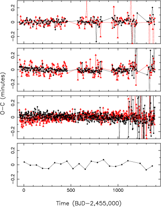
Figure 1.: Left: Example CPOC diagrams where the rms scatter in the ETVs is smaller than $\approx 10$ sec. The black points show the primary ETVs and the red points show the secondary ETVs. From top to bottom, the systems are KIC 9913481, KIC 10156064, KIC 10191056, and KIC 12356914. Right: The distribution of the rms of the primary ETVs in minutes. Most of the systems have reasonably small scatter, although the tail of the distribution extends to much higher rms values.

Finally, for each binary, the O-C diagrams for the primary eclipses and secondary eclipses (if present) were made. In cases where both primary and secondary eclipses were present, an iterative procedure was used to produce a CPOC diagram. These plots were visually inspected, and interesting cases were selected. We give below an overview of these results.

3.1 EBs With Small ETVs

One simple statistic to compute is the rms of the primary ETVs. A large rms in the ETVs may indicate the presence of a nearby third body, although one needs to verify this on a case-by-case basis (for example, star spots can induce spurious ETV signals as discussed below). Likewise, a small rms in the ETVs might be used to place limits on the lack of a third body, although, again, one needs to verify each case individually. There may be cases where long-term trends are evident in spite of the small rms, or cases where the primary and secondary ETV signals diverge in the CPOC. Figure 1 shows four examples where the primary and secondary rms values are smaller than about 10 seconds. Figure 1 also shows the distribution of rms values for the primary ETVs. The histogram peaks around 10 seconds. A total of 502 systems have rms values smaller than 30 seconds and 741 systems have rms values of smaller than one minute.

Figure 2.: Left: Eclipses of a star spot in Kepler-47. A dark spot on the primary star rotates in and out of view, leading to the variable flux in the out-of-eclipse regions as shown at the bottom. This star spot was partially eclipsed by the secondary star during five consecutive primary eclipses. When the eclipse is modeled with a symmetric function, a hump appears in the residuals. As the spot moves on the primary, the phase of the hump in the residuals changes. Right: The O-C values of the primary eclipses in Kepler-47 vs the local light curve slope. The eclipses are systematically late when the out-of-eclipse flux slopes downward during a primary eclipse (this occurs when the dark spot is rotating into view), and systematically early when the out-of-eclipse flux slopes upward during a primary eclipse (this occurs when the dark spot is rotating out of view). Figures from Orosz et al. (2012).

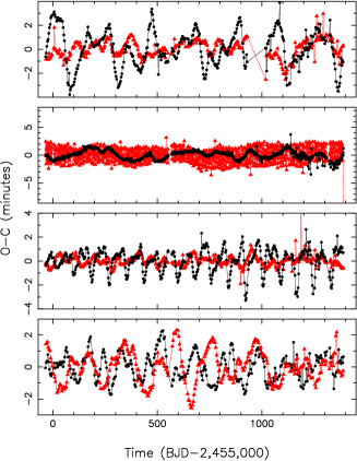
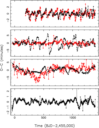
Figure 3.: Example CPOC diagrams where the ETVs are affected by star spots, giving rise to “random” walk signals (the color scheme is the same as the left panel in Figure 1). From top to bottom and left to right, the systems are KIC 4908495, KIC 6697716, KIC 6706287, KIC 6863840, KIC 7374746, KIC 9005854, KIC 10346522, and KIC 12418816.

3.2 EBs with Star Spots

In an EB with immaculate stars, the eclipse profiles should be smooth and symmetric in time for EBs with small eccentricities. If a star spot (either dark or bright) appears on the star that is being eclipsed, then the eclipse profile will appear distorted. The distortion can be relatively large in cases where the body in front is much smaller than the body that is being eclipsed. If one is using a symmetric model profile to find the time of minimum light, there will be a hump in the residuals of the profile fit and the resulting time will have a systematic error. The primary eclipses in Kepler-47 illustrate this quite nicely as shown in Figure 2 (taken from Orosz et al. 2012, see also Sanchis-Ojeda et al. 2012). One or more dark spots on the primary rotate into and out of view, leading to a modulation in the out-of-eclipse regions of the light curve. When the light curve has a downward slope near primary eclipse, a dark spot is rotating into view, and when the light curve has an upward slope near primary eclipse, there is a dark spot rotating out of view. Figure 2 shows a sequence of five primary eclipses where the local slope of the light curve goes from being positive to negative during the eclipse. The spot is in a different place on the primary star during successive primary eclipses, and as a result the phase of the hump in the residuals changes. For Kepler-47 and many other EBs, there is a correlation between the ETV of an eclipse time and the local slope of the light curve during that eclipse (Sanchis-Ojeda et al. 2012), as shown in Figure 2. The presence of this correlation in Kepler-47 is a good indication that the signal seen in the ETVs of the primary star is spurious, as the ETVs, corrected using this correlation, show no signal (Orosz et al. 2012).

Because star spots seem to come and go, an EB with spots may exhibit a “random walk” signal in the CPOC diagram. Such a signal could have systematic deviations much larger than the nominal uncertainties in the ETs, but will not remain coherent over the long term. During the visual inspections of the CPOC diagrams, 117 EBs with random walk signals were identified, and Figure 3 shows eight example cases.

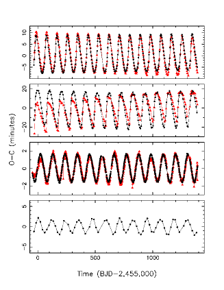
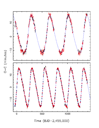
Figure 4.: Left: Example CPOC diagrams for systems with obvious periodicities, where the color scheme is the same as in Figure 1. From top to bottom, the EBs are KIC 6545018 ($P_{\rm bin}=3.99$ d, $P_{\rm out}=90.4$ d), KIC 9714358 ($P_{\rm bin}=6.47$ d, $P_{\rm out}=103.8$ d), KIC 9451096 ($P_{\rm bin}=1.25$ d, $P_{\rm out}=106.9$ d), and KIC 5095269 ($P_{\rm bin}=18.6$ d, $P_{\rm out}=117.9$ d). Right: Two EBs with periodic signals in their CPOC diagrams where LTT model fits (blue lines) yield very high tertiary masses. From top to bottom, the EBs are KIC 4940201 ($P_{\rm bin}=8.82$ d, $P_{\rm out}=363.7$ d, $f(M)=4.53\,M_{\odot}$), and KIC 5384802 ($P_{\rm bin}=6.08$ d, $P_{\rm out}=255.2$ d, $f(M)=13.92\,M_{\odot}$).

3.3 EBs with Obvious Periodicities in the CPOC

During our visual inspections of the O-C and CPOC diagrams, we identified 55 EBs with obvious periodicities in the primary ETVs, including 7 with periods smaller than 200 days. Figure 4 shows O-C and CPOC diagrams for the four shortest-period ones, with ETV periods of 90.4, 103.8, 106.9, and 117.9 days. These periods almost certainly indicate the period of the third body. A literature search found mention of three EBs that were known before the launch of Kepler with third bodies having periods smaller than 200 days.

The EBs where the primary and secondary ETVs are periodic and track each other in the CPOC diagram can be modeled with an LTT orbit (Equation 2) and the minimum mass (hereafter the “mass function”) of the third body can be computed using Equation 4. A few EBs have implausibly large mass functions, and Figure 4 shows the CPOC diagrams of the two EBs with the largest mass functions ($4.53\,M_{\odot}$ and $13.92\,M_{\odot}$). As shown by Borkovits et al. (2003) and Rappaport et al. (2013), dynamical effects can sometimes produce ETV signals that can mimic ETVs due to pure LTT effects. Thus one should use extreme caution when modeling ETV signals with a simple LTT model.

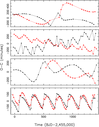
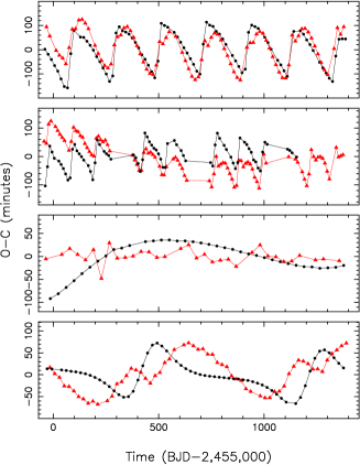
Figure 5.: Example CPOC systems where the range in the ETVs is too large to be caused by LTT effects only (the color scheme is the same as in Figure 1). From top to bottom and left to right, the systems are KIC 5255552 ($\Delta_{O-C}=13.3$ hr), KIC 7668648 ($\Delta_{O-C}=8.7$ hr), KIC 5653126 ($\Delta_{O-C}=6.7$ hr), KIC 7955301 ($\Delta_{O-C}=3.6$ hr), KIC 7955301 ($\Delta_{O-C}=3.6$ hr), KIC 5771589 ($\Delta_{O-C}=3.5$ hr), KIC 5003117 ($\Delta_{O-C}=2.5$ hr), and KIC 8210721 ($\Delta_{O-C}=2.5$ hr).

3.4 EBs with Large ETVs, Changing Eclipse Depths, and Tertiary Eclipses

We have found about a dozen systems where the range on the ETVs alone rules out simple LTT effects as the sole cause of the variations. Figure 5 shows the eight systems with the largest ETV spreads. KIC 5255552 has a spread of about 13.2 hours, which would require a displacement of the binary by about 100 AU if the ETVs were due entirely to LTT effects. We conclude the cause of these ETV signals is largely dynamical.

There are at least 16 EBs that show significant changes in the eclipse depths due to dynamical interactions. Figure 6 shows the light curves and CPOC diagrams for eight of these depth-changing systems. In all cases, there are significant ETVs, which is another indication that the depth changes are due to dynamical interactions.

Although hundreds of EBs with a tertiary companion were known prior to the launch of Kepler, none were observed to have eclipse events due to the third star. KOI-126 was the first system with tertiary events identified in the Kepler data (Carter et al. 2011). We have identified 24 EBs that show additional eclipse events due to a third body, including the circumbinary planet systems (there are a few other cases where there appear to be two unrelated EBs on the same Kepler pixel). Figure 7 shows eight examples. The presence of these additional eclipse events provides very strong constraints on the parameters of the system. Modeling these light curves can be difficult, but one is then rewarded with extremely precise parameters (e.g. Carter et al. 2011; Doyle et al. 2011).

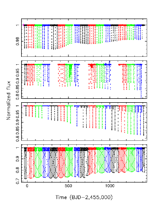
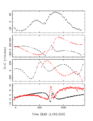
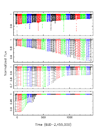
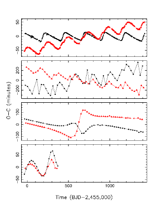
Figure 6.: Example EBs where the depths of the eclipses have changed due to the influence of a third body. The normalized Kepler light curves are shown on the left, where different colors denote the Kepler Quarter (black for Q1, Q5, Q9, Q13, and Q17; red for Q2, Q6, Q10, and Q14; green for Q3, Q7, Q11, and Q15; and blue for Q4, Q8, Q12 and Q16). The corresponding CPOC diagrams are shown on the right with the same color scheme as in Figure 1. From top to bottom, the systems are KIC 4769799, KIC 5255552 (this system fell on the bad CCD module during Q5, Q9, Q13, and Q17), KIC 5653126 (note the appearance of the secondary eclipses starting in Q8), KIC 5731312, KIC 7289157 (note the additional events due to the third body), KIC 7668648, KIC 7670617, and KIC 10319590.

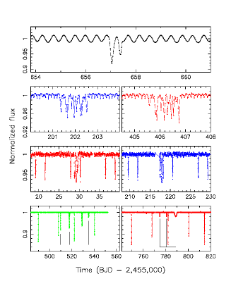
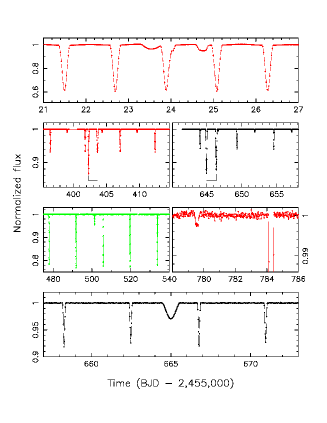
Figure 7.: Some EBs that show tertiary events due to a third star. The color scheme for the light curves is the same as in Figure 6. From left to right and top to bottom, the EBs are KIC 2835289, KIC 2856960, KIC 4150611, KIC 5255552, KIC 6543674, KIC 7289157, KIC 7668648, and KIC 7670485.

3.5 EBs with Long-Term Trends or Diverging CPOCs

We found 140 EBs with long-term trends in the ETVs. These trends presumably represent a small part of a signal with a periodicity that is much longer than our $\approx 4$ year baseline. Figure 8 shows four examples. The ETVs for the primary usually, but not always, track the ETVs for the secondary in the CPOC diagram.

We also found 107 EBs where the primary ETVs and secondary ETVs have roughly linear trends with opposite slopes in the CPOC diagram. The ETVs with opposite slopes occur when only a small part of an apsidal period is observed. Unlike the cases with large ETVs or periodic ETVs, having opposite linear trends in the CPOC diagram does not necessarily indicate the presence of the third body. As noted earlier, apsidal motion can be caused by tidal effects and/or General Relativity. While there are good analytic approximations for the rate of the apsidal advance, one needs to know the masses to apply the expression for GR precession and the masses and fractional radii to apply the expression for the tidal apsidal precession. If one assumes masses near a solar mass for each star, then detailed models of the light curves can give good estimates of the eccentricity of the binary and the fractional radii, making the expected rates of apsidal motion due to tides and GR computable. We are in the process of modeling the light curves to determine what fraction of the EBs where the opposite trends in the CPOC diagram could be explained by GR, tidal apsidal motion, or a combination of the two. In the absence of detailed light curve modeling, one can make a quick estimate by considering only the systems with orbital periods longer than about 20 days, as the expected apsidal rates for GR and tides fall off rapidly with increasing period, leaving the influence of a third body as the probable cause of the opposite trends in the CPOC diagram.

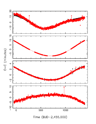
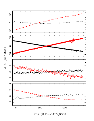
Figure 8.: Left: Some EBs that show long-term trends in their ETVs. From top to bottom, the EBs are KIC 4732015, KIC 5513861, KIC 8429450, and KIC 8553788. Right: Some EBs that have rougly linear trends with opposite slopes in the CPOC diagram. From top to bottom, the EBs are KIC 3247294, KIC 4544587, KIC 5955321, and KIC 8553907.

On a related note, when the primary ETVs and the secondary ETVs show opposite trends in the CPOC diagram, this means that one would get two different periods when fitting the primary ETs and the secondary ETs separately. We find 184 EBs where the primary eclipse period differs from the secondary eclipse period by more than $3\sigma$. Not all of these cases have roughly linear signals in the CPOC (for example KID 7289157 in Figure 6), and therefore the number of systems found by this test exceeds the 107 systems found above. There are 136 EBs out of the 184 with orbital periods 20 days or shorter, so in many of these cases the period differences could be due to GR and/or tides. For example, the primary and secondary periods of KIC 4344587 differ by $\approx 901\sigma$ (the mean period is about 2.19 days). Gies et al. (2012) showed that this period difference could be plausibly explained by tidal apsidal motion, as both stars in this short-period eccentric binary have relatively large fractional radii. On the other hand, we have 48 systems with significant period differences where the mean orbital period is longer than 20 days, and the influence of a third body will almost certainly be needed to explain the period differences in these cases.

3.6 A Brief Note on the Occurrence Rate of Close Triples

In their limited survey of 41 EBs, Gies et al. (2012) found 14 EBs with long-term trends, which represents 34% of the sample. They argued that “this finding is consistent with the presence of tertiary companions among a significant fraction of the targets, especially if many have orbits measured in decades”. In their more extensive survey, Rappaport et al. (2013) found 39 candidate triple systems and after accounting for the types of systems to which their search was sensitive, concluded that at least 20% of all close binaries have third body companions. Conroy et al. (2014) found 236 candidate triple systems out of 1279 searched, for a rate of about 18%.

Although this work is ongoing, we can make some preliminary estimates of the occurrence rate of triples in our sample. The O-C diagrams for the primary eclipses were visually inspected, and the ETV signal was assigned one of 6 classes: 1 for flat signal, 2 for an obviously periodic signal, 3 for a trend that is concave upwards, 4 for a trend that is concave downward, 5 for a “wiggle” (see KIC 5731312 in Figure 6), and 6 for a random walk due to star spots. The ETV signals for categories 2, 3, 4, and 5 will most likely be due to third bodies. There were 203 systems with one of these four designations out of the 1249 systems measured, which is about 16%. If we use the 914 EBs with acceptable profile fits as the sample size, then the fraction is 22%. In addition, the CPOC diagrams for all systems with both measured primary and secondary eclipses were inspected, and the ones where the primary ETV signal diverged from the secondary ETV signal were flagged. There were 112 such cases. In total there are 285 unique systems from both lists, which is 22.8% of the sample using a sample size of 1249 or 31% using a sample size of 914. As explained earlier, some of the EBs with roughly linear trends with opposite slopes in the CPOC diagram may not have third bodies (e.g. apsidal precession due to GR or tides may be sufficient to explain the ETVs). Thus, the 22.8% or 31% figures are upper limits. Nevertheless, we can say that based on our results so far, we can corroborate the results of Rappaport et al. (2013) who concluded that the occurrence rate of triples is on the order of 20%.

3.7 Models of Individual Systems

We have begun a program to systematically model the light and velocity curves of several EBs with large ETVs and/or tertiary eclipse events. The usual binary light curve synthesis codes are not adequate as the positions of the stars are not described by simple Keplerian orbits. We modified the ELC code (Orosz & Hauschildt 2000) to include a dynamical integrator that solves the Newtonian equations of motion to give the positions of the stars at any given time. Given the positions of the stars, their radii, their relative flux contributions, and their limb darkening properties, model light and velocity curves can be computed.

One of the more striking EBs is KIC 10319590, where the eclipses disappeared after Q4 (see Figure 6). Spectra were obtained using the echelle spectrograph on the Kitt Peak 4m telescope. Lines from the primary and the tertiary star were detected. Our best-fitting to the light and velocity curves is shown in Figure 9. The three masses are $M_{1}=0.95\,M_{\odot}$, $M_{2}=0.71\,M_{\odot}$, and $M_{3}=0.84\,M_{\odot}$. The inner and outer periods are 21.31 and 457.6 days, respectively. The outer orbit has a moderate eccentricity ($e=0.142$) and is inclined by $43.1^{\circ}$ relative to the binary orbit. This mutual inclination is consistent with the predictions of the Kozai Cycle-Tidle Friction model for close binary formation where one expects clusters of mutual inclinations near 40 and 140 degrees (Mazeh & Shaham 1979; Fabrycky & Tremaine 2007).

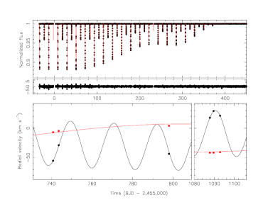
Figure 9.: Top: the normalized light curve of KIC 10319590 (points) with the best-fitting photodynamical model (red line). The units of the residuals are parts per thousand. Bottom: The radial velocities of the primary (black points) and the tertiary star (red points) and the best-fitting model curves.

KIC 7668648 shows a gradual increase in the eclipse depths and large ETVs (Figure 6). In addition, the third star transits both stars in the EB and is itself occulted by the other stars (Figure 7). Spectra were obtained using the echelle spectrograph on the Kitt Peak 4m telescope. The spectra are double-lined where both stars in the EB are detected. A good photodynamical model was developed, and we find masses of $M_{1}=0.849\,M_{\odot}$, $M_{2}=0.808\,M_{\odot}$, and $M_{3}=0.278\,M_{\odot}$, and radii of $R_{1}=1.010\,R_{\odot}$, $R_{2}=0.881\,R_{\odot}$, and $R_{3}=0.289\,R_{\odot}$. The mean periods are 27.094 days for the inner orbit and 206.4 days for the outer orbit. Figure 10 shows the best-fitting photodynamical model, and one can see that the transits and occultations are well-fit, as are all of the primary and secondary eclipses. There is an odd feature in this EB. The eclipse event near day $-23$ (labeled $P_{1}$) is deeper than the eclipse event near day $-9$ (labeled $S_{1}$), so the former was called a “primary” eclipse. The eclipse event labeled $P_{52}$ occurs 51 orbital periods later than $P_{1}$ and the eclipse event labeled $S_{51}$ likewise occurs 51 orbital periods later than $S_{1}$. However, $S_{52}$ is deeper than $P_{52}$, which means the roles of the primary and secondary eclipses have reversed! KIC 7668648 is a very important system as it has a relatively low-mass star with a good mass and radius determination and also from a dynamical point of view, as it is a relatively compact triple.

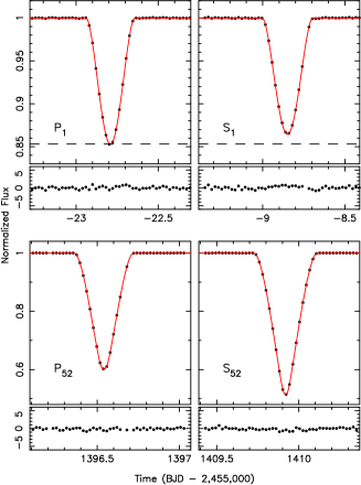
Figure 10.: Left: the normalized light curve of KIC 7668648 showing transits of the primary and secondary by the third body with the best-fitting photodynamical model (top) and occultations of the third star by the primary and secondary (bottom). Right: Close-up views of the first pair of primary and secondary eclipses (top) and the last pair of primary and secondary eclipses (bottom). Note that the roles of the primary and secondary eclipses have switched.

Acknowledgments

It is a pleasure to thank the many collaborators who have assisted with this work, including William Welsh, Donald Short, Gur Windmiller, and numerous students at San Diego State University, and members of the Kepler EB and TTV working groups including Andrej Prša, Laurance Doyle, Robert Slawson, Kyle Conroy, Steven Bloemen, Thomas Barclay, Joshua Pepper, David Latham, Tsevi Mazeh, Joshua Winn, Daniel Fabrycky, Joshua Carter, Jack Lissauer, Eric Ford, Eric Agol, Darin Ragozzine, Jason Steffen, Matt Holman, Billy Quarles, and Nader Haghighipour. We acknowledge support from the U.S. National Science Foundation (grants AST-1109928 and AST-0850564) and NASA (grant NNX12AD23G and the Kepler GO Program).

References

- Borkovits et al. (2003) Borkovits, T., Érdi, B., Forgács-Dajka, E., & Kovács, T. 2003, A&A, 398, 1091
- Borucki et al. (2010) Borucki, W. J., Koch, D., Basri, G., Batalha, N., Brown, T., et al. 2010, Science, 327, 977
- Carter et al. (2011) Carter, J. A., Fabrycky, D. C., Ragozzine, D., Holman, M., et al. 2011, Science, 331, 562
- Claret & Giménez (1992) Claret, A., & Giménez 1992, A&AS, 96, 255
- Conroy et al. (2014) Conroy, K., Prša, A., Stassun, K. G., Orosz, J. A., Fabrycky, D. C., & Welsh, W. F. 2014, AJ, 147, 45
- Doyle et al. (2011) Doyle, L. R., Carter, J. A., Fabrycky, D. C., Slawson, R. W., et al. 2011, Science, 333, 1602
- Fabrycky & Tremaine (2007) Fabrycky, D. C., & Tremaine, S. 2007, ApJ, 669, 1298
- Gies et al. (2012) Gies, D. R., Williams, S. J., Matson, R. A., Guo, Z, Thomas, S. M., et al. 2012, AJ, 143, 137
- Giménez & Garcia-Pelayo (1983) Giménez, A. & Garcia-Pelayo, J. M. 1983, Ap&SS, 92, 203
- Giménez (1985) Giménez, A. 1985, ApJ, 297, 405
- Graczyk et al. (2011) Graczyk, D., Soszyński, I., Poleski, R., Pietrzyński, G., Udalski, A., et al. 2011, AcA, 61, 103
- Irwin (1952) Irwin, J. B. 1952, AJ, 116, 211
- Kopal (1978) Kopal, Z. 1978, Dynamics of Close Binary Systems, (Dordrecht: D. Reidel Publishing Co.)
- Lacy (1992) Lacy, C. H. S. 1992, AJ, 104, 2213
- Mazeh & Shaham (1979) Mazeh, T., & Shaham, J. 1979, A&A, 77, 145
- Orosz & Hauschildt (2000) Orosz, J. A., & Hauschildt, P. H. 2000, A&A, 364, 265
- Orosz et al. (2012) Orosz, J. A., Welsh, W. F., Carter, J. A., Fabrycky, D. C., Cochran, W. D., et al. 2012, Science, 337, 1511
- Özdemir et al. (2003) Özdemir, S., Mayer, P., Drechsel, H., Demircan, O., & Ak, H. 2003, A&A, 403, 675
- Prša et al. (2011) Prša, A., Batalha, N., Slawson, R. W., Doyle, L. R., Welsh, W. F., et al. 2011, AJ, 141, 83
- Rappaport et al. (2013) Rappaport, S., Deck, S., Levine, A., Borkovits, T., Carter, J. et al. 2013, ApJ, 768, 33
- Sanchis-Ojeda et al. (2012) Sanchis-Ojeda, R., Fabrycky, D. C., Winn, J. N., Barclay, T., et al. 2012, Nature, 487, 449
- Slawson et al. (2011) Slawson, R. W., Prša, A., Welsh, W. F., Orosz, J. A., Rucker, M., et al. 2011, AJ, 142, 160
- Steffen et al. (2011) Steffen, J. H., Quinn, S. N., Borucki, W. J., et al. 2011, MNRAS, 417, L31
- Tokovinin et al. (2006) Tokovinin, A., Thomas, S., Sterzik, M., & Udry, S. 2006, A&A, 450, 657
- Torres & Stefanik (2000) Torres, G., & Stefanik, R. P. 2000, AJ, 119, 1914
- Torres (2001) Torres, G. 2001, AJ, 121, 2227