Fermion localization in higher curvature spacetime

Abstract

Fermion localization in a braneworld model in presence of dilaton coupled higher curvature Gauss-Bonnet bulk gravity is discussed. It is shown that the lowest mode of left handed fermions can be naturally localized on the visible brane due to the dilaton coupled higher curvature term without the necessity of any external localizing bulk field.

1 Introduction

Randall Sundrum warped geometry model Randall:1999ee ; Randall:1999vf is an eminently successul model in resolving the long standing gauge hierarchy/naturalness problem in an otherwise successful Standard model of elementary particles. This resulted in extensive search for a signature of Randall Sundrum (RS) model in Large Hadron Collider (LHC) Weiglein:2004hn ; Skittrall:2008pr ; DePree:2006ah ; Aad:2012cy ; Tang:2012pv ; Das:2013lqa . When applied as a physics beyond Standard Model (SM) such a scenario is often based on an underlying assumption that the SM fermions in general can propagate in the bulk while their chiral states are appropriately localized in different regions of bulk spacetime producing the desired 4-dimensional fermion masses on the visible brane. Though RS model itself can not provide any justification for this localization, there have been efforts to provide an explanation of this by introducing an ad-hoc scalar field in the anti- de Sitter bulk of RS model Bajc:1999mh ; Lehners:2007xa ; Chang:1999nh ; Koley:2004at ; ArkaniHamed:1999za ; Kaplan:2001ga ; Grossman:1999ra . Such a mechanism of localization however gives rise to the speculation about the possible back-reaction of the scalar to jeopardize the original RS solution for the warp factor. The origin of hierarchy of fermion masses in Standard model is a problem yet to be resolved. In this work we show that a string inspired modification to Einstein gravity via dilaton and higher curvature effects can explain the hierarchy among the fermion masses, where the effective masses of fermions are determined by their couplings with the dilaton field. Our work is staged on a five dimensional spacetime where our universe sits at one of the fixed points of the orbifolded extra spacetime dimension. This work thus is an attempt to look for an alternative pathway for this localization which resorts to the presence of higher curvature corrections to the classical Einsteinian gravity in the bulk as postulated in RS model. Such a correction, though heavily suppressed in low energy world, assumes significance in an Anti de Sitter (AdS) bulk with curvature $\sim$ Planck scale as assumed in RS model. At the leading order, such correction over Einstein Gravity which is free from the appearance of any ghost field due to the higher derivative terms, is the Gauss-Bonnet (GB) gravity where the various quadratic curvature terms appear in suitable combination to make the theory stable. Such a correction is also inspired by string theory which in addition also predicts the presence of the scalar dilaton in the action.

Following the path adopted in RS model, if the dilaton coupled GB gravity is compactified on $S^{1}/Z_{2}$ orbifold, it gives rise to two branches of warped solutions, one of which is stable and free of ghost. In this work we adopt this ghost free branch and study the effects of higher curvature couplings on the two chirality states of 5 dimensional SM fermions to study their localization on the standard model 3-brane.

As discussed earlier, if the standard model fermions also propagate in the bulk, just as graviton, then by appropriately choosing the interaction potential between the fermion and a localizing field one can try to obtain the appropriate overlap between the chiral states of the fermionic wave functions to localize the left chiral massless fermion states on the brane. However without resorting to any such external ad-hoc field can one produce this desired feature through the higher curvature GB terms in the bulk? This would then provide a natural explanation of observing only the left-handed neutrinos in our universe while the massive fermions appear with both the chiral states. We try to address this question in the present work in the framework of GB-dilaton induced warped geometry model Choudhury:2013yg .

In this work, we consider a bulk fermion and study the localization profile in the five dimensional warped geometry model in the backdrop of GB dilaton gravity. We will show that inclusion of higher curvature terms lead to the localization of left handed fermionic modes near the visible brane as their mass decreases while the right hand modes are localized within the bulk. In such localization scenario therefore one does not need to invoke an external bulk field as has been proposed earlier. Since the Standard model only includes the left handed modes of massless fermions, we can clearly see that this higher curvature setup will automatically allow the fermionic wave functions to localize themselves in the TeV brane. On the other hand, the delocalization of right handed modes inside the bulk can produce interesting phenomenological consequences like fermion mass generation as suggested by Ref. Grossman:1999ra .

2 Fermion localization in Gauss-Bonnet dilaton gravity

Here we generalize the analysis in warped geometry in presence of Gauss-Bonnet coupling and gravidilaton coupling in a 5D bulk. The background warped geometry model is proposed by making use of the following sets of assumptions as a building block:

• The leading order Einstein’s gravity sector is modified by the GB Choudhury:2012yh ; Choudhury:2013qza ; Choudhury:2013eoa ; Choudhury:2013dia ; Choudhury:2013yg ; Kim:1999dq ; Lee:2000vf ; Kim:2000pz ; Kim:2000ym and dilaton coupling Choudhury:2013eoa ; Choudhury:2013dia ; Choudhury:2013yg ; Choudhury:2013aqa which originates from heterotic string theory.

• The background warped metric has a RS like structure Randall:1999ee ; Randall:1999vf on a slice of ${\bf AdS_{5}}$ geometry. For example, from 10-dimensional string model compactified on ${\bf AdS_{5}\times S^{5}}$, one typically obtains moduli from ${\bf S^{5}}$ as scalar degrees of freedom. Such moduli can be stabilized by fluxes. In our model, which is similar to a 5-dimensional Randall-Sundrum (RS) model, it is assumed that these degrees of freedom are frozen to their Vacuum expectation value (VEV) and are non-dynamical at the energy scale under consideration Reece:2010xj . We therefore focus into the slice of ${\bf AdS_{5}}$ as is done for the 5-dimensional RS model.

• The well known ${\bf S^{1}/Z_{2}}$ orbifold compactification is considered.

• The dilaton degrees of freedom is assumed to be confined within the bulk.

• We allow the interaction between dilaton and the 5D bulk cosmological constant via dilaton coupling.

• The Higgs field is localized at the visible (TeV) brane and the hierarchy problem is resolved via Planck to TeV scale warping.

• The modulus can be stabilized by introducing scalar in the ${\bf AdS_{5}}$ bulk without any fine tuning following Goldberger-Wise (GW) mechanism Goldberger:1999uk ; Goldberger:1999un ; Goldberger:1999wh ; Choudhury:2014hna .

• Additionally while determining the values of the model parameters we require that the bulk curvature to be less than the five dimensional Planck scale $M_{5}$ so that the classical solution of the 5-dimensional gravitational equations can be trusted Davoudiasl:1999jd ; Das:2013lqa .

2.1 The background setup

Before going to discuss the various features of fermion localization, we start with the 5D action for the two brane warped geometry model including higher curvature gravity as Choudhury:2013yg :

$$\begin{array}[]{llll}\displaystyle S=\int d^{5}x\left[\sqrt{-g_{(5)}}\left\{\frac{M^{3}_{(5)}}{2}R_{(5)}+\frac{\alpha_{(5)}M_{(5)}}{2}\left[R^{ABCD(5)}R^{(5)}_{ABCD}-4R^{AB(5)}R^{(5)}_{AB}+R^{2}_{(5)}\right]\right.\right.\\ \left.\left.\displaystyle~{}~{}~{}~{}~{}~{}~{}~{}~{}~{}~{}~{}~{}~{}~{}~{}~{}~{}~{}~{}~{}~{}~{}~{}~{}~{}~{}~{}~{}~{}-M^{3}_{(5)}\frac{g^{AB}}{2}\partial_{A}\chi(y)\partial_{B}\chi(y)-2\Lambda_{5}e^{\chi(y)}\right\}-\displaystyle\sum^{2}_{i=1}\sqrt{-g^{(i)}_{(5)}}T_{i}e^{\chi(y)}\delta(y-y_{i})\right]\end{array}$$ (1)

where $A,B,C,D=0,1,2,3,4$. Here $i$ signifies the brane index, $i=1(\text{hidden})$, $2(\text{visible})$ and $T_{i}$ is the brane tension. Additionally $\alpha_{5}$ and $\chi(y)$ represent the Gauss-Bonnet coupling and dilaton. The background metric describing slice of the ${\bf AdS_{5}}$ is given by,

$$\begin{array}[]{llllll}\displaystyle ds^{2}_{5}=g_{AB}dx^{A}dx^{B}=e^{-2k_{\bf M}(y)r_{c}|y|}\eta_{\alpha\beta}dx^{\alpha}dx^{\beta}+r^{2}_{c}dy^{2}\end{array}$$ (2)

where $r_{c}$ represents the compactification radius of extra dimension which has a unit of $M^{-2}_{pl}$. Here the orbifold points are $y_{i}=[0,\pi]$ and periodic boundary condition is imposed in the closed interval $-\pi\leq y\leq\pi$. After orbifolding, the size of the extra dimensional interval is $\pi r_{c}$. Here it is important to note that, the bulk extra dimension $y$ is dimensionless and plays a role of an angular coordinate in this conetext. Moreover in the above metric ansatz $e^{-2A(y)}$ represents the warp factor while $\eta_{\alpha\beta}=(-1,+1,+1,+1)$ is flat Minkowski metric. A more general brane metric for a purely Einsteinian bulk has been discussed in Koley:2010za .

2.2 Warp factor from Gauss-Bonnet dilaton gravity

After varying the model action stated in Eq (1) we get:

$$\begin{array}[]{lllll}\delta S=\displaystyle\int d^{5}x\left[\sqrt{-g_{(5)}}\left\{M^{3}_{(5)}G^{(5)}_{AB}+\alpha_{(5)}M_{(5)}H^{(5)}_{AB}+T_{AB}\right\}+\sum^{2}_{i=1}T_{i}\sqrt{-g^{(i)}_{(5)}}g^{(i)}_{\alpha\beta}\delta^{\alpha}_{A}\delta^{\beta}_{B}e^{\chi(y)}\delta(y-y_{i})\right]\delta g^{AB}\\ \displaystyle~{}~{}~{}~{}~{}~{}~{}~{}~{}~{}~{}~{}~{}~{}~{}+\int d^{5}x\left[\sqrt{-g_{(5)}}\left\{-M^{3}_{(5)}\Box_{(5)}\chi-2\Lambda_{(5)}e^{\chi(y)}\right\}+\sum^{2}_{i=1}T_{i}\sqrt{-g^{(i)}_{(5)}}e^{\chi(y)}\delta(y-y_{i})\right]\delta\chi\end{array}$$ (3)

where the five dimensional Einstein’s tensor, the Gauss-Bonnet tensor are given by:

$$\begin{array}[]{llll}G^{(5)}_{AB}=\left[R^{(5)}_{AB}-\frac{1}{2}g^{(5)}_{AB}R_{(5)}\right],\end{array}$$ (4)

and

$$\begin{array}[]{llll}H^{(5)}_{AB}=2R^{(5)}_{ACDE}R_{B}^{CDE(5)}-4R_{ACBD}^{(5)}R^{CD(5)}-4R_{AC}^{(5)}R_{B}^{C(5)}+2R^{(5)}R_{AB}^{(5)}\\ ~{}~{}~{}~{}~{}~{}~{}~{}~{}~{}~{}~{}~{}~{}~{}~{}~{}~{}~{}~{}~{}~{}~{}~{}~{}~{}~{}~{}~{}~{}~{}~{}~{}~{}~{}~{}~{}~{}~{}~{}~{}~{}~{}-\frac{1}{2}g^{(5)}_{AB}\left(R^{ABCD(5)}R^{(5)}_{ABCD}-4R^{AB(5)}R^{(5)}_{AB}+R^{2}_{(5)}\right).\end{array}$$ (5)

Also the 5D D’Alembertian operator is defined as, $\Box_{(5)}\chi(y)=\frac{1}{\sqrt{-g_{(5)}}}\partial_{A}\left(\sqrt{-g_{(5)}}\partial^{A}\chi(y)\right)$. In this context the 5D dilaton stress tensor is defined as, $T_{AB}=-\frac{2}{\sqrt{-g_{(5)}}}\frac{\delta}{\delta g^{AB}}\left(\sqrt{-g_{(5)}}{\cal L}_{\chi}\right)$, where ${\cal L}_{\chi}$ is dilaton Lagrangian as given by, ${\cal L}_{\chi}=\left[-M^{3}_{(5)}\frac{g^{AB}}{2}\partial_{A}\chi\partial_{B}\chi-V(\chi)\right]$. Here it is important to note that the 5D bulk dilaton potential is identified to be the following expression: $V(\chi)=2\Lambda_{5}e^{\chi(y)}$, where 5D cosmological constant $\Lambda_{(5)}$ fix the scale of the dilaton potential.

By doing explicit computation one can show that the 5D dilaton stress tensor can be expressed as:

$$T_{AB}=\left[\partial_{A}\chi(y)\partial_{B}\chi(y)+g_{AB}\left(\frac{g_{CD}}{2}\partial_{C}\chi(y)\partial_{D}\chi(y)+V(\chi)\right)\right].$$ (6)

After varying the model action stated in equation(1) with respect to the 5D metric $g_{AB}$ we get, $\frac{\delta S}{\delta g^{AB}}=0$ using which the 5D bulk equation of motion turns out to be,

$$\begin{array}[]{lllll}\displaystyle\sqrt{-g_{(5)}}\left[G^{(5)}_{AB}+\frac{\alpha_{(5)}}{M^{2}_{(5)}}H^{(5)}_{AB}\right]=-\frac{1}{M^{3}_{(5)}}\left[\sqrt{-g_{(5)}}~{}T_{AB}+\sum^{2}_{i=1}T_{i}\sqrt{-g^{(i)}_{(5)}}g^{(i)}_{\alpha\beta}\delta^{\alpha}_{A}\delta^{\beta}_{B}e^{\chi(y)}\delta(y-y_{i})\right].\end{array}$$ (7)

Now very far from the orbifold points the 5D field equation in the warped background can be simplified in the following form:

$$\begin{array}[]{lllll}\displaystyle\sqrt{-g_{(5)}}\left[G^{(5)}_{AB}+\frac{\alpha_{(5)}}{M^{2}_{(5)}}H^{(5)}_{AB}\right]=-\frac{1}{M^{3}_{(5)}}\sqrt{-g_{(5)}}~{}T_{AB}.\end{array}$$ (8)

Similarly varying equation(1) with respect to the dilaton field we get, $\frac{\delta S}{\delta\chi}=0$. using which the Klein Gordon (KG) equation for the dilaton in the warped background turns out to be:

$$\begin{array}[]{llll}\displaystyle\frac{1}{M^{3}_{(5)}}\sum^{2}_{i=1}T_{i}\sqrt{-g^{(i)}_{(5)}}e^{\chi(y)}\delta(y-y_{i})=\sqrt{-g_{(5)}}\left\{\displaystyle 2\frac{\Lambda_{(5)}}{M^{3}_{(5)}}e^{\chi(y)}+\Box_{(5)}\chi\right\}.\end{array}$$ (9)

Now very far from the orbifold points the KG equation for the dilaton in the warped background can be simplified in the following form:

$$\begin{array}[]{llll}\displaystyle\Box_{(5)}\chi=J(\chi).\end{array}$$ (10)

Here $J(\chi)$ is identified to be the source function for the bulk localized dilaton field, which is given by the following expression:

$$J(\chi)=\frac{V(\chi)}{M^{3}_{(5)}}=2\frac{\Lambda_{(5)}}{M^{3}_{(5)}}e^{\chi(y)}.$$ (11)

Before solving the Eq (7) and Eq (10), here it is important to note that the following crucial facts which are surely be helpful for us to understand the nature of the field equations:

• First of all the derived two field equations are second order coupled differential equations. Here such complicated structures are appearing due to minimal interaction between gravity and dilaton in the bulk.

• On the other hand, the KG equation for the dilaton in the warped background is itself complicated as it contains an exponential source term, which is appearing as dilaton effective potential in the bulk.

• Both of the equations can be simplified as Eq (8) and Eq (10) if we go very far drom the orbifold fixed points.

In order to solve these coupled equations, we use some approximations as follows : First of all, it is important to note that we may neglect the derivative terms in the dilaton action with respect to it’s potential which is of the order of Planck scale. Due to this fact the stress energy tensor of the dilaton approximately, is given by the expression:

$$T_{AB}\approx g_{AB}V(\chi)=2g_{AB}\Lambda_{(5)}e^{\chi(y)}.$$ (12)

Consequently, the 5D field equation can be be recast into the following simplified form:

$$\begin{array}[]{lllll}\displaystyle\sqrt{-g_{(5)}}\left[G^{(5)}_{AB}+\frac{\alpha_{(5)}}{M^{2}_{(5)}}H^{(5)}_{AB}\right]\approx-\frac{e^{\chi(y)}}{M^{3}_{(5)}}\left[\Lambda_{(5)}\sqrt{-g_{(5)}}g^{(5)}_{AB}+\sum^{2}_{i=1}T_{i}\sqrt{-g^{(i)}_{(5)}}g^{(i)}_{\alpha\beta}\delta^{\alpha}_{A}\delta^{\beta}_{B}\delta(y-y_{i})\right],\end{array}$$ (13)

which can be further simplified in the region far away from the orbifold fixed points as:

$$\begin{array}[]{lllll}\displaystyle\sqrt{-g_{(5)}}\left[G^{(5)}_{AB}+\frac{\alpha_{(5)}}{M^{2}_{(5)}}H^{(5)}_{AB}\right]\approx-\frac{e^{\chi(y)}}{M^{3}_{(5)}}\sqrt{-g_{(5)}}~{}\Lambda_{(5)}g^{(5)}_{AB}=-\frac{1}{M^{3}_{(5)}}\sqrt{-g_{(5)}}~{}V(\chi)g^{(5)}_{AB}.\end{array}$$ (14)

Moreover, considering the equation of motion for the dilaton , we further note that the source term in the right hand side is extremely suppressed due to the warping and therefore may be neglected. As a result the space variation of $\chi(y)$ can be derived from the equation:

$$\begin{array}[]{llll}\displaystyle\partial^{2}_{y}\chi(y)\approx 0.\end{array}$$ (15)

Now using the ${\bf Z_{2}}$ orbifolding, we obtain at the leading order of $\alpha_{(5)}$ Choudhury:2013yg :

$$\begin{array}[]{llll}\displaystyle\boxed{\chi(y)=\left(c_{1}|y|+c_{2}\right)}\end{array}$$ (16)

where $c_{1}$ and $c_{2}$ are arbitrary integration constants in which $c_{1}$ characterizes the strength of the dilaton self interaction within the bulk. For our computation we fix $c_{2}=0$. As the nature of warping influences the localization profile of the bulk fermion, therefore it is expected that the dilaton charge $c_{1}$ for a given fermionic field will determine the localization property and hence the effective fermion mass term on the brane.

The corresponding warp factor turns out to be Choudhury:2013yg :

$$\begin{array}[]{llll}\displaystyle A(y):=A_{\pm}(y)=k_{\pm}(y)r_{c}|y|\end{array}$$ (17)

where

$$\begin{array}[]{llll}\displaystyle\boxed{k_{\pm}(y)=\sqrt{\frac{3M^{2}_{(5)}}{16\alpha_{(5)}}\left[1\pm\sqrt{\left(1+\frac{4\alpha_{(5)}\Lambda_{5}e^{\chi(y)}}{9M^{5}_{(5)}}\right)}\right]}}~{}.\end{array}$$ (18)

Also the localized brane tensions are given by:

$$\boxed{T_{2}=-T_{1}=24k_{\pm}(y)M^{3}_{(5)}~{}e^{-\chi(y)}\left[1-\frac{\alpha_{(5)}}{3M^{2}_{(5)}}k^{2}_{\pm}(y)r^{2}_{c}\right]}~{}.$$ (19)

In the small $\alpha_{(5)}$, $c_{1}$ and $c_{2}$ limit we retrieve the results as in the case of RS model with:

$$k_{-}(y)\rightarrow k_{RS}=\sqrt{-\frac{\Lambda_{5}}{24M^{3}_{(5)}}}.$$ (20)

and the corresponding brane tension is given by:

$$T^{RS}_{2}=-T^{RS}_{1}=24k_{RS}M^{3}_{(5)}.$$ (21)

Here we have discarded the +ve branch of solution of $k_{+}$ which diverges in the small $\alpha_{(5)}$ limit, bringing in ghost fields Rizzo:2004rq ; Dotti:2007az ; Torii:2005xu ; Konoplya:2010vz ; Kim:2000ym ; Nojiri:2010wj . Now expanding Eq (18) in the perturbation series order by order around $\alpha_{5}\rightarrow 0$, $c_{1}\rightarrow 0$ and $c_{2}\rightarrow 0$ we can write:

$$\displaystyle\boxed{k_{\bf M}(y):=k_{-}(y)=k_{RS}~{}e^{\frac{\chi(y)}{2}}\left[1+{\bf L}+{\cal O}({\bf L}^{2})+\cdots\right]}~{}.$$ (22)

where ${\bf L}$ is defined as:

$${\bf L}:=\frac{4\alpha_{(5)}k^{2}_{RS}}{M^{2}_{(5)}}.$$ (23)

However, the results of this paper will be unchnaged if we take the non zero value of the constant $c_{2}$. In the weak coupling regime of gravity and dilaton one can also consider non zero but small values of $c_{2}$ which is finally appearing as an overall factor $e^{c_{2}/2}$ in the expression for the warp factor in Eq (22). More precisely the contribution in the warp factor can be written as:

$$e^{c_{2}/2}\approx 1+\underbrace{\left(\frac{c_{2}}{2}+\cdots\right)}_{\bf<<1~{}in~{}weak~{}coupling}\approx\left(1+\frac{c_{2}}{2}\right),$$ (24)

where we have neglected all the higher powers of $c_{2}$ as in the weak coupling regime of the gravity and dilaton always $c_{2}<<1$ approximation holds good. On the other hand it is important to note that, in this context strictly one cannot consider very large values of $c_{2}$ as in that case the perturbative solution in the weak coupling approximation itself is not valid for dilaton and consequently in the solution for the warp factor. Additionally in the weak coupling regime of gravity and dilaton the dilatonic charge $c_{1}$ is small compared to unity at the orbifold point $y=\pi$ where the visible brane is placed. Here to visualize the effect of dilaton in the phenomena of localization of fermions we further use an approximation that the contribution from the dilatonic charge $c_{1}$ is larger than the contribution from $c_{2}$ at the orbifold point $y=\pi$. For the similar reason here also large values of $c_{1}$ is not strictly allowed. Using these set of approximations one can finally write down the warp function as:

$$\displaystyle k_{\bf M}(y)\approx k_{RS}~{}e^{\frac{c_{1}y}{2}}\left(1+\frac{c_{2}}{2}\right)\left[1+{\bf L}+{\cal O}({\bf L}^{2})+\cdots\right].$$ (25)

Further Eq (25) can be used to solve the naturalness or gauge hierarchy problem and for this purpose one need to consider the following modified constraint at the orbifold point $y=\pi$ as given by:

$$k_{\bf M}(\pi)r_{c}\approx k_{RS}r_{c}e^{c_{1}\pi/2}\left(1+\frac{c_{2}}{2}\right)\left[1+{\bf L}+{\cal O}({\bf L}^{2})+\cdots\right]\approx 12.$$ (26)

As in the weak coupling regime the constant $c_{2}$ is just playing the role of a correction term or an overall normalization factor, one can neglect the contribution from the coupling $c_{2}$ completely without taking care of any small contributions from the small corrections. This is exactly equivalent to the similar effect if we set $c_{2}=0$ from the strating point of our computation. In this case Eq (25) can be written as:

$$\displaystyle\boxed{k_{\bf M}(y)\approx k_{RS}~{}e^{\frac{c_{1}y}{2}}\left[1+{\bf L}+{\cal O}({\bf L}^{2})+\cdots\right]}~{},$$ (27)

and consequently the modified constraint condition to solve the naturalness or gauge hierarchy problem can be recast at the orbifold point $y=\pi$ as:

$$\boxed{k_{\bf M}(\pi)r_{c}\approx k_{RS}r_{c}e^{c_{1}\pi/2}\left[1+{\bf L}+{\cal O}({\bf L}^{2})+\cdots\right]\approx 12}~{}.$$ (28)

Now if we set the limit $\alpha_{5}\rightarrow 0$ and $c_{1}\rightarrow 0$ then one can get back the RS result, which is $k_{RS}r_{c}\approx 12$. Here it is important to note that, both the solution of the warp factor and the dilaton is consistent with Eq (14) and Eq (15) in the weak coupling regime of gravity (graviton) and dilaton in the bulk.

2.3 Localization scenario for fermions

We will now start our discussion regarding the localization scenario of fermionic modes. The five dimensional action for the massive fermionic field can be written as:

$$\begin{array}[]{llll}\displaystyle S_{f}=\int d^{5}x\left[Det({\cal V})\right]~{}\left\{i\bar{\Psi}(x,y)\gamma^{\alpha}{\cal V}_{\alpha}^{M}\overleftrightarrow{{\large\bf D}_{\mu}}\Psi(x,y)\delta^{\mu}_{M}-sgn(y)m_{f}\bar{\Psi}(x,y)\Psi(x,y)+~{}h.c.\right\}\\ \displaystyle~{}~{}~{}=\int d^{5}x~{}e^{-4k_{\bf M}(y)r_{c}|y|}\left\{\bar{\Psi}(x,y)\left[ie^{k_{\bf M}(y)r_{c}|y|}\gamma^{\mu}\partial_{\mu}\right.\right.\\ \left.\left.\displaystyle~{}~{}~{}~{}~{}~{}~{}~{}~{}~{}~{}~{}~{}~{}~{}~{}~{}~{}~{}~{}~{}~{}~{}~{}~{}~{}~{}~{}~{}~{}~{}~{}~{}+\gamma^{5}(\partial_{y}-2r_{c}\partial_{y}\{k_{\bf M}(y)|y|\})-sgn(y)m_{B}\right]{\Psi}(x,y)+h.c.\right\}\end{array}$$ (29)

where the differential operator $\overleftrightarrow{{\large\bf D}_{\mu}}$ ise defined as, $\overleftrightarrow{{\large\bf D}_{\mu}}:=\left(\overleftrightarrow{\partial_{\mu}}+\Omega_{\mu}\right)$, which represents the covariant derivative in presence of fermionic spin connection:

$$\Omega_{\mu}=\frac{1}{8}\omega_{\mu}^{\hat{A}\hat{B}}\left[\Gamma_{\hat{A}},\Gamma_{\hat{B}}\right].$$ (30)

Here $\omega_{\mu}^{\hat{A}\hat{B}}$ represents the gauge field respecting ${\cal SO}(3,1)$ transformation on the vierbein coordinate. Here we assume that the bulk fermion mass $m_{B}$ originates through an underlying spontaneous symmetry breaking in bulk via 5-dimensional Higgs mechanism Dey:2009gf ; Huber:2000fh ; Chang:1999nh ; Chang:2000zh ; Davoudiasl:2005uu . The 5D Gamma matrices:

$$\Gamma^{\hat{A}}=\left(\gamma^{\mu},\gamma_{5}:=\frac{i}{4!}{\bf\epsilon}_{\mu\nu\alpha\beta}\gamma^{\mu}\gamma^{\nu}\gamma^{\alpha}\gamma^{\beta}=i\gamma_{4}\right)$$ (31)

satisfy the Clifford algebra anti-commutation relation $\{\Gamma^{\hat{A}},\Gamma^{\hat{B}}\}=2\eta^{\hat{A}\hat{B}}$ with $\eta^{\hat{A}\hat{B}}=$
$diag\left(-1,+1,+1,+1,+1\right)$. In this context

$$g_{MN}:=\left({\cal V}_{M}^{\hat{A}}\otimes{\cal V}_{N}^{\hat{B}}\right)\eta_{\hat{A}\hat{B}},$$ (32)

where ${\cal V}_{M}^{\hat{A}}$ are characterized by the usual conditions:

$$\displaystyle{\cal V}_{4}^{4} = 1,$$ (33)

$${\cal V}_{\mu}^{\hat{A}} = e^{k_{\bf M}(y)r_{c}|y|}\delta_{\mu}^{\hat{A}},$$ (34)

$$Det({\cal V}) = e^{-4k_{\bf M}(y)r_{c}|y|}.$$ (35)

and $\hat{A},\hat{B}$ being tangent space indices. For our set up ${\cal SO}(3,1)$ spin connection can be written as:

$$\Omega_{4} = 0,$$ (36)

$$\Omega_{\mu} = -\frac{1}{2}e^{-k_{\bf M}(y)r_{c}|y|}k_{\bf M}(y)r_{c}\gamma_{5}\gamma_{\mu}.$$ (37)

Here focusing our attention only to the lowest fermionic mode in the brane. To serve this purpose we decompose the five-dimensional spinor as

$$\Psi(x,y)=\psi(x)\xi(y).$$ (38)

In the massless case the definite chiral states $\psi_{L}(x)$ and $\psi_{R}(x)$ correspond to left and right chiral states in four dimension. The $\psi_{L}$ and $\psi_{R}$ are constructed by,

$$\psi_{L,R}=\frac{1}{2}(1\mp\gamma^{5})\psi.$$ (39)

Here $\xi$ denotes the extra dimensional component of the fermion wave function. We then can decompose five-dimensional spinor in the following way:

$$\Psi(x,y)=\psi_{L}(x)\xi_{L}(y)+\psi_{R}(x)\xi_{R}(y)$$ (40)

Substituting the above decomposition in Eq (29) we obtain the following equations for the fermions,

$$\begin{array}[]{lll}\displaystyle e^{-k_{\bf M}(y)r_{c}|y|}\left[\pm(\partial_{y}-2r_{c}\partial_{y}\{k_{\bf M}(y)|y|\})+sgn(y)m_{B}\right]\xi_{R,L}(y)=-m~{}\xi_{L,R}(y)\end{array}$$ (41)

where $m_{B}$ and $m$ represent the 5D bulk mass and lowest effective mass of 4D fermion respectively. The 4D fermions obey the canonical equation of motion, $i\gamma^{\mu}\partial_{\mu}\psi_{L,R}=m\psi_{L,R}$. Also it is important note that the left and right handed part of the extra dimensional wave function satisfies the usual ortho-normality condition. Finally, the solution of Eq (41) turns out to be:

$$\begin{array}[]{lll}\boxed{\xi_{L,R}(y)={\cal N}\text{exp}\left[2~{}e^{\frac{\chi(y)}{2}}k_{\bf M}(y)|y|r_{c}\pm m\int dy~{}e^{k_{\bf M}(y)r_{c}|y|}\pm sgn(y)m_{B}|y|\right]}\end{array}$$ (42)

where ${\cal N}$ represents the normalization constant .

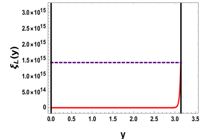
(a) Left fermionic mode with $m\sim{\cal O}({\rm TeV})$.

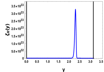
(b) Right fermionic mode with $m\sim-{\cal O}({\rm TeV})$.

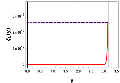
(c) Leftt fermionic mode with $m\sim{\cal O}({\rm GeV})$.

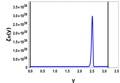
(d) Right fermionic mode with $m\sim-{\cal O}({\rm GeV})$.

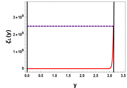
(e) Left fermionic mode with $m\sim{\cal O}({\rm MeV})$.

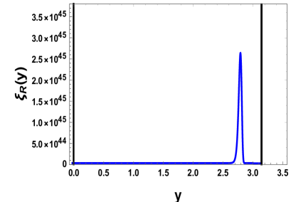
(f) Right fermionic mode with $m\sim-{\cal O}({\rm MeV})$.

Figure 1: Localization of the left and right handed fermionic profile $\xi_{L,R}(y)$. For all situations we have taken $\alpha_{(5)}=10^{-3}$, $c_{1}=0.17$, $m_{B}=(+1(left),-1(right))$ which fixes, $k_{\bf M}r_{c}=12$, is necessarily required to solve the hierarchy problem. Here all the masses are given in the Planckian unit. The black colored vertical lines represents the hidden and visible branes which are placed at the orbifold points $y=0$ and $y=\pi$ respectively. Also the purple colored dashed line represent that left handed mode always touches the visible brane at $y=\pi$ with a finite hight of the wave function.

Fig. (1(a)-1(f)) describe the localization profiles of the fermion wave function inside the bulk. They clearly depict that for both massive as well as massless fermions, the left handed mode is localized on the brane while the right handed fermions are localized inside the bulk. Additionally, from the prescribed analysis we can observe that the gradual increment in the dilaton coupling $c_{1}$ for a fixed value of Gauss Bonnet parameter ${\bf L}$ within the window :

$$10^{-3}<{\bf L}<10^{-7},$$ (43)

will shift the peak position of the right handed fermionic wave function towards left side of the visible brane towards the bulk. In such a situation the hight of the right fermionic mode increases, amount of localization increases and the localization position of the left fermionic mode slightly shift from the visible brane towards the bulk. Here it is clear from the Fig. (1(a)-1(f)), the mass of the different generation fermions increases from MeV to TeV, the wave function gets more and more sharply peaked towards the visible brane, implying more localization. We also observe that the the effective 4D mass $m$ term decreases as the peak position of the left handed fermionic mode shifts towards visible brane. Additionally it is important to note that left handed mode always touches the visible brane at $y=\pi$ with a finite hight of the wave function for the different values of the effective 4D mass $m$ lying within MeV to TeV window.

Serial	Constraint on	Different sources for	Final
number	GB coupling	the constraint on GB coupling	remarks
	$({\bf{\color[rgb]{1,0,0}\bf L}})$
I.	$0-10^{-7}$	Perihelion precession of planetary orbits	Astrophysical
		and the bending angle of null geodesics.	constraint.
II.	$10^{-7}-0.2$	The disovered Higgs mass	LHC
		and Higss diphoton and dilepton	constraint.
		decays using ATLAS and CMS data.
III.	$(4.8-5.1)\times 10^{-7}$	Lower bound on the lightest KK graviton mass	Search for
		from ATLAS dilepton search.	extra dimensions at LHC.
IV.	$<0.25$	Positivity of viscosity entropy ratio	AdS/CFT
			correspondense.
V.	$10^{-3}-10^{-7}$	Localization of lowest mode of left handed	Constraint from extra
		fermions without using any bulk field.	dimensions and
			consistent with
			I,II,III,IV.

Table 1: Various constraints on GB coupling from different sources.

Additionally it is important to note that, from various experiments and observations following constraints are available for the Gauss Bonnet parameter ${\bf L}\sim\alpha_{(5)}$ (where $k_{RS}\sim M_{(5)}$), which are perfectly consistent with the present window of the the Gauss Bonnet parameter considered in this paper:

• Astrophysical constraints from the perihelion precession of planetary orbits and the bending angle of null geodesics suggests that the bound on the Gauss Bonnet parameter ${\bf L}\sim\alpha_{(5)}$ lie within the following window Chakraborty:2012sd :

  $$0<{\bf L}<10^{-7}.$$ (44)

• Collider constraints from the Higgs mass of the resonance discovered near 125 GeV and the constraints from the $\mu$ parameter for Higss diphoton and dilepton decays using ATLAS Aad:2012tfa and CMS Chatrchyan:2013lba data within the $5\sigma$ statistical C.L. suggests that the bound on the Gauss Bonnet parameter ${\bf L}\sim\alpha_{(5)}$ lie within the following window Choudhury:2013eoa :

  $$10^{-7}<{\bf L}<0.2.$$ (45)

• Another phenomenological constraint from the the lower bound on the lightest Kaluza-Klein (KK) graviton mass as obtained from the ATLAS Aad:2012tfa dilepton search in 7 TeV proton-proton collision suggests that the bound on the Gauss Bonnet parameter ${\bf L}\sim\alpha_{(5)}$ lie within the following window Choudhury:2013eoa :

  $$4.8\times 10^{-7}<{\bf L}<5.1\times 10^{-7}.$$ (46)

• In the context of AdS/CFT the viscosity entropy ratio can be computed in presence of Gauss Bonnet parameter ${\bf L}\sim\alpha_{(5)}$ using the well known Kubo formula as Choudhury:2013dia ; Brigante:2007nu :

  $$\frac{\eta}{S}=\frac{1}{4\pi}(1-4{\bf L})+{\cal O}({\bf L}^{2}).$$ (47)

  To satisfy the constraint on the positivity of the viscosity entropy ratio the upper bound on the Gauss Bonnet parameter ${\bf L}\sim\alpha_{(5)}$ is given by Choudhury:2013eoa ; Brigante:2007nu :

  $${\bf L}<0.25.$$ (48)

In table (1) for the comparison of different sources of contraints on GB coupling we have mentioned all of these results, which shows that the result obtained in this paper is perfectly consistent with the astrophysical and particle collider data.

The overlap wave function of the left and right handed mode on the visible brane determines the effective mass of the fermion on the 3 brane. The effective 4D mass can be computed from the overlap integral as:

$$\displaystyle{\bf I}_{overlap} = m_{B}\int d^{5}x\left[Det({\cal V})\right]~{}sgn(y)\bar{\Psi}(x,y){\Psi}(x,y)$$ (49)

$$= \int d^{4}x~{}m_{L,R}\left[\bar{\Psi}_{L}(x){\Psi}_{R}(x)+\bar{\Psi}_{R}(x){\Psi}_{L}(x)\right],$$

where the 4D effective mass $m_{L,R}$ is given by:

$$\begin{array}[]{lllll}\displaystyle m_{L,R}=m_{B}\int^{\pi}_{0}dy~{}e^{-4k_{\bf M}(y)r_{c}|y|}sgn(y)\xi^{\dagger}_{L}(y)\xi_{R}(y).\end{array}$$ (50)

Above equation clearly indicates that if the bulk mass $m_{B}=0$ , then the mass of the lowest mode of fermions will also be zero. Further substituting Eq (42) in Eq (50) the effective mass $m=m_{L,R}$ can be recast as:

$$\begin{array}[]{llll}\displaystyle\boxed{m=2m_{B}\frac{\sqrt{5\left[1+{\bf L}+{\cal O}({\bf L}^{2})\right]}\exp\left[\left\{48\pi~{}e^{\frac{c_{1}\pi}{2}}\left(e^{\frac{c_{1}\pi}{2}}-1\right)+\frac{6}{5c_{1}}\right\}\left[1+{\bf L}+{\cal O}({\bf L}^{2})\right]\right]}{\sqrt{\frac{\pi}{6c_{1}}}\left(\text{Erfi}\left[\frac{\sqrt{6}\sqrt{\left[1+{\bf L}+{\cal O}({\bf L}^{2})\right]}}{\sqrt{5c_{1}}}\right]-\text{Erfi}\left[\frac{\sqrt{6}\sqrt{\left[1+{\bf L}+{\cal O}({\bf L}^{2})\right]}\left(1+5c_{1}\pi\right)}{\sqrt{5c_{1}}}\right]\right)}}\end{array}$$ (51)

where we fix $k_{RS}r_{c}=12$, which is necessary condition to resolve the gauge hierarchy or naturalness problem. In Eq. (51), we have introduced imaginary error function, which is defined as:

$$\text{Erfi}(x) = -i~{}\text{Erfi}(ix)=\frac{2}{\sqrt{\pi}}e^{x^{2}}~{}{\cal D}(x)$$ (52)

where ${\cal D}(x)$ is the Dwason function, is given by:

$${\cal D}(x) = e^{-x^{2}}\int^{x}_{t=0}e^{t^{2}}~{}dt.$$ (53)

4D mass	5D bulk	GB	Dilaton
	mass	coupling	coupling
${\color[rgb]{1,0,0}\bf m}$	${\color[rgb]{0,0,1}m_{\bf B}}$	${\color[rgb]{.75,0,.25}\bf L}$	${\bf c_{1}}$
(in  ${\rm GeV}$)	(in  $M_{Pl}$)
$10^{3}$	1	$10^{-3}-10^{-7}$	0.007
$1$	1	$10^{-3}-10^{-7}$	0.033
$10^{-3}$	1	$10^{-3}-10^{-7}$	0.057
$10^{-6}$	1	$10^{-3}-10^{-7}$	0.078
$10^{-9}$	1	$10^{-3}-10^{-7}$	0.098

Table 2: Parameter space required to generate overlap of left and right handed fermion wave functions at the visible brane via 4D effective mass.

In table (2) we have shown the total parameter space for the GB coupling ${\bf L}$, dilaton coupling $c_{1}$ and the 5D bulk mass $m_{\bf B}$ required to generate the overlap of left and right handed fermion wave functions at the visible brane via arying the 4D effective mass within the window $10^{-9}~{}{\rm GeV}<m<10^{3}~{}{\rm GeV}$.

3 Conclusion

The localization of left handed standard model fermions requires an external 5D bulk field. In this work, we have shown that it is possible to localize the SM fermions in the bulk using the higher curvature dilaton coupled gravity set-up without invoking any external scalar field in the bulk. This, then naturally explains the origin of localization of left handed fermions in the visible brane whereas the right handed fermionic modes get delocalized and obtain their peak inside the bulk. We have also obtained the effective 4D mass term in the brane which depends on the GB coupling parameters and dilaton coupling. Thus a string inspired background with higher curvature Gauss-Bonnet term and dilaton field in the bulk offers a natural explanation for the fermion localization on our brane.

References

- (1) L. Randall and R. Sundrum, “A Large mass hierarchy from a small extra dimension,” Phys. Rev. Lett. 83 (1999) 3370 [hep-ph/9905221].
- (2) L. Randall and R. Sundrum, “An Alternative to compactification,” Phys. Rev. Lett. 83 (1999) 4690 [hep-th/9906064].
- (3) G. Weiglein et al. [LHC/LC Study Group Collaboration], “Physics interplay of the LHC and the ILC,” Phys. Rept. 426 (2006) 47 [hep-ph/0410364].
- (4) J. P. Skittrall, “Production of a boson and a photon via a Randall-Sundrum-type graviton at the Large Hadron Collider,” Eur. Phys. J. C 60 (2009) 291 [arXiv:0809.4383 [hep-ph]].
- (5) E. De Pree and M. Sher, “Top pair production in Randall-Sundrum models,” Phys. Rev. D 73 (2006) 095006 [hep-ph/0603105].
- (6) G. Aad et al. [ATLAS Collaboration], “Search for Extra Dimensions in diphoton events using proton-proton collisions recorded at TeV with the ATLAS detector at the LHC,” New J. Phys. 15 (2013) 043007 [arXiv:1210.8389 [hep-ex]].
- (7) Y. Tang, “Implications of LHC Searches for Massive Graviton,” JHEP 1208 (2012) 078 [arXiv:1206.6949 [hep-ph]].
- (8) A. Das and S. SenGupta, “126 GeV Higgs and ATLAS bound on the lightest graviton mass in Randall-Sundrum model,” arXiv:1303.2512 [hep-ph].
- (9) B. Bajc and G. Gabadadze, “Localization of matter and cosmological constant on a brane in anti-de Sitter space,” Phys. Lett. B 474 (2000) 282 [hep-th/9912232].
- (10) J. L. Lehners, P. Smyth and K. S. Stelle, “Kaluza-Klein induced supersymmetry breaking for braneworlds in type IIB supergravity,” Nucl. Phys. B 790 (2008) 89 [arXiv:0704.3343 [hep-th]].
- (11) S. Chang, J. Hisano, H. Nakano, N. Okada and M. Yamaguchi, “Bulk standard model in the Randall-Sundrum background,” Phys. Rev. D 62 (2000) 084025 [hep-ph/9912498].
- (12) R. Koley and S. Kar, “Scalar kinks and fermion localisation in warped spacetimes,” Class. Quant. Grav. 22 (2005) 753 [hep-th/0407158].
- (13) N. Arkani-Hamed, Y. Grossman and M. Schmaltz, “Split fermions in extra dimensions and exponentially small cross-sections at future colliders,” Phys. Rev. D 61 (2000) 115004 [hep-ph/9909411].
- (14) D. E. Kaplan and T. M. P. Tait, “New tools for fermion masses from extra dimensions,” JHEP 0111 (2001) 051 [hep-ph/0110126].
- (15) Y. Grossman and M. Neubert, “Neutrino masses and mixings in nonfactorizable geometry,” Phys. Lett. B 474 (2000) 361 [hep-ph/9912408].
- (16) S. Choudhury and S. SenGupta, “Features of warped geometry in presence of Gauss-Bonnet coupling,” JHEP 1302 (2013) 136 [arXiv:1301.0918 [hep-th]].
- (17) S. Choudhury and S. Pal, “DBI Galileon inflation in background SUGRA,” Nucl. Phys. B 874 (2013) 85 [arXiv:1208.4433 [hep-th]].
- (18) S. Choudhury and S. Pal, “Primordial non-Gaussian features from DBI Galileon inflation,” Eur. Phys. J. C 75 (2015) 6, 241 [arXiv:1210.4478 [hep-th]].
- (19) S. Choudhury and A. Dasgupta, “Galileogenesis: A new cosmophenomenological zip code for reheating through R-parity violating coupling,” Nucl. Phys. B 882 (2014) 195 [arXiv:1309.1934 [hep-ph]].
- (20) S. Choudhury, S. Sadhukhan and S. SenGupta, “Collider constraints on Gauss-Bonnet coupling in warped geometry model,” arXiv:1308.1477 [hep-ph].
- (21) S. Choudhury and S. SenGupta, “Thermodynamics of Charged Kalb Ramond AdS black hole in presence of Gauss-Bonnet coupling,” arXiv:1306.0492 [hep-th].
- (22) J. E. Kim, B. Kyae and H. M. Lee, “Effective Gauss-Bonnet interaction in Randall-Sundrum compactification,” Phys. Rev. D 62 (2000) 045013 [hep-ph/9912344].
- (23) H. M. Lee, “Gauss-Bonnet interaction in Randall-Sundrum compactification,” hep-th/0010193.
- (24) J. E. Kim, B. Kyae and H. M. Lee, “Various modified solutions of the Randall-Sundrum model with the Gauss-Bonnet interaction,” Nucl. Phys. B 582 (2000) 296 [Erratum-ibid. B 591 (2000) 587] [hep-th/0004005].
- (25) J. E. Kim and H. M. Lee, “Gravity in the Einstein-Gauss-Bonnet theory with the Randall-Sundrum background,” Nucl. Phys. B 602 (2001) 346 [Erratum-ibid. B 619 (2001) 763] [hep-th/0010093].
- (26) S. Choudhury and S. SenGupta, “A step toward exploring the features of Gravidilaton sector in Randall–Sundrum scenario via lightest Kaluza–Klein graviton mass,” Eur. Phys. J. C 74 (2014) 11, 3159 [arXiv:1311.0730 [hep-ph]].
- (27) M. Reece and L. -T. Wang, “Randall-Sundrum and Strings,” JHEP 1007 (2010) 040 [arXiv:1003.5669 [hep-ph]].
- (28) W. D. Goldberger and M. B. Wise, “Modulus stabilization with bulk fields,” Phys. Rev. Lett. 83 (1999) 4922 [hep-ph/9907447].
- (29) W. D. Goldberger and M. B. Wise, “Phenomenology of a stabilized modulus,” Phys. Lett. B 475 (2000) 275 [hep-ph/9911457].
- (30) W. D. Goldberger and M. B. Wise, “Bulk fields in the Randall-Sundrum compactification scenario,” Phys. Rev. D 60 (1999) 107505 [hep-ph/9907218].
- (31) S. Choudhury, J. Mitra and S. SenGupta, “Modulus stabilization in higher curvature dilaton gravity,” JHEP 1408 (2014) 004 [arXiv:1405.6826 [hep-th]].
- (32) H. Davoudiasl, J. L. Hewett and T. G. Rizzo, “Phenomenology of the Randall-Sundrum Gauge Hierarchy Model,” Phys. Rev. Lett. 84 (2000) 2080 [hep-ph/9909255].
- (33) A. Das and S. SenGupta, “126 GeV Higgs and ATLAS bound on the lightest graviton mass in Randall-Sundrum model,” arXiv:1303.2512 [hep-ph].
- (34) R. Koley, J. Mitra and S. SenGupta, “Scalar Kaluza-Klein modes in a multiply warped braneworld,” Europhys. Lett. 91 (2010) 31001 [arXiv:1001.2666 [hep-th]].
- (35) T. G. Rizzo, “Warped phenomenology of higher-derivative gravity,” JHEP 0501 (2005) 028 [hep-ph/0412087].
- (36) G. Dotti, J. Oliva and R. Troncoso, “Exact solutions for the Einstein-Gauss-Bonnet theory in five dimensions: Black holes, wormholes and spacetime horns,” Phys. Rev. D 76 (2007) 064038 [arXiv:0706.1830 [hep-th]].
- (37) T. Torii and H. Maeda, “Spacetime structure of static solutions in Gauss-Bonnet gravity: Neutral case,” Phys. Rev. D 71 (2005) 124002 [hep-th/0504127].
- (38) R. A. Konoplya and A. Zhidenko, “Long life of Gauss-Bonnet corrected black holes,” Phys. Rev. D 82 (2010) 084003 [arXiv:1004.3772 [hep-th]].
- (39) S. ’i. Nojiri and S. D. Odintsov, “Unified cosmic history in modified gravity: from F(R) theory to Lorentz non-invariant models,” Phys. Rept. 505 (2011) 59 [arXiv:1011.0544 [gr-qc]].
- (40) P. Dey, B. Mukhopadhyaya and S. SenGupta, “Bulk Higgs field in a Randall-Sundrum model with nonvanishing brane cosmological constant,” Phys. Rev. D 81 (2010) 036011 [arXiv:0911.3761 [hep-ph]].
- (41) S. J. Huber and Q. Shafi, “Higgs mechanism and bulk gauge boson masses in the Randall-Sundrum model,” Phys. Rev. D 63 (2001) 045010 [hep-ph/0005286].
- (42) C. H. V. Chang and J. N. Ng, “Bulk Higgs boson decays in brane localized gravity,” Phys. Lett. B 488 (2000) 390 [hep-ph/0006164]. H. Davoudiasl, B. Lillie and T. G. Rizzo, “Off-the-wall Higgs in the universal Randall-Sundrum model,” JHEP 0608 (2006) 042 [hep-ph/0508279].
- (43) H. Davoudiasl, B. Lillie and T. G. Rizzo, “Off-the-wall Higgs in the universal Randall-Sundrum model,” JHEP 0608 (2006) 042 [hep-ph/0508279].
- (44) S. Chakraborty and S. SenGupta, “Solar system constraints on alternative gravity theories,” Phys. Rev. D 89 (2014) no.2, 026003 [arXiv:1208.1433 [gr-qc]].
- (45) G. Aad et al. [ATLAS Collaboration], “Observation of a new particle in the search for the Standard Model Higgs boson with the ATLAS detector at the LHC,” Phys. Lett. B 716 (2012) 1 [arXiv:1207.7214 [hep-ex]].
- (46) S. Chatrchyan et al. [CMS Collaboration], “Observation of a new boson with mass near 125 GeV in pp collisions at = 7 and 8 TeV,” JHEP 1306 (2013) 081 [arXiv:1303.4571 [hep-ex]].
- (47) M. Brigante, H. Liu, R. C. Myers, S. Shenker and S. Yaida, “Viscosity Bound Violation in Higher Derivative Gravity,” Phys. Rev. D 77 (2008) 126006 [arXiv:0712.0805 [hep-th]].