Individual Planning in Agent Populations: Exploiting Anonymity and Frame-Action Hypergraphs

Abstract

Interactive partially observable Markov decision processes (I-POMDP) provide a formal framework for planning for a self-interested agent in multiagent settings. An agent operating in a multiagent environment must deliberate about the actions that other agents may take and the effect these actions have on the environment and the rewards it receives. Traditional I-POMDPs model this dependence on the actions of other agents using joint action and model spaces. Therefore, the solution complexity grows exponentially with the number of agents thereby complicating scalability. In this paper, we model and extend anonymity and context-specific independence – problem structures often present in agent populations – for computational gain. We empirically demonstrate the efficiency from exploiting these problem structures by solving a new multiagent problem involving more than 1,000 agents.

Introduction

We focus on the decision-making problem of an individual agent operating in the presence of other self-interested agents whose actions may affect the state of the environment and the subject agent’s rewards. In stochastic and partially observable environments, this problem is formalized by the interactive POMDP (I-POMDP)  (?). I-POMDPs cover an important portion of the multiagent planning problem space (?; ?), and applications in diverse areas such as security (?; ?), robotics (?; ?), ad hoc teams (?) and human behavior modeling (?; ?) testify to its wide appeal while critically motivating better scalability.

Previous I-POMDP solution approximations such as interactive particle filtering (?), point-based value iteration (?) and interactive bounded policy iteration (I-BPI) (?) scale I-POMDP solutions to larger physical state, observation and model spaces. Hoang and Low (?) introduced the specialized I-POMDP Lite framework that promotes efficiency by modeling other agents as nested MDPs. However, to the best of our knowledge no effort specifically scales I-POMDPs to many interacting agents – say, a population of more than a thousand – sharing the environment.

For illustration, consider the decision-making problem of the police when faced with a large protest. The degree of the police response is often decided by how many protestors of which type (disruptive or not) are participating. The individual identity of the protestor within each type seldom matters. This key observation of frame-action anonymity motivates us in how we model the agent population in the planning process. Furthermore, the planned degree of response at a protest site is influenced, in part, by how many disruptive protestors are predicted to converge at the site and much less by some other actions of protestors such as movement between other distant sites. Therefore, police actions depend on just a few actions of note for each type of agent.

The example above illustrates two known and powerful types of problem structure in domains involving many agents: action anonymity (?) and context-specific independence (?). Action anonymity allows the exponentially large joint action space to be substituted with a much more compact space of action configurations where a configuration is a tuple representing the number of agents performing each action. Context-specific independence (wherein given a context such as the state and agent’s own action, not all actions performed by other agents are relevant) permits the space of configurations to be compressed by projecting counts over a limited set of others’ actions. We extend both action anonymity and context-specific independence to allow considerations of an agent’s frame as well.  We list the specific contributions of this paper below:

1. I-POMDPs are severely challenged by large numbers of agents sharing the environment, which cause an exponential growth in the space of joint models and actions. Exploiting problem structure in the form of frame-action anonymity and context-specific independence, we present a new method for considerably scaling the solution of I-POMDPs to an unprecedented number of agents.

2. We present a systematic way of modeling the problem structure in transition, observation and reward functions, and integrating it in a simple method for solving I-POMDPs that models other agents using finite-state machines and builds reachability trees given an initial belief.

3. We prove that the Bellman equation modified to include action configurations and frame-action independences continues to remain optimal given the I-POMDP with explicated problem structure.

4. Finally, we theoretically verify the improved savings in computational time and memory, and empirically demonstrate it on a new problem of policing protest with over a thousand protestors.

The above problem structure allows us to emphatically mitigate the curse of dimensionality whose acute impact on I-POMDPs is well known. However, it does not lessen the impact of the curse of history. In this context, an additional step of sparse sampling of observations while generating the reachability tree allows sophisticated planning with a population of 1,000+ agents using about six hours.

Related Work

Building on graphical games (?), action graph games (AGG) (?) utilize problem structures such as action anonymity and context-specific independence to concisely represent single shot complete-information games involving multiple agents and to scalably solve for Nash equilibrium. The independence is modeled using a directed action graph whose nodes are actions and an edge between two nodes indicates that the reward of an agent performing an action indicated by one node is affected by other agents performing action of the other node. Lack of edges between nodes encodes the context-specific independence where the context is the action. Action anonymity is useful when the action sets of agents overlap substantially. Subsequently, the vector of counts over the set of distinct actions, called a configuration, is much smaller than the space of action profiles.

We substantially build on AGGs in this paper by extending anonymity and context-specific independence to include agent frames, and generalizing their use to a partially observable stochastic game solved using decision-theoretic planning as formalized by I-POMDPs. Indeed, Bayesian AGGs (?) extend the original formulation to include agent types. These result in type-specific action sets with the benefit that the action graph structure does not change although the number of nodes grows with types: $|\hat{\Theta}||A|$ nodes for agents with $|\hat{\Theta}|$ types each having same $|A|$ actions. If two actions from different type-action sets share a node, then these actions are interchangeable. A key difference in our representation is that we explicitly model frames in the graphs due to which context-specific independence is modeled using frame-action hypergraphs. Benefits are that we naturally maintain the distinction between two similar actions but performed by agents of different frames, and we add less additional nodes: $|\hat{\Theta}|+|A|$. However, a hypergraph is a more complex data structure for operation. Temporal AGGs (?) extend AGGs to a repeated game setting and allow decisions to condition on chance nodes. These nodes may represent the action counts from previous step (similar to observing the actions in the previous game). Temporal AGGs come closest to multiagent influence diagrams (?) although they can additionally model the anonymity and independence structure. Overall, I-POMDPs with frame-action anonymity and context-specific independence significantly augment the combination of Bayesian and temporal AGGs by utilizing the structures in a partially observable stochastic game setting with agent types.

Varakantham et al. (?) building on previous work (?) recently introduced a decentralized MDP that models a simple form of anonymous interactions: rewards and transition probabilities specific to a state-action pair are affected by the number of other agents regardless of their identities. The interaction influence is not further detailed into which actions of other agents are relevant (as in action anonymity) and thus configurations and hypergraphs are not used. Furthermore, agent types are not considered. Finally, the interaction hypergraphs in networked-distributed POMDPs (?) model complete reward independence between agents – analogous to graphical games – which differs from the hypergraphs in this paper (and action graphs) that model independence in reward (and transition, observation probabilities) along a different dimension: actions.

Background

Interactive POMDPs allow a self-interested agent to plan individually in a partially observable stochastic environment in the presence of other agents of uncertain types. We briefly review the I-POMDP framework and refer the reader to (?) for further details.

A finitely-nested interactive I-POMDP for an agent (say agent 0) of strategy level $l$ operating in a setting inhabited by one of more other interacting agents is defined as the following tuple:

$$\text{{I-POMDP}{}}_{0,l}=\langle IS_{0,l},A,T_{0},\Omega_{0},O_{0},R_{0},OC_{0}\rangle$$

• $IS_{0,l}$ denotes the set of interactive states defined as, $IS_{0,l}=S\times\prod_{j=1}^{N}M_{j,l-1}$, where $M_{j,l-1}=\{\Theta_{j,l-1}\cup SM_{j}\}$, for $l\geq 1$, and $IS_{i,0}=S$, where $S$ is the set of physical states. $\Theta_{j,l-1}$ is the set of computable, intentional models ascribed to agent $j$: $\theta_{j,l-1}$ $=$ $\langle b_{j,l-1},\hat{\theta}_{j}\rangle$, where $b_{j,l-1}$ is agent $j$’s level $l-1$ belief, $b_{j,l-1}$ $\in$ $\triangle(IS_{j,l-1})$, and $\hat{\theta}_{j}$ $\overset{\triangle}{=}$ $\langle A,T_{j},\Omega_{j},O_{j},R_{j},OC_{j}\rangle$, is $j$’s frame. Here, $j$ is assumed to be Bayes-rational. At level 0, $b_{j,0}$ $\in$ $\triangle(S)$ and a level-0 intentional model reduces to a POMDP. $SM_{j}$ is the set of subintentional models of $j$, an example is a finite state automaton;

• $A$ $=$ $A_{0}\times A_{1}\times\ldots\times A_{N}$ is the set of joint actions of all agents;

• $T_{0}:S\times A_{0}\times\prod_{j=1}^{N}A_{j}\times S\rightarrow[0,1]$ is the transition function;

• $\Omega_{0}$ is the set of agent 0’s observations;

• $O_{0}:S\times A_{0}\times\prod_{j=1}^{N}A_{j}\times\Omega_{0}\rightarrow[0,1]$ is the observation function;

• $R_{0}:S\times A_{0}\times\prod_{j=1}^{N}A_{j}\rightarrow\mathbb{R}$ is the reward function; and

• $OC_{0}$ is the optimality criterion, which is identical to that for POMDPs. In this paper, we consider a finite-horizon optimality criteria.

Besides the physical state space, the I-POMDP’s interactive state space contains all possible models of other agents. In its belief update, an agent has to update its belief about the other agents’ models based on an estimation about the other agents’ observations and how they update their models. As the number of agents sharing the environment grows, the size of the joint action and joint model spaces increases exponentially. Therefore, the memory requirement for representing the transition, observation and reward functions grows exponentially as well as the complexity of performing belief update over the interactive states. In the context of $N$ agents, interactive bounded policy iteration (?) generates good quality solutions for an agent interacting with 4 other agents (total of 5 agents) absent any problem structure. To the best of our knowledge, this result illustrates the best scalability so far to $N>2$ agents.

Many-Agent I-POMDP

To facilitate understanding and experimentation, we introduce a pragmatic running example that also forms our evaluation domain.

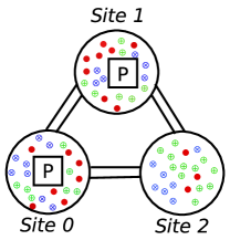
Figure 1: Protestors of different frames (colors) and police troops at two of three sites in the policing protest domain. The state space of police decision making is factored into the protest intensity levels at the sites.

Example 1 (Policing Protest)

Consider a policing scenario where police (agent $0$) must maintain order in 3 geographically distributed and designated protest sites (labeled 0, 1, and 2) as shown in Fig. 1. A population of $N$ agents are protesting at these sites. Police may dispatch one or two riot-control troops to either the same or different locations. Protests with differing intensities, low, medium and high (disruptive), occur at each of the three sites. The goal of the police is to deescalate protests to the low intensity at each site. Protest intensity at any site is influenced by the number of protestors and the number of police troops at that location. In the absence of adequate policing, we presume that the protest intensity escalates. On the other hand, two police troops at a location are adequate for de-escalating protests.

Factored Beliefs and Update

As we mentioned previously, the subject agent in an I-POMDP maintains a belief over the physical state and joint models of other agents, $b_{0,l}\in\Delta(S\times\prod_{j=1}^{N}M_{j,l-1})$, where $\Delta(\cdot)$ is the space of probability distributions. For settings such as Example 1 where $N$ is large, the size of the interactive state space is exponentially larger, $|IS_{0,l}|=|S||M_{j,l-1}|^{N}$, and the belief representation unwieldy. However, the representation becomes manageable for large $N$ if the belief is factored:

$$b_{0,l}(s,m_{1,l-1},m_{2,l-1},\ldots,m_{N,l-1})=Pr(s)~{}Pr(m_{1,l-1}|s)$$

$$\times Pr(m_{2,l-1}|s)\times\ldots\times Pr(m_{N,l-1}|s)$$ (1)

This factorization assumes conditional independence of models of different agents given the physical state. Consequently, beliefs that correlate agents may not be directly represented although correlation could be alternately supported by introducing models with a correlating device.

The memory consumed in storing a factored belief is $\mathcal{O}(|S|+N|S||M_{j}^{*}|)$, where $|M_{j}^{*}|$ is the size of the largest model space among all other agents. This is linear in the number of agents, which is much less than the exponentially growing memory required to represent the belief as a joint distribution over the interactive state space, $\mathcal{O}(|S||M_{j}^{*}|^{N})$.

Given agent 0’s belief at time $t$, $b_{0,l}^{t}$, its action $a_{0}^{t}$ and the subsequent observation it makes, $\omega_{0}^{t+1}$, the updated belief at time step $t+1$, $b_{0,l}^{t+1}$, may be obtained as:

$$Pr(s^{t+1},m_{1,l-1}^{t+1},\ldots,m_{N,l-1}^{t+1}|b_{0,l}^{t},a_{0}^{t},\omega_{0}^{t+1})=Pr(s^{t+1}|$$

$$b_{0,l}^{t},a_{0}^{t},\omega_{0}^{t+1})~{}Pr(m_{1,l-1}^{t+1}|s^{t+1},m_{2,l-1}^{t+1},\ldots,m_{N,l-1}^{t+1},$$

$$b_{0,l}^{t},a_{0}^{t},\omega_{0}^{t+1})\times\ldots\times Pr(m_{N,l-1}^{t+1}|s^{t+1},b_{0,l}^{t},a_{0}^{t},\omega_{0}^{t+1})$$ (2)

Each factor in the product of Eq. 2 may be obtained as follows. The update over the physical state is:

$$Pr(s^{t+1}|b_{0,l}^{t},a_{0}^{t},\omega_{0}^{t+1})\propto Pr(s^{t+1},\omega_{0}^{t+1}|b_{0,l}^{t},a_{0}^{t})$$

$$=\sum\limits_{s^{t}}b_{0,l}^{t}(s^{t})\sum\limits_{\mathbf{m}_{-0}^{t}}b_{0,l}^{t}(m_{1,l-1}^{t}|s^{t})\times\ldots\times b_{0,l}^{t}(m_{N,l-1}^{t}|s^{t})$$

$$\times\sum\limits_{\mathbf{a}_{-0}^{t}}Pr(a_{1}^{t}|m_{1,l-1}^{t})\times\ldots\times Pr(a_{N}^{t}|m_{N,l-1}^{t})$$

$$\times O_{0}^{t+1}(s^{t+1},\langle a_{0}^{t},\mathbf{a}_{-0}^{t}\rangle,\omega_{0}^{t+1})~{}T_{0}(s^{t},\langle a_{0}^{t},\mathbf{a}_{-0}^{t}\rangle,s^{t+1})$$ (3)

and the update over the model of each other agent, $j=1\ldots N$, conditioned on the state at $t+1$ is:

$$Pr(m_{j,l-1}^{t+1}|s^{t+1},m_{j+1,l-1}^{t+1},\ldots,m_{N,l-1}^{t+1},b_{0,l}^{t},a_{0}^{t},\omega_{0}^{t+1})=$$

$$\sum_{s^{t}}b_{0}^{t}(s^{t})\sum_{\mathbf{m}_{-j,l-1}^{t}}b_{0,l}^{t}(m_{1,l-1}^{t}|s^{t})\times\ldots\times b_{0,l}^{t}(m_{N,l-1}^{t}|s^{t})$$

$$\sum_{\mathbf{a}_{-j}^{t}}Pr(a_{1}^{t}|m_{1,l-1}^{t})\times\ldots\times Pr(a_{n}^{t}|m_{N,l-1}^{t})$$

$$\sum_{\omega_{j}^{t+1}}O_{j}(s^{t+1},\langle a_{j},\mathbf{a}_{-j}^{t}\rangle,\omega_{j}^{t+1})~{}Pr(m_{j}^{t+1}|m_{j}^{t},a_{j}^{t},\omega_{j}^{t+1})$$ (4)

Derivations of Eqs. 3 and 4 are straightforward and not given here due to lack of space. In particular, note that models of agents other than $j$ at $t+1$ do not impact $j$’s model update in the absence of correlated behavior. Thus, under the assumption of a factored prior as in Eq. 1 and absence of agent correlations, the I-POMDP belief update may be decomposed into an update of the physical state and update of the models of $N$ agents conditioned on the state.

Frame-Action Anonymity

As noted by Jiang et al. (?), many noncooperative and cooperative problems exhibit the structure that rewards depend on the number of agents acting in particular ways rather than which agent is performing the act. This is particularly evident in Example 1 where the outcome of policing largely depends on the number of protestors that are peaceful and the number that are disruptive. Building on this, we additionally observe that the transient state of the protests and observations of the police at a site are also largely influenced by the number of peaceful and disruptive protestors moving from one location to another. This is noted in the example below:

Example 2 (Frame-action anonymity of protestors)

The transient state of protests reflecting the intensity of protests at each site depends on the previous intensity at a site and the number of peaceful and disruptive protestors entering the site. Police (noisily) observes the intensity of protest at each site which is again largely determined by the number of peaceful and disruptive protestors at a site. Finally, the outcome of policing at a site is contingent on whether the protest is largely peaceful or disruptive. Consequently, the identity of the individual protestors beyond their frame and action is disregarded.

Here, peaceful and disruptive are different frames of others in agent 0’s I-POMDP, and the above definition may be extended to any number of frames. Frame-action anonymity is an important attribute of the above domain. We formally define it in the context of agent 0’s transition, observation and reward functions next:

Definition 1 (Frame-action anonymity)

Let $\mathbf{a}_{-0}^{p}$ be a joint action of all peaceful protestors and $\mathbf{a}_{-0}^{d}$ be a joint action of all disruptive ones. Let $\dot{\mathbf{a}}_{-0}^{p}$ and $\dot{\mathbf{a}}_{-0}^{d}$ be permutations of the two joint action profiles, respectively. An I-POMDP models frame-action anonymity iff for any $a_{0}$, $s$, $s^{\prime}$, $\mathbf{a}_{-0}^{p}$ and $\mathbf{a}_{-0}^{d}$:
$T_{0}(s$, $a_{0},\mathbf{a}_{-0}^{p},\mathbf{a}_{-0}^{d},s^{\prime})=T_{0}(s,a_{0},\dot{\mathbf{a}}_{-0}^{p},\dot{\mathbf{a}}_{-0}^{d},s^{\prime})$,
$O_{0}(s^{\prime},a_{0},\mathbf{a}_{-0}^{p},\mathbf{a}_{-0}^{d},\omega_{0})=O_{0}(s^{\prime},a_{0},\dot{\mathbf{a}}_{-0}^{p},\dot{\mathbf{a}}_{-0}^{d},\omega_{0})$, and
$R_{0}(s,a_{0},\mathbf{a}_{-0}^{p},\mathbf{a}_{-0}^{d})=R_{0}(s,a_{0},\dot{\mathbf{a}}_{-0}^{p},\dot{\mathbf{a}}_{-0}^{d})$   $\forall$ $\dot{\mathbf{a}}_{-0}^{p}$, $\dot{\mathbf{a}}_{-0}^{d}$.

Recall the definition of an action configuration, $\mathcal{C}$, as the vector of action counts of an agent population. A permutation of joint actions of others, say $\dot{\mathbf{a}}_{-0}^{p}$, assigns different actions to individual agents. Despite this, the fact that the transition and observation probabilities, and the reward remains unchanged indicates that the identity of the agent performing the action is irrelevant. Importantly, the configuration of the joint action and its permutation stays the same: $\mathcal{C}(\mathbf{a}_{-0}^{p})=\mathcal{C}(\dot{\mathbf{a}}_{-0}^{p})$. This combined with Def. 1 allows redefining the transition, observation and reward functions to be over configurations as: $T_{0}(s,a_{0},\mathcal{C}(\mathbf{a}_{-0}^{p}),\mathcal{C}(\mathbf{a}_{-0}^{d}),s^{\prime})$, $O_{0}(s^{\prime},a_{0},\mathcal{C}(\mathbf{a}_{-0}^{p}),\mathcal{C}(\mathbf{a}_{-0}^{d}),o)$ and $R_{0}(s,a_{0},\mathcal{C}(\mathbf{a}_{-0}^{p}),\mathcal{C}(\mathbf{a}_{-0}^{d}$ $))$.

Let $A_{1}^{p}$, …, $A_{n}^{p}$ be overlapping sets of actions of $n$ peaceful protestors, and $A_{-0}^{p}$ is the Cartesian product of these sets. Let $\mathcal{C}(A_{-0}^{p})$ be the set of all action configurations for $A_{-0}^{p}$. Observe that multiple joint actions from $A_{-0}^{p}$ may result in a single configuration; these joint actions are configuration equivalent. Consequently, the equivalence partitions the joint action set $A_{-0}^{p}$ into $|\mathcal{C}(A_{-0}^{p})|$ classes. Furthermore, when other agents of same frame have overlapping sets of actions, the number of configurations could be much smaller than the number of joint actions. Therefore, definitions of the transition, observation and reward functions involving configurations could be more compact.

Frame-Action Hypergraphs

In addition to frame-action anonymity, domains involving agent populations often exhibit context-specific independences. This is a broad category and includes the context-specific independence found in conditional probability tables of Bayesian networks (?) and in action-graph games. It offers significant additional structure for computational tractability. We begin by illustrating this in the context of Example 1.

Example 3 (Context-specific independence in policing)

At a low intensity protest site, reward for the police on passive policing is independent of the movement of the protestors to other sites. The transient intensity of the protest at a site given the level of policing at the site (context) is independent of the movement of protestors between other sites.

The context-specific independence above builds on the similar independence in action graphs in two ways: $(i)$ We model such partial independence in the transitions of factored states and in the observation function as well, in addition to the reward function. $(ii)$ We allow the context-specific independence to be mediated by the frames of other agents in addition to their actions. For example, the rewards received from policing a site is independent of the number of protestors at another site, instead the rewards are influenced by the number of peaceful and disruptive protestors present at that site.

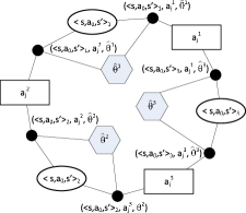
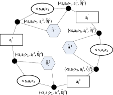
$(a)$                                      $(b)$

Figure 2: Levi (incidence) graph representation of a generic frame-action hypergraph for $(a)$ the transition function, and $(b)$ the reward function. The shaded nodes represent edges in the hypergraph. Each edge has the context, $\psi$, denoted in bold, agent’s action, $a$, and its frame, $\hat{\theta}$, incident on it. For example, the reward for a state and agent 0’s action, $\langle s,a_{0}\rangle_{1}$ is affected by others’ actions $a_{j}^{1}$ and $a_{j}^{2}$ performed by any other agent of frame $\hat{\theta}_{j}^{1}$ only.

The latter difference generalizes the action graphs into frame-action hypergraphs, and specifically 3-uniform hypergraphs where each edge is a set of 3 nodes. We formally define it below:

Definition 2 (Frame-action hypergraph)

A frame-action hypergraph for agent $0$ is a 3-uniform hypergraph $\mathcal{G}=\langle\Psi,A_{-0},\hat{\Theta}_{-0},E\rangle$, where $\Psi$ is a set of nodes that represent the context, $A_{-0}$ is a set of action nodes with each node representing an action that any other agent may take; $\hat{\Theta}_{-0}$ is a set of frame nodes, each node representing a frame ascribed to an agent, and $E$ is a 3-uniform hyperedge containing one node from each set $\Psi$, $A_{-0}$, and $\hat{\Theta}_{-0}$, respectively.

Both context and action nodes differ based on whether the hypergraph applies to the transition, observation or reward functions:

• For the transition function, the context is the set of all pairs of states between which a transition may occur and each action of agent $0$, $\Psi=S\times A_{0}\times S$, and the action nodes includes actions of all other agents, $A_{-0}$ $=$ $\bigcup_{j=1}^{N}A_{j}$. Neighbors of a context node $\psi$ $=$ $\langle s,a_{0},s^{\prime}\rangle$ are all the frame-action pairs that affect the probability of the transition. An edge $(\langle$ $s,a_{0},s^{\prime}\rangle$, $a_{-0}$, $\hat{\theta})$ indicates that the probability of transitioning from $s$ to $s^{\prime}$ on performing $a_{0}$ is affected (in part) by the other agents of frame $\hat{\theta}$ performing the particular action in $A_{-0}$.

• The context for agent $0$’s observation function is the state-action-observation triplet, $\Psi=S\times A_{0}\times\Omega_{0}$, and the action nodes are identical to those in the transition function. Neighbors of a context node, $\langle s,a_{0},\omega_{0}\rangle$, are all those frame-action pairs that affect the observation probability. Specifically, an edge $(\langle s,a_{0},\omega_{0}\rangle,a_{-0},\hat{\theta})$ indicates that the probability of observing $\omega_{0}$ from state $s$ on performing $a_{0}$ is affected (in part) by the other agents performing action, $a_{-0}$, who possess frame $\hat{\theta}$.

• For agent 0’s reward function, the context is the set of pairs of state and action of agent 0, $\Psi=S\times A_{0}$, and the action nodes the same as those in transition and observation functions. An edge $(\langle$ $s,a_{0}\rangle$, $a_{-0}$, $\hat{\theta}_{-0})$ in this hypergraph indicates that the reward for agent 0 on performing action $a_{0}$ at state $s$ is affected (in part) by the agents of frame $\hat{\theta}_{-0}$ who perform action in $A_{-0}$.

We illustrate a general frame-action hypergraph for context-specific independence in a transition function and a reward function as bipartite Levi graphs in Figs. 2$(a)$ and $(b)$, respectively. We point out that the hypergraph for the reward function comes closest in semantics to the graph in action graph games (?) although the former adds the state to the context and frames. Hypergraphs for the transition and observation functions differ substantially in semantics and form from action graphs.

To use these hypergraphs in our algorithms, we first define the general frame-action neighborhood of a context node.

Definition 3 (Frame-action neighborhood)

The frame-action neighborhood of a context node $\psi\in\Psi$, $\nu(\psi)$, given a frame-action hypergraph $\mathcal{G}$ is defined as a subset of $A\times\hat{\Theta}$ such that $\nu(\psi)=\{(a_{-0},\hat{\theta})|a_{-0}\in A_{-0},\hat{\theta}\in\hat{\Theta},(\psi,a_{-0},\hat{\theta})\in E\}$.

As an example, the frame-action neighborhood of a state-action pair, $\langle s,a_{0}\rangle$ in a hypergraph for the reward function is the set of all action and frame nodes incident on each hyperedge anchored by the node $\langle s,a_{0}\rangle$.

We move toward integrating frame-action anonymity introduced in the previous subsection with the context-specific independence as modeled above by introducing frame-action configurations.

Definition 4 (Frame-action configuration)

A configuration over the frame-action neighborhood of a context node, $\psi$, given a frame-action hypergraph is a vector,

$$\mathcal{C}^{\nu(\psi)}\overset{\triangle}{=}\langle~{}\mathcal{C}(A^{\hat{\theta}_{1}}_{-0}),\mathcal{C}(A^{\hat{\theta}_{2}}_{-0}),\ldots,\mathcal{C}(A^{\hat{\theta}_{|\hat{\Theta}|}}_{-0}),\mathcal{C}(\phi)~{}\rangle$$

where each $a$ included in $A^{\hat{\theta}}_{-0}$ is an action in $\nu(\psi)$ with frame $\hat{\theta}$, and $\mathcal{C}(A^{\hat{\theta}}_{-0})$ is a configuration over actions by agents other than 0 whose frame is $\hat{\theta}$. All agents with frames other than those in the frame-action neighborhood are assumed to perform a dummy action, $\phi$.

Definition 4 allows further inroads into compacting the transition, observation and rewards functions of the I-POMDP using context-specific independence. Specifically, we may redefine these functions one more time to limit the configurations only over the frame-action neighborhood of the context as, $T_{0}(s,a_{0},\mathcal{C}^{\nu(s,a_{0},s^{\prime})},s^{\prime})$, $O_{0}(s^{\prime},a_{0},\mathcal{C}^{\nu(s^{\prime},a_{0},\omega_{0})},\omega_{0})$ and $R_{0}(s,a_{0},\mathcal{C}^{\nu(s,a_{0})})$. 

Revised Framework

To benefit from structures of anonymity and context-specific independence, we redefine I-POMDP for agent $0$ as:

$$\text{{I-POMDP}{}}_{0,l}=\langle IS_{0,l},A,\Omega_{0},\mathcal{T}_{0},\mathcal{O}_{0},\mathcal{R}_{0},OC_{0}\rangle$$

where:

• $IS_{0,l}$, $A$, $\Omega_{0}$ and $OC_{0}$ remain the same as before. The physical states are factored as, $S=\prod_{k=1}^{K}X_{k}$.

• $\mathcal{T}_{0}$ is the transition function, $\mathcal{T}_{0}(x,a_{0},\mathcal{C}^{\nu(x,a_{0},x^{\prime})},x^{\prime})$ where $\mathcal{C}^{\nu(x,a_{0},x^{\prime})}$ is the configuration over the frame-action neighborhood of context $\langle x,a_{0},x^{\prime}\rangle$ obtained from a hypergraph that holds for the transition function. This transition function is significantly more compact than the original that occupies space $\mathcal{O}(|X|^{2}|A_{0}||A_{-0}|^{N})$ compared to the $\mathcal{O}(|X|^{2}|A_{0}|(\frac{N}{|\nu^{*}|})^{|\nu^{*}|})$ of $\mathcal{T}_{0}$, where the fraction is the complexity of $\binom{N+|\nu|^{*}+1}{|\nu^{*}|+1}$, $|\nu^{*}|$ is the maximum cardinality of the neighborhood of any context, and $(\frac{N}{|\nu^{*}|})^{|\nu^{*}|}$ $\ll$ $|A_{-0}|^{N}$. The value $\binom{N+|\nu|^{*}}{|\nu|^{*}}$ is obtained from combinatorial compositions and represents the number of ways $|\nu^{*}|+1$ non-negative values can be weakly composed such that their sum is $N$.

• The redefined observation function is $\mathcal{O}_{0}(x^{\prime},a_{0},\mathcal{C}^{\nu(x^{\prime},a_{0},\omega_{0})},\omega_{0})$ where $\mathcal{C}^{\nu(x^{\prime},a_{0},\omega_{0})}$ is the configuration over the frame-action neighborhood of context $\langle x^{\prime},a_{0},\omega_{0}\rangle$ obtained from a hypergraph that holds for the observation function. Analogously to the transition function, the original observation function consumes space $\mathcal{O}(|X||\Omega||A_{0}||A_{-0}|^{N})$, which is much larger than space $\mathcal{O}(|X||\Omega||A_{0}|(\frac{N}{|\nu^{*}|})^{|\nu^{*}|})$ occupied by this redefinition.

• $\mathcal{R}_{0}$ is the reward function defined as $\mathcal{R}_{0}(x,a_{0},\mathcal{C}^{\nu(x,a_{0})})$ where $\mathcal{C}^{\nu(x,a_{0})}$ is defined analogously to the configurations in the previous parameters. The reward for a state and actions may simply be the sum of rewards for the state factors and actions (or a more general function if needed). As with the transition and observation functions, this reward function is compact occupying space $\mathcal{O}(|X||A_{0}|(\frac{N}{|\nu^{*}|})^{|\nu^{*}|})$ that is much less than $\mathcal{O}(|X||A_{0}||A_{-0}|^{N})$ of the original.

Belief Update

For this extended I-POMDP, we compute the updated belief over a physical state as a product of its factors using Eq. 5 and belief update over the models of each other agent using Eq 6 as shown below:

$$Pr(\mathbf{s}^{t+1}|b_{0,l}^{t},a_{0}^{t},\omega_{0}^{t+1})\propto\bigg{\{}\sum\limits_{\mathbf{s}^{t}}b_{0,l}^{t}(\mathbf{s}^{t})\prod\limits_{k=1}^{K}\sum_{\mathcal{C}^{\nu(x_{k}^{t+1},a_{0}^{t},\omega_{0}^{t+1})}}$$

$$Pr(\mathcal{C}^{\nu(x_{k}^{t+1},a_{0}^{t},\omega_{0}^{t+1})}|b_{0,l}^{t}(M_{1,l-1}|\mathbf{s}^{t}),\ldots,b_{0,l}^{t}(M_{N,l-1}|\mathbf{s}^{t}))$$

$$\mathcal{O}_{0}(x_{k}^{t+1},a_{0}^{t},\mathcal{C}^{\nu(x_{k}^{t+1},a_{0}^{t},\omega_{0}^{t+1})},\omega_{0}^{t+1})\bigg{\}}\times\bigg{\{}\sum\limits_{\mathbf{s}^{t}}b_{0,l}^{t}(\mathbf{s}^{t})\prod\limits_{k=1}^{K}$$

$$\sum_{\mathcal{C}^{\nu(x_{k}^{t},a_{0}^{t},x_{k}^{t+1})}}Pr(\mathcal{C}^{\nu(x_{k}^{t},a_{0}^{t},x_{k}^{t+1})}|b_{0,l}^{t}(M_{1,l-1}|\mathbf{s}^{t}),\ldots,$$

$$b_{0,l}^{t}(M_{N,l-1}|\mathbf{s}^{t}))\mathcal{T}_{0}(x_{k}^{t},\mathcal{C}^{\nu(x_{k}^{t},a_{0}^{t},x_{k}^{t+1})},x_{k}^{t+1})\bigg{\}}$$ (5)

Here, the term, $Pr(\mathcal{C}^{\nu(x_{k}^{t+1},a_{0}^{t},\omega_{0}^{t+1})}|b_{0,l}^{t}(M_{1,l-1}|s^{t}),\ldots,$ $b_{0,l}^{t}(M_{N,l-1}|s^{t}))$, is the probability of a frame-action configuration (see Def. 4) that is context specific to the triplet, $\langle x^{t+1},a_{0},\omega^{t+1}\rangle$. It is computed from the factored beliefs over the models of all others. We discuss this computation in the next section. The second configuration term has an analogous meaning and is computed similarly.

The factored belief update over the models of each other agent, $j=1\ldots N$, conditioned on the state at $t+1$ becomes:

$$Pr(m_{j,l-1}^{t+1}|s^{t+1},\mathbf{m}_{-j,l-1}^{t+1},b_{0,l}^{t},a_{0}^{t})=\sum_{\mathbf{s}^{t}}b_{0}^{t}(\mathbf{s}^{t})\sum_{m_{j}^{t}}b_{0}^{t}(m_{j}^{t}$$

$$|s^{t})\sum_{a_{j}^{t}}Pr(a_{j}^{t}|m_{j}^{t})\sum_{\mathcal{C}^{\nu(x^{t+1},a_{j}^{t},\omega_{j})}}Pr(\mathcal{C}^{\nu(x^{t+1},a_{j}^{t},\omega_{j})}|$$

$$b_{0,l}^{t}(M_{1,l-1}|\mathbf{s}^{t}),\ldots,b_{0,l}^{t}(M_{N,l-1}|\mathbf{s}^{t}))\sum_{o_{j}^{t+1}}\mathcal{O}_{j}(x^{t+1},$$

$$a_{j}^{t},\mathcal{C}^{\nu(x^{t+1},a_{j}^{t},\omega_{j})},\omega_{j}^{t+1})~{}Pr(m_{j}^{t+1}|m_{j}^{t},a_{j}^{t},\omega_{j}^{t+1})$$ (6)

Proofs for obtaining Eqs. 5 and 6 are omitted due to space restrictions. Notice that the distributions over configurations are computed using distributions over other agents’ models. Therefore, we must maintain and update conditional beliefs over other agents’ models. Hence, the problem cannot be reduced to a POMDP by including configurations with physical states.

Value Function

The finite-horizon value function of the many-agent I-POMDP continues to be the sum of agent 0’s immediate reward and the discounted expected reward over the future:

$$V^{h}(m_{0,l}^{t})= \max_{a_{0}^{t}\in A_{0}}~{}ER_{0}(b_{0,l}^{t},a_{0}^{t})+$$

$$\gamma\sum\limits_{\omega_{0}^{t+1}}Pr(\omega_{0}^{t+1}|b_{0,l}^{t},a_{0}^{t})V^{h-1}(m_{0,l}^{t+1})$$ (7)

where $ER_{0}(b_{0,l}^{t},a_{0}^{t})$ is the expected immediate reward of agent $0$ and $\gamma$ is the discount factor. In the context of the redefined reward function of the many-agent I-POMDP framework in this section, the expected immediate reward is obtained as:

$$ER_{0}(b_{0,l}^{t},a_{0}^{t})=\sum_{\mathbf{s}^{t}}b_{0,l}^{t}(\mathbf{s}^{t})\bigg{(}\sum_{k=1}^{K}\sum_{\mathcal{C}^{\nu(x_{k}^{t},a_{0}^{t})}}Pr(\mathcal{C}^{\nu(x_{k}^{t},a_{0}^{t})}|$$

$$b_{0,l}^{t}(M_{1,l-1}|\mathbf{s}^{t}),\ldots,b_{0,l}^{t}(M_{N,l-1}|\mathbf{s}^{t}))R_{0}(x_{k}^{t},a_{0}^{t},\mathcal{C}^{\nu(x_{k}^{t},a_{0}^{t}})\bigg{)}$$ (8)

where the outermost sum is over all the state factors, $\mathbf{s}^{t}=\langle x_{1}^{t},\ldots,x_{K}^{t}\rangle$, and the term, $Pr(\mathcal{C}^{\nu(x_{k}^{t},a_{0}^{t})}|b_{0,l}^{t}(M_{1,l-1}|\mathbf{s}^{t}),\ldots,b_{0,l}^{t}(M_{N,l-1}|\mathbf{s}^{t}))$ denotes the probability of a frame-action configuration that is context-specific to the factor, $x_{k}^{t}$. Importantly, Proposition 1 establishes that the Bellman equation above is exact. The proof is given in the extended version of this paper (?).

Proposition 1 (Optimality)

The dynamic programming in Eq. 7 provides an exact computation of the value function for the many-agent I-POMDP.

Algorithms

We present an algorithm that computes the distribution over frame-action configurations and outline our simple method for solving the many-agent I-POMDP defined previously.

Distribution Over Frame-Action Configurations

Algorithm 1 generalizes an algorithm by Jiang and Lleyton-Brown (?) for computing configurations over actions given mixed strategies of other agents to include frames and conditional beliefs over models of other agents. It computes the probability distribution of configurations over the frame-action neighborhood of an action given the belief over the agents’ models: $Pr(\mathcal{C}^{\nu(x,a_{0},\omega_{0})}|b_{0,l}^{t}(M_{1,l-1}|\mathbf{s}^{t}),$ $\ldots,b_{0,l}^{t}(M_{N,l-1}|\mathbf{s}^{t}))$ and $Pr(\mathcal{C}^{\nu(x,a_{0},x^{\prime})}|b_{0,l}^{t}(M_{1,l-1}|\mathbf{s}^{t}),\ldots,$ $b_{0,l}^{t}(M_{N,l-1}|\mathbf{s}^{t}))$ in Eq. 5, $Pr(\mathcal{C}^{\nu(x,\omega_{j})}|b_{0,l}^{t}(M_{1,l-1}|\mathbf{s}^{t}),\ldots,$ $b_{0,l}^{t}(M_{N,l-1}|\mathbf{s}^{t}))$
in Eq. 6, and $Pr(\mathcal{C}^{\nu(x,a_{0})}|b_{0,l}^{t}(M_{1,l-1}|\mathbf{s}^{t}),\ldots,$ $b_{0,l}^{t}(M_{N,l-1}|\mathbf{s}^{t}))$ in Eq. 8.

Algorithm 1 Computing $Pr(\mathcal{C}^{\nu(\cdot)}|b_{0,l}(M_{1,l-1}|\mathbf{s}),$ $\ldots,b_{0,l}(M_{N,l-1}|\mathbf{s}))$

Input: $\nu(\cdot)$, $\langle b_{0,l}(M_{1,l-1}|\mathbf{s}),\ldots,b_{0,l}(M_{N,l-1}|\mathbf{s})\rangle$
Output: A trie $\mathcal{P}_{n}$ representing distribution over the frame-action configurations over $\nu(\cdot)$

1:  Initialize $c_{0}\leftarrow(0,\ldots,0)$, one value for each frame-action pair in $\nu(\cdot)$ and for $\phi$. Insert into empty trie $\mathcal{P}_{0}$

2:  Initialize $\mathcal{P}_{0}[c_{0}]\leftarrow 1$

3:  for $j\leftarrow 1$ to $N$ do

4:     Initialize $\mathcal{P}_{j}$ to be an empty trie

5:     for all $c_{j-1}$ from $\mathcal{P}_{j-1}$ do

6:        for all $m_{j,l-1}\in M_{j,l-1}$ do

7:           for all $a_{j}\in A_{j}$ such that $Pr(a_{j}|m_{j,l-1})>0$ do

8:              $c_{j}\leftarrow c_{j-1}$

9:              if $\langle a_{j},\hat{\theta}_{j}\rangle\in\nu(\cdot)$ then

10:                 $c_{j}[a_{j}]\leftarrow c_{j}[a_{j}]+1$

11:              else

12:                 $c_{j}[\phi]\leftarrow c_{j}[\phi]+1$

13:              if $\mathcal{P}_{j}[c_{j}]$ does not exist  then

14:                 Initialize $\mathcal{P}_{j}[c_{j}]\leftarrow 0$

15:              $\mathcal{P}_{j}[c_{j}]\leftarrow\mathcal{P}_{j}[c_{j}]+\mathcal{P}_{j-1}[c_{j-1}]\times Pr(a_{j}|m_{j,l-1})\times b_{0,l}(m_{j,l-1}|\mathbf{s})$

16:  return  $\mathcal{P}_{n}$

Algorithm 1 adds the actions of each agent one at a time. A Trie data structure enables efficient insertion and access of the configurations. We begin by initializing the configuration space for 0 agents ($\mathcal{P}_{0}$) to contain one tuple of integers ($c_{0}$) with $|\nu|+1$ 0s and assign its probability to be 1 (lines 1-2). Using the configurations of the previous step, we construct the configurations over the actions performed by $j$ agents by adding 1 to a relevant element depending on $j$’s action and frame (lines 3-15). If an action $a_{j}$ performed by $j$ with frame $\hat{m_{j}}$ is in the frame-action neighborhood $\nu(\cdot)$, then we increment its corresponding count by 1. Otherwise, it is considered as a dummy action and the count of $\phi$ is incremented (lines 9-12). Similarly, we update the probability of a configuration using the probability of $a_{j}$ and that of the base configuration $c_{j-1}$ (line 15). This algorithm is invoked multiple times for different values of $\nu(\cdot)$ as needed in the belief update and value function computation.

We utilize a simple method for solving the many-agent I-POMDP given an initial belief: each other agent is modeled using a finite-state controller as part of the interactive state space. A reachability tree of beliefs as nodes is projected for as many steps as the horizon (using Eqs. 5 and 6) and value iteration (Eq. 7) is performed on the tree. In order to mitigate the curse of history due to the branching factor that equals the number of agent 0’s actions and observations, we utilize the well-known technique of sampling observations from the propagated belief and obtain a sampled tree on which value iteration is run to get a policy. Action for any observation that does not appear in the sample is that which maximizes the immediate expected reward.

Computational Savings

The complexity of accessing an element in a ternary search trie is $\Theta(\nu)$. The maximum number of configurations encountered at any iteration is upper bounded by total number of configurations for $N$ agents, i.e. $\mathcal{O}((\frac{N}{|\nu^{*}|})^{|\nu^{*}|})$. The complexity of Algorithm 1 is polynomial in $N$, $\mathcal{O}(N|M_{j}^{*}||A_{j}^{*}||\nu^{*}|(\frac{N}{|\nu^{*}|})^{|\nu^{*}|})$ where $M_{j}^{*}$ and $A_{j}^{*}$ are largest sets of models and actions for any agent.

For the traditional I-POMDP belief update, the complexity of computing Eq. 3 is $\mathcal{O}(|S||M_{j}^{*}|^{N}|A_{j}^{*}|^{N})$ and that for computing Eq. 4 is $\mathcal{O}(|S||M_{j}^{*}|^{N}|A_{j}^{*}|^{N}|\Omega_{j}^{*}|)$ where ^∗ denotes the maximum cardinality of a set for any agent. For a factored representation, belief update operator invokes Eq. 3 for each value of all state factors and it invokes Eq. 4 for each model of each agent $j$ and for all values of updated states. Hence the total complexity of belief update is $\mathcal{O}(N|M_{j}^{*}||S|^{2}|M_{j}^{*}|^{N}|A_{j}^{*}|^{N}|\Omega_{j}^{*}|)$. The complexity of computing updated belief over state factor $x^{t+1}$ using Eq. 5 is $\mathcal{O}(|S|NK|M_{j}^{*}||A_{j}^{*}||\nu^{*}|(\frac{N}{|\nu^{*}|})^{|\nu^{*}|})$ (recall the complexity of Algorithm 1). Similarly, the complexity of computing updated model probability using Eq. 6 is $\mathcal{O}((|S|N|M_{j}^{*}||A_{j}^{*}||\nu^{*}|+|\Omega_{j}^{*}|)(\frac{N}{|\nu^{*}|})^{|\nu^{*}|})$. These complexity terms are polynomial in $N$ for small values of $|\nu^{*}|$ as opposed to exponential in $N$ as in Eqs. 3 and 4. The overall complexity of belief update is also polynomial in $N$.

Complexity of computing the immediate expected reward in the absence of problem structure is $\mathcal{O}(|S|K|M_{j}^{*}|^{N}|A_{j}^{*}|^{N})$. On the other hand, the complexity of computing expected reward using Eq. 8 is $\mathcal{O}(|S|KN|M_{j}^{*}||A_{j}^{*}||\nu^{*}|(\frac{N}{|\nu^{*}|})^{|\nu^{*}|})$, which is again polynomial in $N$ for low values of $|\nu^{*}|$. These complexities are discussed in greater detail in (?).

Experiments

We implemented a simple and systematic I-POMDP solving technique that computes reachable beliefs over the finite horizon and then calculates the optimal value at the root node using the Bellman equation for the Many-Agents I-POMDP framework. We evaluate its performance in the aforementioned non-cooperative policing protest scenario ($|S|=27,|A_{0}|=9,|A_{j}|=4,|O_{j}|=8,|O_{i}|=8$). We model the other agents as POMDPs and solve them using bounded policy iteration (?), representing the models as finite state controllers. This representation enables us to have a compact model space. We set the maximum planning horizon to 4 throughout the experiments. The frame-action hypergraphs are encoded into the transition, observation and reward functions of the Many-Agent I-POMDP (Fig. 3). All computations are carried out on a RHEL platform with 2.80 GHz processor and 4 GB memory.

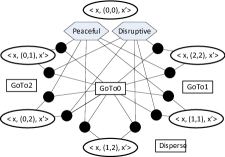
$(a)$                                      $(b)$

Figure 3: A compact Levi graph representation of policing protest as a frame-action hypergraph for $(a)$ the transition function, and $(b)$ the reward function at site 0. Variables $x$ and $x^{\prime}$ represent the start and end intensities of the protest at site 0 and the action shows the location of the two police troops. As two police troops are sufficient to de-escalate any protest, the contexts in which both troops are at site 0 are independent of the actions of other agents. All other contexts depend on the agents choosing to protest at site 0 only.

To evaluate the computational gain obtained by exploiting problem structures, we implemented a solution algorithm similar to the one described earlier that does not exploit any problem structure. A comparison of the Many-Agent I-POMDP with the original I-POMDP yields two important results: ($i$) When there are few other agents, the Many-Agent I-POMDP provides exactly the same solution as the original I-POMDP but with reduced running times by exploiting the problem structure. ($ii$) Many-Agent I-POMDP scales to larger agent populations, from 100 to 1,000+, and the new framework delivers promising results within reasonable time.

Protestors	H	I-POMDP	Many-Agent	Exp. Value
2	2	1 s	0.55 s	77.42
	3	19 s	17 s	222.42
3	2	3 s	0.56 s	77.34
	3	38 s	17 s	222.32
4	2	39 s	0.57 s	76.96
	3	223 s	17 s	221.87
5	2	603 s	0.60 s	76.88
	3	2,480 s	18 s	221.77

Table 1: Comparison between traditional I-POMDP and Many-Agent I-POMDP both following same solution approach of computing a reachability tree and performing backup.

In the first setting, we consider up to 5 protestors with different frames. As shown in Table 1, both the traditional and the Many-Agent I-POMDP produce policies with the same expected value. However, as the Many-Agent I-POMDP losslessly projects joint actions to configurations, it requires much less running time.

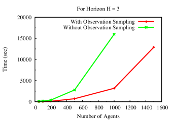
$(a)$

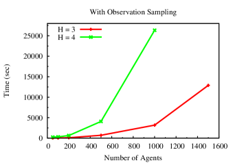
$(b)$

Figure 4: $(a)$ The computational gain obtained by observation sampling. $(b)$ Performance of Many-Agent I-POMDP with observation sampling for horizon 3 and 4. The time required to solve a problem is polynomial in the number of agents.

Our second setting considers a large number of protestors, for which the traditional I-POMDP does not scale. Instead, we first scale up the exact solution method using Many-Agent I-POMDP to deal with a few hundreds of other agents. Although the exploitation of the problem structures reduces the curse of dimensionality that plagues I-POMDPs, the curse of history is unaffected by such approaches. To mitigate the curse of history we use the well-known observation sampling method (?), which allows us to scale to over 1,000 agents in a reasonable time of 4.5 hours as we show in Fig. 4$(a)$. This increases to about 7 hours if we extend the horizon to 4 as shown in Fig. 4$(b)$.

Conclusion

The key contribution of the Many-Agent I-POMDP is its scalability beyond 1,000 agents by exploiting problem structures. We formalize widely existing problem structures – frame-action anonymity and context-specific independence – and encode it as frame-action hypergraphs. Other real-world examples exhibiting such problem structure are found in economics where the value of an asset depends on the number of agents vying to acquire it and their financial standing (frame), in real estate where the value of a property depends on its demand, the valuations of neighboring properties as well as the economic status of the neighbors because an upscale neighborhood is desirable. Compared to the previous best approach (?), which scales to an extension of the simple tiger problem involving 5 agents only, the presented framework is far more scalable in terms of number of agents. Our future work includes exploring other types of problem structures and developing approximation algorithms for this I-POMDP. An integration with existing multiagent simulation platforms to illustrate the behavior of agent populations may be interesting.

Appendix

Factored Belief Update:

$$b_{0,l}(s^{t+1},m_{1}^{t+1},\ldots,m_{n}^{t+1})$$

$$=Pr(s^{t+1},m_{1}^{t+1},\ldots,m_{n}^{t+1}|b_{0}^{t},a_{0}^{t},\omega_{0}^{t+1})$$

$$=Pr(s^{t+1}|b_{0}^{t},a_{0}^{t},\omega_{0}^{t+1})\times Pr(m_{1}^{t+1}|s^{t+1},b_{0}^{t},a_{0}^{t},\omega_{0}^{t+1})$$

$$~{}~{}~{}\times\cdots\times Pr(m_{n}^{t+1}|s^{t+1},m_{1}^{t+1},\ldots,m_{n-1}^{t+1}b_{0}^{t},a_{0}^{t},\omega_{0}^{t+1})$$

Derivation of equation 5:
Starting with equation 3, we have:

$$Pr(s^{t+1}|b_{0,l}^{t},a_{0}^{t},\omega_{0}^{t+1})\propto Pr(s^{t+1},\omega_{0}^{t+1}|b_{0,l}^{t},a_{0}^{t})$$

$$=Pr(s^{t+1}|b_{0,l}^{t},a_{0}^{t})Pr(\omega_{0}^{t+1}|s^{t+1},b_{0,l}^{t},a_{0}^{t})$$

The update term for physical states may be represented as a product of its factors such that for any factor $X_{k}$:

$$Pr(x_{k}^{t+1}|b_{0,l}^{t},a_{0}^{t})=\sum\limits_{s^{t}}b_{0,l}^{t}(s^{t})\sum\limits_{\mathbf{m}_{-0}^{t}}b_{0,l}^{t}(\mathbf{m}_{-0}^{t}|s^{t})\times$$

$$\sum\limits_{\mathbf{a}_{-0}^{t}}Pr(\mathbf{a}_{-0}^{t}|\mathbf{m}_{-0}^{t})~{}T_{0}(x_{k}^{t},\langle a_{0}^{t},\mathbf{a}_{-0}^{t}\rangle,x_{k}^{t+1})$$

where $b_{0,l}^{t}(\mathbf{m}_{-0}^{t}|s^{t})=b_{0,l}^{t}(m_{1}^{t}|s^{t})\times\ldots\times b_{0,l}^{t}(m_{N}^{t}|s^{t})$, and $Pr(\mathbf{a}_{-0}^{t}|\mathbf{m}_{-0}^{t})=Pr(a_{1}^{t}|m_{1}^{t})\times\ldots\times Pr(a_{N}^{t}|m_{N}^{t})$.

We introduce a projection function $\delta^{\nu(\psi)}$ that maps joint actions to the corresponding frame-action configurations as defined in definition 4. Formally $\delta^{\nu(\psi)}:\mathbf{a}\rightarrow\mathbf{C}^{\nu(\psi)}$, where $\mathbf{C}^{\nu(\psi)}$ is the set of all possible configurations such that for all agents $j$ with frame $\hat{\theta}$, $\mathcal{C}(a,\hat{\theta})=|\{j:a_{j}=a,\hat{\theta}_{j}=\hat{\theta},(a_{j},\hat{\theta})\in\nu(\psi)\}|$.

Next we partition the set of joint action of all other agents $\bf{A}_{-0}$ into smaller subsets $\bf{A}_{-0}^{1},~{}\ldots,~{}\bf{A}_{-0}^{|\mathbf{C}^{\nu(\psi)}|}$ such that the projection function $\delta^{\nu(\psi)}$ maps all joint actions belonging to any given partition $\bf{A}_{-0}^{c}$ to the same value configuration. Hence, we may rewrite the above equation as:

$$Pr(x_{k}^{t+1}|b_{0,l}^{t},a_{0}^{t})=\sum\limits_{s^{t}}b_{0,l}^{t}(s^{t})\sum\limits_{c=1}^{|\mathbf{C}^{\nu(x_{k}^{t},a_{0}^{t},x_{k}^{t+1})}|}\sum\limits_{\mathbf{m}_{-0}^{t}}$$

$$b_{0,l}^{t}(\mathbf{m}_{-0}^{t}|s^{t})\sum\limits_{\mathbf{a}_{-0}^{t}\in\bf{A}_{-0}^{c}}Pr(\mathbf{a}_{-0}^{t}|\mathbf{m}_{-0}^{t})$$

$$~{}T_{0}(x_{k}^{t},\langle a_{0}^{t},\mathbf{a}_{-0}^{t}\rangle,x_{k}^{t+1})$$

Under frame-action anonymity and frame-action independence, for all joint actions $\mathbf{a}_{-0}^{t}\in\bf{A}_{-0}^{c}$ $T_{0}(x_{k}^{t},\langle a_{0}^{t},\mathbf{a}_{-0}^{t}\rangle,x_{k}^{t+1})$ $=$ $T_{0}(x_{k}^{t},a_{0}^{t},\mathcal{C}^{\nu(x^{t},a_{0}^{t},x^{t+1})},x_{k}^{t+1})$, where $\mathcal{C}^{\nu(x_{k}^{t},a_{0}^{t},x_{k}^{t+1})}$ $=$ $\delta^{\nu(x_{k}^{t},a_{0}^{t},x_{k}^{t+1})}(\mathbf{a}_{-0}^{t})$.

$$Pr(x_{k}^{t+1}|b_{0,l}^{t},a_{0}^{t})=\sum\limits_{s^{t}}b_{0,l}^{t}(s^{t})\sum\limits_{c=1}^{|\mathbf{C}^{\nu(x_{k}^{t},a_{0}^{t},x_{k}^{t+1})}|}\sum\limits_{\mathbf{m}_{-0}^{t}}$$

$$b_{0,l}^{t}(\mathbf{m}_{-0}^{t}|s^{t})\sum\limits_{\mathbf{a}_{-0}^{t}\in\bf{A}_{-0}^{c}}Pr(\mathbf{a}_{-0}^{t}|\mathbf{m}_{-0}^{t})$$

$$T_{0}(x_{k}^{t},a_{0}^{t},\mathcal{C}^{\nu(x_{k}^{t},a_{0}^{t},x_{k}^{t+1})},x_{k}^{t+1})$$

The cumulative probability of joint actions mapping to the same configuration, $\sum\limits_{\mathbf{m}_{-0}^{t}}b_{0,l}^{t}(\mathbf{m}_{-0}^{t}|s^{t})$ $\sum\limits_{\mathbf{a}_{-0}^{t}\in\bf{A}_{-0}^{c}}Pr(\mathbf{a}_{-0}^{t}|\mathbf{m}_{-0}^{t})$, is computed tractably using algorithm 1 as $Pr(\mathcal{C}^{\nu(x_{k}^{t},a_{0}^{t},x_{k}^{t+1})}|b_{0,l}(M_{1}^{t}|s^{t}),\ldots b_{0,l}(M_{n}^{t}|s^{t}))$. Hence, the equation becomes:

$$Pr(x_{k}^{t+1}|b_{0,l}^{t},a_{0}^{t})=\sum\limits_{s^{t}}b_{0,l}^{t}(s^{t})\sum\limits_{\mathcal{C}^{\nu(x_{k}^{t},a_{0}^{t},x_{k}^{t+1})}}Pr(\mathcal{C}^{\nu(x_{k}^{t},a_{0}^{t},x_{k}^{t+1})}|$$

$$b_{0,l}(M_{1}^{t}|s^{t}),\ldots b_{0,l}(M_{n}^{t}|s^{t}))~{}\times~{}T_{0}(x^{t},a_{0}^{t},\mathcal{C}^{\nu(x_{k}^{t},a_{0}^{t},x_{k}^{t+1})},x^{t+1})$$

Similarly, the observation probability may also be obtained in a factored form and $\mathcal{C}^{\nu(s^{t+1},a_{0}^{t},\omega_{0}^{t+1})}=\delta^{\nu(s^{t+1},a_{0}^{t},\omega_{0}^{t+1})}(\mathbf{a}_{-0}^{t})$ may be substitued instead of the joint action.

$$Pr(\omega_{0}^{t+1}|s^{t+1},b_{0,l}^{t},a_{0}^{t})=\sum\limits_{\mathbf{s}^{t}}b_{0,l}^{t}(\mathbf{s}^{t})\prod\limits_{k=1}^{K}\sum_{\mathcal{C}^{\nu(x_{k}^{t+1},a_{0}^{t},\omega_{0}^{t+1})}}$$

$$Pr(\mathcal{C}^{\nu(x_{k}^{t+1},a_{0}^{t},\omega_{0}^{t+1})}|b_{0,l}^{t}(M_{1,l-1}|\mathbf{s}^{t}),\ldots,b_{0,l}^{t}(M_{N,l-1}|\mathbf{s}^{t}))$$

$$\mathcal{O}_{0}(x_{k}^{t+1},a_{0}^{t},\mathcal{C}^{\nu(x_{k}^{t+1},a_{0}^{t},\omega_{0}^{t+1})},\omega_{0}^{t+1})$$

Therefore, we may rewrite equation 3 as follows:

$$Pr(s^{t+1}|b_{0,l}^{t},a_{0}^{t},\omega_{0}^{t+1})\propto\bigg{\{}\sum\limits_{\mathbf{s}^{t}}b_{0,l}^{t}(\mathbf{s}^{t})\prod\limits_{k=1}^{K}\sum_{\mathcal{C}^{\nu(x_{k}^{t+1},a_{0}^{t},\omega_{0}^{t+1})}}$$

$$Pr(\mathcal{C}^{\nu(x_{k}^{t+1},a_{0}^{t},\omega_{0}^{t+1})}|b_{0,l}^{t}(M_{1,l-1}|\mathbf{s}^{t}),\ldots,b_{0,l}^{t}(M_{N,l-1}|\mathbf{s}^{t}))$$

$$\mathcal{O}_{0}(x_{k}^{t+1},a_{0}^{t},\mathcal{C}^{\nu(x_{k}^{t+1},a_{0}^{t},\omega_{0}^{t+1})},\omega_{0}^{t+1})\bigg{\}}\times\bigg{\{}\sum\limits_{\mathbf{s}^{t}}b_{0,l}^{t}(\mathbf{s}^{t})\prod\limits_{k=1}^{K}$$

$$\sum_{\mathcal{C}^{\nu(x_{k}^{t},a_{0}^{t},x_{k}^{t+1})}}Pr(\mathcal{C}^{\nu(x_{k}^{t},a_{0}^{t},x_{k}^{t+1})}|b_{0,l}^{t}(M_{1,l-1}|\mathbf{s}^{t}),\ldots,$$

$$b_{0,l}^{t}(M_{N,l-1}|\mathbf{s}^{t}))\mathcal{T}_{0}(x_{k}^{t},\mathcal{C}^{\nu(x_{k}^{t},a_{0}^{t},x_{k}^{t+1})},x_{k}^{t+1})\bigg{\}}$$ (9)

Derivation of equation 6:
The belief update over the models of agent $j$ shown in equation 4 can be rewritten as follows:

$$Pr(m_{j,l-1}^{t+1}|s^{t+1},m_{j+1,l-1}^{t+1},\ldots,m_{N,l-1}^{t+1},b_{0,l}^{t},a_{0}^{t},\omega_{0}^{t+1})$$

$$=\sum_{s^{t}}b_{0}^{t}(s^{t})\sum_{\mathbf{m}_{1,l-1}^{t}}b_{0,l}^{t}(m_{1,l-1}^{t}|s^{t})\sum_{a_{1}^{t}}Pr(a_{1}^{t}|m_{1,l-1}^{t})$$

$$\ldots\sum_{\mathbf{m}_{j-1,l-1}^{t}}b_{0,l}^{t}(m_{j-1,l-1}^{t}|s^{t})\sum_{a_{j-1}^{t}}Pr(a_{j-1}^{t}|m_{j-1,l-1}^{t})$$

$$\sum_{\mathbf{m}_{j,l-1}^{t}}b_{0,l}^{t}(m_{j,l-1}^{t}|s^{t})\sum_{a_{j}^{t}}Pr(a_{j}^{t}|m_{j,l-1}^{t})\sum_{\mathbf{m}_{j+1,l-1}^{t}}$$

$$b_{0,l}^{t}(m_{j+1,l-1}^{t}|s^{t})\sum_{a_{j+1}^{t}}Pr(a_{j+1}^{t}|m_{j,l-1}^{t})~{}\ldots~{}\sum_{\mathbf{m}_{N,l-1}^{t}}$$

$$b_{0,l}^{t}(m_{N,l-1}^{t}|s^{t})\sum_{a_{N}^{t}}Pr(a_{N}^{t}|m_{N,l-1}^{t})\sum_{\omega_{j}^{t+1}}$$

$$O_{j}(s^{t+1},\langle a_{j},\mathbf{a}_{-j}^{t}\rangle,\omega_{j}^{t+1})~{}Pr(m_{j}^{t+1}|m_{j}^{t},a_{j}^{t},\omega_{j}^{t+1})$$

Substituting frame-action configuration as in equation 9, we get:

$$Pr(m_{j,l-1}^{t+1}|s^{t+1},m_{j+1,l-1}^{t+1},\ldots,m_{N,l-1}^{t+1},b_{0,l}^{t},a_{0}^{t},\omega_{0}^{t+1})$$

$$=\sum_{\mathbf{s}^{t}}b_{0}^{t}(\mathbf{s}^{t})\sum_{m_{j}^{t}}b_{0}^{t}(m_{j}^{t}|s^{t})\sum_{a_{j}^{t}}Pr(a_{j}^{t}|m_{j}^{t})\sum_{\mathcal{C}^{\nu(x^{t+1},a_{j}^{t},\omega_{j})}}$$

$$Pr(\mathcal{C}^{\nu(x^{t+1},a_{j}^{t},\omega_{j})}|a_{0}^{t},b_{0,l}^{t}(M_{1}|\mathbf{s}^{t}),\ldots,b_{0,l}^{t}(M_{j-1}|\mathbf{s}^{t}),$$

$$b_{0,l}^{t}(M_{j+1}|\mathbf{s}^{t}),\ldots b_{0,l}^{t}(m_{N}|\mathbf{s}^{t}))\times\sum_{o_{j}^{t+1}}\mathcal{O}_{j}(x^{t+1},a_{j}^{t},$$

$$\mathcal{C}^{\nu(x^{t+1},\omega_{j})},\omega_{j}^{t+1})~{}Pr(m_{j}^{t+1}|m_{j}^{t},a_{j}^{t},\omega_{j}^{t+1})$$ (10)

Where the probability over the configurations is computed as in algorithm 1 using belief over models of all other agents except $j$. In the end we add 1 to the count of action $a_{0}$ in every configuration.

Complexity of belief update:
For the traditional I-POMDP belief update, the complexity of computing equation 3 is $\mathcal{O}(|S|(|M_{j}^{*}|)^{N}(|A_{j}^{*}|)^{N})$ and that for computing equation 4 is $\mathcal{O}(|S||M_{j}^{*}|^{N}|A_{j}^{*}|^{N}|\Omega_{j}^{*}|)$ where ^∗ denotes the maximum cardianlity of a set for any agent. For factored representation, belief update operator invokes equation 3 for each value of all state factors and it invokes equation 4 for each model of each agent $j$ and for all values of updated states. Hence the total complexity of belief update is $\mathcal{O}(K|X^{*}||S||M_{j}^{*}|^{N}|A_{j}^{*}|^{N}$ $+N|M_{j}^{*}||S|^{2}(|M_{j}^{*}|)^{N}|A_{j}^{*}|^{N}|\Omega_{j}^{*}|)$.

In equation 5, algorithm is called once for all values of $\mathbf{s}^{t}$. The two inner summations iterate over all possible configurations over transition and observation contexts. The number of configurations is upper bounded by $\binom{N+|\nu^{*}|}{|\nu^{*}|}$ where $|\nu^{*}|$ is the maximum cardinality of the frame-action neighborhood for any context. Hence the complexity of computing updated belief of state factor $x^{t+1}$ using equation 5 is $\mathcal{O}(|S|K\times\{N|M_{j}^{*}||A_{j}^{*}||\nu^{*}|\binom{N+|\nu^{*}|}{|\nu^{*}|}$ $+\binom{N+|\nu^{*}|}{|\nu^{*}|}\})$ (recall the complexity of algorithm 1). Similarly, the complexity of computing updated model probability using equation 6 is $\mathcal{O}(|S|\times\{N|M_{j}^{*}||A_{j}^{*}||\nu^{*}|\binom{N+|\nu^{*}|}{|\nu^{*}|}+|\Omega_{j}^{*}|$ $\binom{N+|\nu^{*}|}{|\nu^{*}|}\})$. These complexity terms are polynomial in $N$ for small values of $|\nu^{*}|$ as opposed to exponential in $N$ as in equations 3 and 4. The overall complexity of belief update is also polynomial in $N$.

Proof of Proposition 1:
The expected reward of agent $0$ is obtained as the sum of reward factors.

$$ER_{0}(b_{0,l}^{t},a_{0}^{t})=\sum_{\mathbf{s}^{t}}b_{0,l}^{t}(s^{t})\bigg{(}\sum_{k=1}^{K}\sum_{\mathbf{m}_{-0}^{t}}b_{0,l}^{t}(m_{1}^{t}|s^{t})\times\ldots\times$$

$$b_{0,l}^{t}(m_{N}^{t}|s^{t})\times\sum\limits_{\mathbf{a}_{-0}^{t}}Pr(a_{1}^{t}|m_{1,l-1}^{t})\times\ldots\times Pr(a_{N}^{t}|m_{N,l-1}^{t})$$

$$R_{0}(x_{k}^{t},\langle a_{0}^{t},\mathbf{a}_{-0}^{t}\rangle)\bigg{)}$$

Complexity of computing expected reward using the above equation is $\mathcal{O}(|S|K(|M_{j}^{*}|)^{N}(|A_{j}^{*}|)^{N})$. Equation 8 is derived similarly to the belief update by substituting distribution over frame-action configurations for distributions over joint models and joint actions. This combined with the proofs for Eqs. 5 and 6 allow us to obtain Eq.7 from the Bellman equation of the original I-POMDP.

The complexity of computing expected reward using equation 8 is
$\mathcal{O}(|S|K\{N|M_{j}^{*}||A_{j}^{*}||\nu^{*}|+1\}\binom{N+|\nu^{*}|}{|\nu^{*}|})$ which is again polynomial in $N$ for low values of $|\nu^{*}|$.

References

• [Boutilier et al. 1996] Boutilier, C.; Friedman, N.; Goldszmidt, M.; and Koller, D. 1996. Context-specific independence in bayesian networks. In Twelfth international conference on Uncertainty in artificial intelligence (UAI), 115–123.
• [Chandrasekaran et al. 2014] Chandrasekaran, M.; Doshi, P.; Zeng, Y.; and Chen, Y. 2014. Team behavior in interactive dynamic influence diagrams with applications to ad hoc teams (extended abstract). In Autonomous Agents and Multi-Agent Systems Conference (AAMAS), 1559–1560.
• [Doshi and Gmytrasiewicz 2009] Doshi, P., and Gmytrasiewicz, P. J. 2009. Monte Carlo sampling methods for approximating interactive POMDPs. Journal of Artificial Intelligence Research 34:297–337.
• [Doshi and Perez 2008] Doshi, P., and Perez, D. 2008. Generalized point based value iteration for interactive POMDPs. In Twenty Third Conference on Artificial Intelligence (AAAI), 63–68.
• [Doshi et al. 2010] Doshi, P.; Qu, X.; Goodie, A.; and Young, D. 2010. Modeling recursive reasoning in humans using empirically informed interactive POMDPs. In International Autonomous Agents and Multiagent Systems Conference (AAMAS), 1223–1230.
• [Doshi 2012] Doshi, P. 2012. Decision making in complex multiagent settings: A tale of two frameworks. AI Magazine 33(4):82–95.
• [Gmytrasiewicz and Doshi 2005] Gmytrasiewicz, P. J., and Doshi, P. 2005. A framework for sequential planning in multiagent settings. Journal of Artificial Intelligence Research 24:49–79.
• [Hoang and Low 2013] Hoang, T. N., and Low, K. H. 2013. Interactive POMDP lite: Towards practical planning to predict and exploit intentions for interacting with self-interested agents. In International Joint Conference on Artificial Intelligence (IJCAI), 2298–2305.
• [Jiang and Leyton-Brown 2010] Jiang, A. X., and Leyton-Brown, K. 2010. Bayesian action-graph games. In Advances in Neural Information Processing Systems (NIPS), 991–999.
• [Jiang, Leyton-Brown, and Bhat 2011] Jiang, A. X.; Leyton-Brown, K.; and Bhat, N. A. 2011. Action-graph games. Games and Economic Behavior 71(1):141–173.
• [Jiang, Leyton-Brown, and Pfeffer 2009] Jiang, A. X.; Leyton-Brown, K.; and Pfeffer, A. 2009. Temporal action-graph games: A new representation for dynamic games. In Twenty-Fifth Conference on Uncertainty in Artificial Intelligence (UAI), 268–276.
• [Kearns, Littman, and Singh 2001] Kearns, M.; Littman, M.; and Singh, S. 2001. Graphical models for game theory. In Uncertainty in Artificial Intelligence (UAI), 253–260.
• [Koller and Milch 2001] Koller, D., and Milch, B. 2001. Multi-agent influence diagrams for representing and solving games. In IJCAI, 1027–1034.
• [Nair et al. 2005] Nair, R.; Varakantham, P.; Tambe, M.; and Yokoo, M. 2005. Networked distributed POMDPs: A synthesis of distributed constraint optimization and POMDPs. In Twentieth AAAI Conference on Artificial Intelligence, 133–139.
• [Ng et al. 2010] Ng, B.; Meyers, C.; Boakye, K.; and Nitao, J. 2010. Towards applying interactive POMDPs to real-world adversary modeling. In Innovative Applications in Artificial Intelligence (IAAI), 1814–1820.
• [Poupart and Boutilier 2003] Poupart, P., and Boutilier, C. 2003. Bounded finite state controllers. In Neural Information Processing Systems.
• [Roughgarden and Tardos 2002] Roughgarden, T., and Tardos, E. 2002. How bad is selfish routing? Journal of ACM 49(2):236–259.
• [Seuken and Zilberstein 2008] Seuken, S., and Zilberstein, S. 2008. Formal models and algorithms for decentralized decision making under uncertainty. Journal of Autonomous Agents and Multiagent Systems 17(2):190–250.
• [Seymour and Peterson 2009] Seymour, R., and Peterson, G. L. 2009. A trust-based multiagent system. In IEEE International Conference on Computational Science and Engineering, 109–116.
• [Sonu and Doshi 2014] Sonu, E., and Doshi, P. 2014. Scalable solutions of interactive POMDPs using generalized and bounded policy iteration. Journal of Autonomous Agents and Multi-Agent Systems DOI: 10.1007/s10458–014–9261–5, in press.
• [Sonu, Chen, and Doshi 2015] Sonu, E.; Chen, Y.; and Doshi, P. 2015. Individual planning in agent populations: Exploiting anonymity and frame-action hypergraphs. Technical Report http://arxiv.org/abs/1503.07220, arXiv.
• [Varakantham, Adulyasak, and Jaillet 2014] Varakantham, P.; Adulyasak, Y.; and Jaillet, P. 2014. Decentralized stochastic planning with anonymity in interactions. In AAAI Conference on Artificial Intelligence, 2505–2511.
• [Varakantham et al. 2012] Varakantham, P.; Cheng, S.; Gordon, G.; and Ahmed, A. 2012. Decision support for agent populations in uncertain and congested environments. In Uncertainty in artificial intelligence (UAI), 1471–1477.
• [Wang 2013] Wang, F. 2013. An I-POMDP based multi-agent architecture for dialogue tutoring. In International Conference on Advanced ICT and Education (ICAICTE-13), 486–489.
• [Woodward and Wood 2012] Woodward, M. P., and Wood, R. J. 2012. Learning from humans as an i-pomdp. CoRR abs/1204.0274.
• [Wunder et al. 2011] Wunder, M.; Kaisers, M.; Yaros, J.; and Littman, M. 2011. Using iterated reasoning to predict opponent strategies. In International Conference on Autonomous Agents and Multi-Agent Systems (AAMAS), 593–600.