Excitation Gap of Fractal Quantum Hall States in Graphene

Abstract

In the presence of a magnetic field and an external periodic potential, the Landau level spectrum of a two-dimensional electron gas exhibits a fractal pattern in the energy spectrum which is described as the Hofstadter’s butterfly. In this work, we develop a Hartree-Fock theory to deal with the electron-electron interaction in the Hofstadter’s butterfly state in a finite-size graphene with periodic boundary conditions, in which we include both spin and valley degrees of freedom. We then treat the butterfly state as an electron crystal so that we could obtain the order parameters of the crystal in the momentum space and also in an infinite sample. The excitation gaps obtained in the infinite sample is comparable to those in the finite-size study, and agree with a recent experimental observation.

In a strong perpendicular magnetic field, the energy spectrum of a two-dimensional electron gas (2DEG) splits into a series of Landau levels. If a periodic potential is also added to this system, the noninteracting energy spectrum then displays an intricate fractal pattern known as the Hoftstadter’s butterfly hofstadter . In the quantum Hall effect regime, the Coulomb interaction between electrons plays an important role both in the ground state and in the low-energy excitations. Theoretically, the Coulomb interaction effects on the butterfly states were investigated in the Hartree or mean field approximation vidar ; doh ; vadym , or with the electron correlations pfannkuche ; areg . In the Hartree approximation, the electrons are classical particles with negative charge and repel each other. This approximation is unable to deal with a spin/valley system such as graphene if the spin is not polarized, since the exchange interaction is not taken into consideration. In the exact diagonalization scheme, the electron correlations are completely included, and hence more adaptable to the fractional quantum Hall effect fqhe , but then only the finite-size systems can be handled in this scheme. Here we consider the Hartree-Fock approximation (HFA) to deal with the Coulomb interaction and the spin/valley system in graphene. Further, we work in the momentum space to study an infinte system.

After a moiré pattern is fabricated by two misaligned honeycomb lattices by graphene and the boron nitride (BN) substate xue ; decker ; yankowitz ; ponomarenko , the fractal band structure and the transport properties of the butterfly states were finally revealed in recent experiments dean ; yu . Theoretical studies of the butterfly states in monolayer graphene and bilayer graphene have exhibited very rich physics vadym ; areg ; nemec ; bistritzer ; moon ; godfrey ; diez .

In contrast to the conventional 2DEG in a semiconductor, electrons in graphene must be described by the Dirac equation with an extra valley degree of freedom book ; abergel ; rmp . In this case, the Hartree approximation may not be enough to describe the behavior of the electrons if we consider both the spin and the valley. Indeed, the excitation gap measured in a recent experiment yu can not be explained either in the noninteracting picture or in the Hartree approximation. Here, we develop a Hartree-Fock approximation to calculate the energy gaps for integer filling factors. We also employ a method involving the crystalline state to explain the experimental results.

The Hofstadter states are not affected much by the geometry of the external potential. For simplicity and without loss of generality we introduce in the graphene Hamiltonian a square periodic potential tapash , $V_{\rm ext}\left(x,y\right)=V_{0}\left[\cos\left(q_{0}x\right)+\cos\left(q_{0}y\right)\right],$ where $V_{0}$ is the amplitude of the potential and $q_{0}=2\pi/a_{0}$ with a period of the potential $a_{0}$. The Hamiltonian of the 2DEG in such a system is then given by $H=H_{0}+V_{C}+V_{\mathrm{ext}}.$ The noninteracting Hamiltonian book ; abergel ; rmp ; goerbig without the external potential is

$$H_{0}=v_{F}\left(\begin{array}[]{cc}0&P_{x}-i\eta P_{y}\\ P_{x}+i\eta P_{y}&0\end{array}\right),$$ (1)

where $\eta=\pm 1$ for $K$ and $K^{\prime}$ valley respectively, $v_{F}$ is the Fermi velocity, and $\mathbf{P}=\mathbf{p}+e\mathbf{A}$ is the canonical momentum. We choose the Landau gauge to define the vector potential $\mathbf{A}=\left(0,Bx\right)$, and $V_{C}$ is the electron-electron interaction.

The period of the external potential is large enough experimentally dean ; yu (larger than $10$nm), so that the valley mixing can be neglected. The energy bandwidth is narrow when $V_{0}$ is not large. The Landau level (LL) mixing is also very weak and is not considered here. We first diagonalize the noninteracting Hamiltonian with the external potential, $\widetilde{H}_{0}=H_{0}+V_{\mathrm{ext}}$ by using the basis $\left\{\phi_{X}^{\sigma}\right\}$, where $\phi_{X}^{\sigma}$ is the wave function of the $n$-th LL with valley-spin index $\sigma$ and the guiding center $X$ book ; abergel ; rmp ; goerbig . Then we could obtain $4N_{\phi}$ eigenvectors:

$$\left(\begin{array}[]{ccccc}c_{i,X_{1}}^{\sigma_{1}}\phi_{X_{1}}^{\sigma_{1}}&\ldots&c_{i,X_{N_{\phi}}}^{\sigma_{1}}\phi_{X_{N_{\phi}}}^{\sigma_{1}}&\ldots&c_{i,X_{N_{\phi}}}^{\sigma_{4}}\phi_{X_{N_{\phi}}}^{\sigma_{4}}\end{array}\right)^{{\dagger}},$$ (2)

where $i=1,\ldots 4N_{\phi}$ and $4N_{\phi}$ is the degeneracy of the Landau level in the finite sample. The coefficients $c_{i,X_{j}}^{\sigma}$ satisfy the normalization condition $\sum_{\sigma}\sum_{j=1}^{N_{\phi}}\left|c_{i,X_{j}}^{\sigma}\right|^{2}=1.$ Note that $i$ is also the index of the corresponding eigenenergies with ascending order and $j$ is the guiding center index for the $N_{\phi}$ states in a single LL.

The Hartree-Fock Coulomb interaction shall be determined self-consistently by the coefficients $c_{i,X_{j}}^{\sigma}$. Let us consider the Hartree term $V_{H}$ and the Fock term $V_{F}$ separately. The Hartree term vidar ; vadym ; tapash is

$$\left\langle\sigma^{\prime},X^{\prime}\right|V_{H}\left|\sigma,X\right\rangle=\frac{\delta_{\sigma,\sigma^{\prime}}}{N_{\phi}}\frac{e^{2}}{\kappa\ell}\sum_{i}^{\prime}\overline{\sum_{\mathbf{G}}}\sum_{\xi}\sum_{k,l}^{N_{\phi}}\frac{1}{G\ell}$$

$$\times c_{i,k}^{\xi\ast}c_{i,l}^{\xi}M_{k,l}\left(-\mathbf{G}\right)M_{X^{\prime},X}\left(\mathbf{G}\right),$$ (3)

where $\kappa$ is the dielectric constant, the summation with a prime sums over all the states below the Fermi level, and the bar over the summation means the term with $G=0$ is excluded. The function $M$ is defined by

$$M_{k,l}\left(\mathbf{G}\right) = \frac{\delta_{k,l+G_{y}\ell^{2}}}{2^{1-\delta_{n,0}}}e^{-\frac{i}{2}G_{x}\left(k+l\right)}e^{-G^{2}\ell^{2}/4}$$

$$\times\left[L_{\left|n\right|-1}\left(\frac{G^{2}\ell^{2}}{2}\right)+L_{\left|n\right|}\left(\frac{G^{2}\ell^{2}}{2}\right)\right].$$

with a Laguerre polynomial $L$ (we define $L_{n<0}=0$) and the magnetic length $\ell=\sqrt{\hbar/\left(eB\right)}$. The Fock term is

$$\left\langle\sigma^{\prime},X^{\prime}\right|V_{F}\left|\sigma,X\right\rangle=\frac{e^{2}}{\kappa\ell N_{\phi}}\sum_{i}^{\prime}\overline{\sum_{\mathbf{G}}}\sum_{k,l}^{N_{\phi}}\frac{1}{G\ell}$$

$$\times c_{i,k}^{\sigma\ast}c_{i,l}^{\sigma^{\prime}}M_{k,X}\left(-\mathbf{G}\right)M_{X^{\prime},l}\left(\mathbf{G}\right).$$ (5)

For a finite sample the momentum vectors are discrete, $\mathbf{G}=\left(2\pi/a_{0}\right)\left(n_{x},n_{y}\right)$, where $n_{x},n_{y}$ are integers.

Once we diagonalize the noninteracting Hamiltonian $\widetilde{H}_{0}$, we obtain a series of coefficients $c_{i,X_{j}}^{\sigma}$. For the $i$-th eigenenergy $E_{i}$, the eigenvector is given by $c_{i,X_{j}}^{\sigma}$. The summation $\sum^{\prime}$ in the Hartree-Fock approximation contains $i=1\ldots N_{s}$. The filling factor is defined by $\nu=N_{s}/N_{\phi}$ . We use these coeffeicients $c_{i,X_{j}}^{\sigma}$ to compute the Hartree-Fock Coulomb interaction. Then the full Hamiltonian $H$ is diagonalized and a new group of the coefficients $c_{i,X_{j}}^{\sigma}$ is obtained. By repeating this process the coefficients $c_{i,X_{j}}^{\sigma}$ and the energy spectrum can be evaluated self-consistently. The energy gap is obtained from $\Delta=E_{N_{s}+1}-E_{N_{s}}.$ It is the gap between the highest occupied state and the lowest unoccupied state. This gap may be observed in transport or capacitance measurements.

The parameter $\alpha$ defines the units of the magnetic flux $\Phi$ per unit cell of the periodic potential, $\alpha=\Phi/\Phi_{0}$, where $\Phi_{0}$ is the magnetic flux quantum. Hence, $\alpha$ also describes the magnetic field if the periodic potential is fixed. Moreover, the size of the sample is related to the period and $\alpha:N_{\phi}=L_{x}L_{y}/\left(\alpha a_{0}^{2}\right),$ where $L_{x}$ and $L_{y}$ are the length of the sample in the $x$ and $y$ directions. In what follows, we would like to study the energy gaps in different magnetic fields or $\alpha$ for a fixed filling factor $\nu$. However, the size of the sample is not fixed ($L_{x}$ and $L_{y}$ are not constant) when we study the system for a continuous $\alpha$.

Crystal phase in an infinite sample: If we calculate the energy spectrum for continuous $\alpha$ in a fixed-size sample, the energy gaps may not be reliable, since both the energy spectrum and the gaps may be size-dependent. To calculate the energy spectrum in an infinite sample, we could work in the momentum space. To be consistent with the finite-size study, we consider a crystal phase of the electron gas with the same geometry as the periodic potential. The lattice constant of this electron crystal $a$ is given by $a/\ell=\sqrt{2\pi n_{c}/\nu},$ where $n_{c}$ is the electron number per crystal site. If the lattice constant of the electron crystal is identical to the period of the potential $a=a_{0}$, then the electron number per site is given by $n_{c}=\nu/\alpha.$

The Hamiltonian of the 2DEG in the Hartree-Fock approximation is written

$$H = \sum_{\sigma}E_{\sigma}\rho_{\sigma,\sigma}\left(\mathbf{q}=0\right)+\sum_{\sigma,\mathbf{q}}V_{\rm ext}\left(\mathbf{q}\right)\rho_{\sigma,\sigma}\left(\mathbf{q}\right)$$

$$+\overline{\sum_{\mathbf{q}}}\sum_{\sigma,\sigma^{\prime}}U_{H}\left(\mathbf{q}\right)\left\langle\rho_{\sigma,\sigma}\left(-\mathbf{q}\right)\right\rangle\rho_{\sigma^{\prime},\sigma^{\prime}}\left(\mathbf{q}\right)$$

$$-\sum_{\mathbf{q}}\sum_{\sigma,\sigma^{\prime}}U_{X}\left(\mathbf{q}\right)\left\langle\rho_{\sigma,\sigma^{\prime}}\left(-\mathbf{q}\right)\right\rangle\rho_{\sigma^{\prime},\sigma}\left(\mathbf{q}\right).$$

The density matrix operator is

$$\rho_{\sigma,\sigma^{\prime}}\left(\mathbf{q}\right)=\frac{1}{N_{\phi}}\sum_{X,X^{\prime}}e^{-\frac{i}{2}q_{x}\left(X+X^{\prime}\right)}\delta_{X,X^{\prime}+q_{y}\ell^{2}}c_{\sigma,X}^{\dagger}c_{\sigma^{\prime},X^{\prime}},$$ (7)

where operators $c_{\sigma,X},c_{\sigma,X}^{{\dagger}}$ are the annihilation and creation operators of electrons in valley-spin $\sigma$ and the guiding center $X$. The Hartree and Fock interaction functions, $U_{H}$ and $U_{X},$ are defined by

$$U_{H}\left(\mathbf{q}\right) = \frac{e^{2}}{\kappa\ell}\frac{1}{q\ell}\left[M_{q_{y}\ell^{2}/2,-q_{y}\ell^{2}/2}\left(q\right)\right]^{2},$$ (8)

$$U_{X}\left(\mathbf{q}\right) = \frac{e^{2}}{\kappa\ell}\int dp\left[M_{\frac{p_{y}}{2},-\frac{p_{y}}{2}}\left(p/\ell\right)\right]^{2}J_{0}\left(pq\ell\right),$$ (9)

where $J_{0}$ is the Bessel function. The external potential in such an electron crystal is

$$V_{\rm ext}\left(\mathbf{q}\right)=\frac{V_{0}}{2}M_{q_{y}\ell^{2}/2,-q_{y}\ell^{2}/2}\left(q\right).$$ (10)

We define the Green’s function $G_{\sigma,\sigma^{\prime}}\left(X,X^{\prime},\tau\right)=-\left\langle Tc_{\sigma,X}\left(\tau\right)c_{\sigma^{\prime},X^{\prime}}^{\dagger}\left(0\right)\right\rangle,$ where $T$ is the time order operator. Then at zero temperature,

$$G_{\sigma,\sigma^{\prime}}\left(\mathbf{q,}\tau=0^{-}\right)=\left\langle\rho_{\sigma^{\prime},\sigma}\left(\mathbf{q}\right)\right\rangle,$$ (11)

where $G_{\sigma,\sigma^{\prime}}\left(\mathbf{q,}\tau\right)$ is the Fourier transform of $G_{\sigma,\sigma^{\prime}}\left(X,X^{\prime},\tau\right)$. In the Matsubara frequency $\omega_{n},$ the equation of motion of the Green’s function

$$\left(i\hbar\omega_{n}-E_{d}\right)G_{d,e}\left(\mathbf{q,}\omega_{n}\right)=\hbar\delta_{d,e}\delta_{\mathbf{q},0}$$ (12)

$$+\sum_{\mathbf{q}^{\prime}}V_{\rm ext}(\mathbf{q}^{\prime})e^{i\mathbf{q}^{\prime}\mathbf{\times q}\ell^{2}/2}G_{d,e}\left(\mathbf{q+\mathbf{q}^{\prime},}\omega_{n}\right)$$

$$+\sum_{\sigma,\mathbf{q}^{\prime}}U_{H}\left(\mathbf{q}^{\prime}\right)\left\langle\rho_{\sigma,\sigma}\left(-\mathbf{q}^{\prime}\right)\right\rangle e^{i\mathbf{q}^{\prime}\mathbf{\times q}\ell^{2}/2}G_{d,e}\left(\mathbf{q+\mathbf{q}^{\prime},}\omega_{n}\right)$$

$$-\sum_{\sigma,\mathbf{q}^{\prime}}U_{X}(\mathbf{q}^{\prime})\left\langle\rho_{\sigma,d}\left(-\mathbf{q}^{\prime}\right)\right\rangle e^{i\mathbf{q}^{\prime}\mathbf{\times q}\ell^{2}/2}G_{\sigma,e}\left(\mathbf{q+\mathbf{q}^{\prime},}\omega_{n}\right),$$

where $d,e$ are valley-spin indices, can be solved self-consistently (see cote2 for details). Then all the elements of the density matrix can be obtained according to Eq. (11).

The density matrix completely describes the system with the Hamiltonian in Eq. (Excitation Gap of Fractal Quantum Hall States in Graphene). The energy spectrum is thus obtained by solving the equation of motion in Eq. (12). When we estimate the energy gap, we need to subtract the energy of the lowest unoccupied state by the energy of the highest occupied state in the density of states (DOS). The relation between the DOS $g$ and the retarded Green’s function is cote3

$$g\left(\omega\right)=-\frac{N_{\phi}}{\pi}\sum_{\sigma}{\Im}\left[G_{\sigma,\sigma}^{R}\left(\mathbf{0},i\omega_{n}\rightarrow\omega+i0^{+}\right)\right].$$ (13)

The crystallized electron gas was studied in monolayer graphene cote and graphene bilayer cote3 without the external potential. Wigner crystals and skyrmion crystals can be found in those systems at non-integer filling factors. Moreover, the skyrmion crystals were found in bilayer cote4 and trilayer graphene yafis even for integer filling factors, due to the Dzyaloshinskii-Moriya (DM) interaction. We employ the same method to study the electron gas in the presence of the external potential. For a strong potential the 2DEG may be crystallized with the same geometry as the potential for integer filling factors even without the DM interaction.

In a recent experiment yu , there is about 1^∘ misalignment between graphene and the BN substrate with the dielectric constant $\kappa=8$. The period of the moiré pattern is about 100 times larger than the lattice constant of graphene. Here we fix the period of the potential, $a_{0}=30$ nm, and the amplitude of the potential, $V_{0}=20$ meV. We could then neglect the Landau level mixing, since it is very weak. The period is large enough to avoid the valley mixing. Hence, we could set the valley same as spin. The valley pseudo-spin is conserved in the HFA. In order to be consistent with the experimental results, we consider $\alpha\in\left[1,2\right]$, so $1/\alpha\in\left[0.5,1\right]$ ($\alpha$ in Ref. yu is $1/\alpha$ in this paper). Because of the fractal pattern, the noninteracting energy spectrum in the region $\alpha\in\left[1,2\right]$ is similar to that in the region $\alpha\in\left[0,1\right]$.

Finite-size study for $\nu=-1$: For the finite-size study of the energy spectrum in the HFA, we fix the size of the sample, and change the magnetic field (or the parameter $\alpha$). The size of the sample is $6a_{0}\times 6a_{0}$. For the filling factor $\nu=-1$ in the Landau level $N=0$, there is $4N_{\phi}$ degeneracy if we do not consider the Zeeman coupling, but there are only $N_{\phi}$ electrons in this LL, $N_{s}=N_{\phi}.$ So in this sample, $N_{\phi}=\left[36/\alpha\right]$, where $\left[x\right]$ is the largest integer not exceeding $x$.

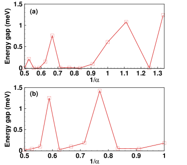
Figure 1: The energy gaps for the filling factor $\nu=-1$ with different $1/\alpha$. (a) The size of the sample is $6a_{0}\times 6a_{0}$. (b) An infinite sample.

In Fig. 1 (a), we show the energy gaps with different $\alpha$. The energy gap oscillates as the magnetic field increases. When $\alpha=1.5$ , which is equivalent to $\alpha=0.5$, a previous study vadym showed that the gap between the two bands would be open when the spin is polarized and one valley is half-filled in the Hartree approximation. In this work, we take the spin into consideration. The ground state is no longer spin polarized. The Zeeman coupling is very weak (about $1$ meV) while the amplitude of the external potential is $20$ meV. The potential is strong enough to mix different spins. The gap for $\alpha=1.5$ is very small in Fig. 1 (a). This is because, intuitively, the two spins are mixed, and the corresponding four bands (two for each spin) in one valley are overlapped to close the Hartree gap. This mixed spin ground state will be discussed in detail in the infinite-size study below.

Figure 2: Energy gaps (a) for $\nu=0$ and (b) for $\nu=4$.

Energy gaps in an infinite sample for $\nu=-1$: The finite-size study however, may not be very reliable. In fact, solution of Eq. (12) is predicated on the size of the sample being infinite. In Fig. 1 (b), the energy gap also oscillates with $1/\alpha$. However, the amplitude and the peaks of the oscillation are changed a little. This might be because the system is size-dependent when the size is finite. For $\alpha=1.5$, the gap is also very small, which is simialr to that of the fintie-size calculation. Generally, the results of the two different calculations are similar. Experimental results (Fig. 4 (c) in yu ) also show oscillations in the energy gap, but the measured gap is nonzero for $\alpha=2$.

Energy gaps in an infinite sample for $\nu=0,4$: We calculate for filling factors $\nu=0,4$, in the LLs $N=0,1$, respectively. In these cases, each LL is half-filled, i.e., there are $N_{s}=2N_{\phi}$ electrons in the LL $0$ or $1$. The spinless picture is obviously not satisfied in this case. We need to consider all the spins and valleys. Figure 2 (a) and Fig. 2 (b) show the energy gaps for the filling factors $\nu=0,4,$ respectively. These two curves are similar: the gaps are very small except at two points $\alpha=1.4,1.6$. Note that for $\alpha=1.5$, the energy gap is small, due to the same reason as what we explained for $\nu=-1$. For the filling factor $\nu=0$, the numerical results are different from the experimental results yu , where the energy gap curve looks like the energy cruve of the charged skyrmion excitation fertig . However, in our calculations we can not obtain such a skyrmion crystal ground state. It might be because the electron density is much higher than what the skyrmion crystal was found numerically cote . The spin or pseudo-spin textures are suppressed by the high density electron gas: (pseudo-) spin flipping can not decrease enough energy to create a (pseudo-) spin texture. The reason why our numerical results differ from the experiment is because perhaps the ground state in the $N=0$ LL is not spin polarized without the external potential young , and we only consider a spin polarized liquid ground state here.

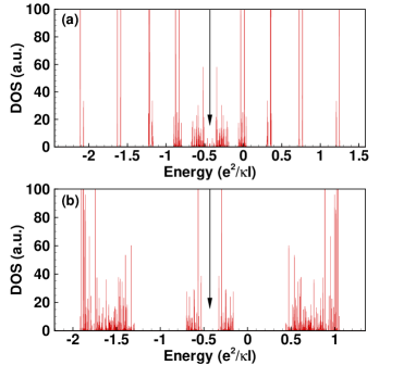
Figure 3: (Color online) The DOS for $\nu=4,$ and (a) for $\alpha=1.1$ and (b) for $\alpha=1.4$. The arrows indicate the Fermi level locations.

For $\nu=4,$ our numerical results are similar to those observed in the experiment yu . In the DOS, we clearly see the energy band structures. The DOS for $\overline{\alpha}\in\left[1.5,2\right]$ is similar to the DOS for $\alpha=3-\overline{\alpha}$, so that we neglect the DOS for $\alpha>1.5$. For simiplicity, we show the DOS curves for $\alpha=1.1$ and $\alpha=1.4$ in Figs. 3 (a) and 3 (b), respectively. For $\alpha=1.1,$ there are ten bands, but the middle two bands touch at the Fermi level. The energy gap is almost zero. Note that some bands far away from the Fermi level split into two sub-bands, due to the Zeeman coupling. For $\alpha=1.4,$ there is a gap between the middle two bands and all bands mix both spins, opening a gap (about 2.5 meV).

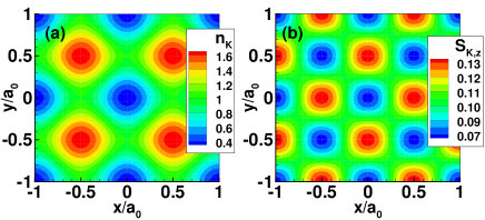
Figure 4: (Color online) (a) Density profile for $\alpha=1.4,\nu=4$, in the $K$ valley. The density is in units of $1/(2\pi\ell^{2})$. (b) The spin field, in units of $\hbar/\left(2\pi\ell^{2}\right),$ in the $z$ direction $S_{K,z}\,\$in the $K$ valley for $\alpha=1.4,\nu=4$ are showed.

We now define the spin field ezawa in valley $\eta$ ($K$ or $K^{\prime}$)

$$S_{\eta,x}+iS_{\eta,y}=\left\langle\rho_{(\eta,\uparrow,(\eta,\downarrow)}\left(\mathbf{r}\right)\right\rangle,$$ (14)

$$S_{\eta,z}=\left\langle\rho_{(\eta,\uparrow),(\eta,\uparrow)}\left(\mathbf{r}\right)-\rho_{(\eta,\downarrow),(\eta,\downarrow)}\left(\mathbf{r}\right)\right\rangle.$$ (15)

The density in valley $k$ is given by $n_{k}\left(\mathbf{r}\right)=\sum_{s}\left\langle\rho_{(\eta,s),(\eta,s)}\left(\mathbf{r}\right)\right\rangle,$ where $s$ is the spin index. The two valleys are completely equivalent in our numerical results, so only the order parameters in the $K$ valley are shown in Fig. 4. The density profiles have the same geometry as the external potential. There is no valley coherence which is not showed in Fig. 4, i.e. $\left\langle\rho_{\left(K,s\right),\left(K^{\prime},s^{\prime}\right)}\right\rangle=0.$ The spin field contains no texture at all, $S_{\eta,x}=S_{\eta,y}=0$, so the electron crystal is not a skyrmion crystal. Only the $z$-components are nonzero, $S_{\eta,z}\neq 0$, and $S_{\eta,z}$ is also crystallized.

Note that the maximum points of $S_{\eta,z}$ do not match the maximum points of the density, where the minimum points of the external potential are. At these points the potential decreases the kinetic energy for both spins. The electrons with both spins overcome the repulsive interaction to be localized by the potential. The density of electrons is minimum at the sites where the energy of the potential is maximum. At the points where the density of electrons is maximum or minimum, the spin field $S_{\eta,z}$ is minimum [the blue dots in Fig. 4 (b)].

In conclusion, we have studied the interacting Hofstadter’s butterfly states in a finite-size system in the HFA in order to study the spin/valley systems such as graphene. We also used a method where the sample is infinite. The energy gaps in the finite-size study agree with the results of the electron crystal qualitatively for filling factor $\nu=-1$. The excitation gap oscillates with the increase of the magnetic field (or $1/\alpha$), similar to a recent experimental observation. For half fillings, we employ the crystal method to calculate the DOS of the system. In the $n=1$ LL, the energy gap in a magnetic field (or $1/\alpha$) agrees well with the experimental results. The osillation of the energy gap agrees qualitatively with that in the experiment, which the nonintearcing picture without spin or valley can not explain. Finally, we show the ground state of the electron gas in the Hofstadter’s butterfly state. The two spins are mixed while there is no valley coherence in the system. This crystal phase is neither like a Wigner crystal nor a skyrmion crystal. The electron gas tends to be in a liquid phase, but the strong external potential crystallizes it. We propose that this method is able to study the interacting (in the HFA) Hofstadter’s butterfly states with different periodic potentials in an infinite system conveniently and efficiently, not only in graphene, but also in other Dirac materials.

The work has been supported by the Canada Research Chairs Program of the Government of Canada.

References

- (1) D. Hofstadter, Phys. Rev. B 14, 2239 (1976); D. Langbein, Phys. Rev. 180, 633 (1969); M.Y. Azbel, Sov. Phys. JETP 19, 634 (1964).
- (2) V. Gudmundsson and R. R. Gerhardts, Phys. Rev. B 52 , 16744 (1995); Surf. Sci. 361-362, 505 (1996); Phys. Rev. B 54, 5223R(1996).
- (3) H. Doh and S. H. Salk, Phys. Rev. B 57, 1312 (1998).
- (4) V. M. Apalkov and T. Chakraborty, Phys. Rev. Lett. 112, 176401 (2014).
- (5) D. Pfannkuche and A. H. MacDonald, Phys. Rev. B 56, R7100 (1997).
- (6) A. Ghazaryan and T. Chakraborty, Phys. Rev. B 91, 125131 (2015).
- (7) D.S.L. Abergel and T. Chakraborty, Phys. Rev. Lett. 102, 056807 (2009); V.M. Apalkov and T. Chakraborty, Phys. Rev. Lett. 97, 126801 (2006); Phys. Rev. Lett. 105, 036801 (2010); Phys. Rev. Lett. 107, 186803 (2011); V.M. Apalkov, T Chakraborty, P Pietiläinen, K Niemelä, Phys. Rev. Lett. 87, 1311 (2001); T. Chakraborty and P. Pietiläinen, Phys. Rev. Lett. 76, 4018 (1996).
- (8) J. Xue, J. Sanchez-Yamagishi, D. Bulmash, P. Jacquod, A. Deshpande, K. Watanabe, T. Taniguchi, P. Jarillo-Herrero and B.J. LeRoy, Nat. Mater. 10, 282-285 (2011).
- (9) R. Decker, Y. Wang, V.W. Brar, W. Regan, H.-Z. Tsai, Q. Wu, W. Gannett, A. Zettl, and M.F. Crommie, Nano Lett. 11, 2291-2295 (2011).
- (10) M. Yankowitz, J. Xue, D. Cormode, J.D. Sanchez-Yamagishi, K. Watanabe, T. Taniguchi, P. Jarillo-Herrero, P. Jacquod, and B.J. LeRoy, Nat. Phys. 8, 382-386 (2012).
- (11) L. A. Ponomarenko, R.V. Gorbachev, G.L. Yu, D.C. Elias, R. Jalil, A.A. Patel, A. Mishchenko, A.S. Mayorov, C.R. Woods, J.R. Wallbank, M. Mucha-Kruczynski, B.A. Piot, M. Potemski, I.V. Grigorieva, K.S. Novoselov, F. Guinea, V.I. Falko, and A.K. Geim, Nature 497, 594-597 (2013).
- (12) C.R. Dean, L. Wang, P. Maher, C. Forsythe, F. Ghahari, Y. Gao, J. Katoch, M. Ishigami, P. Moon, M. Koshino, T. Taniguchi, K. Watanabe, K.L. Shepard, J. Hone, and P. Kim, Nature 497, 598-602 (2013).
- (13) G.L. Yu, R.V. Gorbachev, J.S. Tu, A.V. Kretinin, Y. Cao, R. Jalil, F. Withers, L.A. Ponomarenko, B.A. Piot, M. Potemski, D.C. Elias, X. Chen, K. Watanabe, T. Taniguchi, I.V. Grigorieva, K.S. Novoselov, V.I. Falko, A.K. Geim, and A. Mishchenko, Nat. Phys. 10, 525 (2014).
- (14) N. Nemec and G. Cuniberti, Phys. Rev. B 75, 201404(R) (2007).
- (15) R. Bistritzer and A. H. MacDonald, Phys. Rev. B 84, 035440 (2011).
- (16) P. Moon and M. Koshino, Phys. Rev. B 85, 195458 (2012).
- (17) G. Gumbs, A. Iurov, D. Huang, and L. Zhemchuzhna, Phys. Rev. B 89, 241407(R) (2014).
- (18) M. Diez, J.P. Dahlhaus, M. Wimmer, and C.W.J. Beenakker, Phys. Rev. Lett. 112, 196602 (2014).
- (19) H. Aoki and M.S. Dresselhaus (Eds.), Physics of Graphene (Springer, New York 2014).
- (20) D.S.L. Abergel, V. Apalkov, J. Berashevich, K. Ziegler, T. Chakraborty, Adv. Phys. 59, 261 (2010).
- (21) A.H. Castro Neto, F. Guinea, N.M.R. Peres, K.S. Novoselov, and A.K. Geim, Rev. Mod. Phys. 81,109 (2009).
- (22) M. O. Goerbig, Rev. Mod. Phys. 83,1193 (2011).
- (23) T. Chakraborty and V. M. Apalkov, IET Circuits, Devices & Systems, 9, 19 (2015).
- (24) H.A. Fertig, L. Brey, R. Côté, and A. H. MacDonald, Phys. Rev. B 50, 11018 (1994).
- (25) R. Côté, J.-F. Jobidon, and H. A. Fertig, Phys. Rev. B 78, 085309 (2008).
- (26) R. Côté and A. H. MacDonald, Phys. Rev. Lett. 65, 2662 (1990); Phys. Rev. B 44, 8759 (1991).
- (27) R. Côté, W. Luo, B. Petrov, Yafis Barlas, and A.H. MacDonald, Phys. Rev. B 82, 245307 (2010).
- (28) R. Côté, J.P. Fouquet, and W. Luo, Phys. Rev. B 84, 235301 (2011).
- (29) Y. Barlas, R. Côté and M. Rondeau, Phys. Rev. Lett. 109, 126804 (2012).
- (30) A.F. Young, C.R. Dean, L. Wang, H. Ren, P. Cadden-Zimansky, K. Watanabe, T. Taniguchi, J. Hone, K.L. Shepard, and P. Kim, Nat. Phys. 8, 550–556 (2012).
- (31) Zyun F. Ezawa, Quantum Hall Effects: Field Theoretical Approach and Related Topics, Second Edition. World Scientific, Singapour (2007).