Computational methods for stochastic control with metric interval temporal logic specifications

Abstract

This paper studies an optimal control problem for continuous-time stochastic systems subject to reachability objectives specified in a subclass of metric interval temporal logic specifications, a temporal logic with real-time constraints. We propose a probabilistic method for synthesizing an optimal control policy that maximizes the probability of satisfying a specification based on a discrete approximation of the underlying stochastic system. First, we show that the original problem can be formulated as a stochastic optimal control problem in a state space augmented with finite memory and states of some clock variables. Second, we present a numerical method for computing an optimal policy with which the given specification is satisfied with the maximal probability in point-based semantics in the discrete approximation of the underlying system. We show that the policy obtained in the discrete approximation converges to the optimal one for satisfying the specification in the continuous or dense-time semantics as the discretization becomes finer in both state and time. Finally, we illustrate our approach with a robotic motion planning example.

I Introduction

Stochastic optimal control is an important research area for analysis and control design for continuous-time dynamical systems that operate in the presence of uncertainty. However, existing stochastic control methods cannot be readily applied to handle complex temporal logic specifications with real-time constraints, which are of growing interest to the design of autonomous and semiautonous systems [1, 2, 3, 4]. In this paper, we propose a numerical method for stochastic optimal control with respect to a subclass of metric temporal logic specifications. Particularly, given a specification encoding desirable properties of a continuous-time stochastic system, the task is to synthesize a control policy such that if the system implements the policy, then the probability of a path satisfying the formula is maximized.

Metric temporal logic (MTL) is one of many real-time logics that not only express the relative temporal ordering of events as linear temporal logic (LTL), but also the duration between these events. For example, a surveillance task of a mobile robot, infinitely revisiting region 1 and 2, can be expressed in LTL. But tasks with quantitative timing constraints, for instance, visiting region 2 within 5 minutes after visiting region 1, require the expressive power of MTL. For system specifications in LTL and its untimed variants, methods have been developed for quantitative verification of discrete-time stochastic hybrid systems [5, 6], control design of continuous-time and discrete-time linear stochastic systems [7, 8]. For MTL and its variants, a specification-guided testing framework is proposed in [9] for verification of stochastic cyber-physical systems. Reference [10] proposes a solution to the vehicle routing problem with respect to MTL specifications. Reference [11] develops an abstraction technique and a method of transforming MTL formulas to LTL formulas. As a result, existing synthesis methods for discrete deterministic systems with LTL constraints can be applied to design switching protocols for continuous-time deterministic systems in dynamical environment subject to MTL constraints. Reference [12] proposes a reactive synthesis method to non-deterministic systems with respect to maximizing the robustness of satisfying a specification in signal temporal logic, which is a subclass of MTL. The robustness of a path is measured by the distance between this path and the set of paths that satisfy the specification. Our work differs from existing ones in both the problem formulation and control objective. We deal with systems with stochastic dynamics, rather than non-deterministic systems [12, 11]. We consider reachability objectives specified in metric interval temporal logic (MITL), which is a subclass of MTL. The optimality of control design is evaluated by the probability of satisfying the given specification. The synthesis method is with respect to quantitative criteria (the probability of satisfying the formula), not qualitative criteria (whether the formula is satisfied).

Our solution approach utilizes the Markov chain approximation method [13] to generate a discrete abstraction in the form of a Markov decision process (MDP) approximating the continuous-time stochastic system. Based on a product operation between the discrete abstraction and a finite-state automaton that represents the desirable system property, a near optimal policy with respect to the probability of satisfying the formula in the point-based semantics of MITL [14] can be computed by solving an optimal planning problem in the MDP. We show that as the discretization gets finer in both state space and time space, the optimal control policy in the abstract system converges to the optimal one in the original stochastic system with respect to the probability of satisfying the MITL formula in the continuous or dense-time semantics [15].

II Preliminaries and problem formulation

II-A The system model and timed behaviors

We study stochastic dynamical systems in continuous time. The state of the system evolves according to the stochastic differential equation (SDE)

$$\text{SDE}:\left\{\begin{array}[]{l}dx(t)=f(x(t),u(t))dt+g(x(t))dw,\\ x(0)=x_{0},\end{array}\right.$$ (1)

where $f:X\times U\rightarrow\mathbb{R}^{n}$ and $g:X\rightarrow\mathbb{R}^{n\times k}$ are continuous and bounded functions given $X$ and $U$ as compact state and input space; $w(\cdot)$ is an $\mathbb{R}^{k}$-valued, $\mathcal{F}_{t}$-Wiener process which serves as a “driving noise” and is defined on the probability space $(\Omega,\mathcal{F},P)$; $x(\cdot)$ is an $X$-valued, $\mathcal{F}_{t}$-adapted, measurable process also defined on $(\Omega,\mathcal{F},P)$ and $u(\cdot)$ is an admissible control law, i.e., a $U$-valued, $\mathcal{F}_{t}$-adapted, measurable process defined on $(\Omega,\mathcal{F},P)$. We say $x(\cdot),u(\cdot)$ solve the SDE in (1) provided that

$$x(t)=x(0)+\int_{0}^{t}f(x(\tau),u(\tau))d\tau+\int_{0}^{t}g(x(\tau))dw(\tau),$$ (2)

holds for all time $t\geq 0$.

We introduce a labeling function that relates a sample path of the SDE in (1) to a timed behavior. Let $\mathcal{AP}$ be a finite set of atomic propositions and $L:X\rightarrow 2^{\mathcal{AP}}$ be a labeling function that maps each state $x\in X$ to a set of atomic propositions that evaluate true at that state.

A time interval $I$ is a convex set $\langle t,t^{\prime}\rangle$ where $t,t^{\prime}\in\mathbb{R}_{\geq 0}$, the symbol ‘$\langle$’ can be one of ‘$($’, ‘$[$’, and the symbol ‘$\rangle$’ can be one of ‘$)$’, ‘$]$’, and $t\leq t^{\prime}$. For a time interval of the above form, $t$ and $t^{\prime}$ are left and right end-points, respectively. A time interval is empty if it contains no point. A time interval is singular if $t=t^{\prime}$ and it contains exactly one point.

Definition 1

[16] A dense-time behavior over an infinite-time domain $[0,\infty)$ and a set $\mathcal{AP}$ of atomic propositions is a function $b:[0,\infty)\rightarrow 2^{\mathcal{AP}}$ which maps every time instant $t\geq 0$ to a set $b(t)\in 2^{\mathcal{AP}}$ of atomic propositions that hold at $t$.

Given a continuous sample path $x(\cdot,\omega),\omega\in\Omega$ of the stochastic process $x(\cdot)$, the timed behavior $b$ of this sample path is $b(t)=L(x(t,w))$, for all $t\geq 0$.

Definition 2

[16] Let $b$ be a dense-time behavior and $\delta\in\mathbb{R}_{>0}$ be a positive real number, referred to as the sampling interval. The canonical sampling $b^{\delta}=\{b^{\delta}_{n},n\in\mathbb{Z}_{\geq 0}\}$ of the timed behavior $b$ is defined such that $b^{\delta}_{n}=b(n\delta).$

II-B Specifications

We introduce metric interval temporal logic [15], a subclass of MTL, to express system specifications.

Definition 3 (Metric interval temporal logic)

Given a set $\mathcal{AP}$ of atomic propositions, the formulas of MITL are built from $\mathcal{AP}$ by Boolean connectives and time-constrained versions of the until operator $\cal U$ as follows.

$$\varphi\coloneqq\top\mid\perp\mid\varphi_{1}\land\varphi_{2}\mid\neg\varphi\mid p\mid\varphi_{1}\mathcal{U}_{I}\varphi_{2}$$

where $p\in\mathcal{AP}$, $I$ is a nonsingular time interval with integer end-points, and $\top$, $\perp$ are unconditional true and false, respectively.

Dense-time semantics of MITL

Given a timed behavior $b$, we define $b,t\models\varphi$ with respect to an MITL formula $\varphi$ at time $t$ inductively as follows:

• $b,t\models p$ where $p\in\mathcal{AP}$ if and only if $p\in b(t)$;

• $b,t\models\neg\varphi$ where $b,t\not\models\varphi$;

• $b,t\models\varphi_{1}\land\varphi_{2}$ if and only if $b,t\models\varphi_{1}$ and $b,t\models\varphi_{2}$;

• $b,t\models\varphi_{1}\mathcal{U}_{I}\varphi_{2}$ if and only if there exists $t^{\prime}\in I$ such that $b,t+t^{\prime}\models\varphi_{2}$ and for all $t^{\prime\prime}\in[0,t^{\prime})$, $b,t+t^{\prime\prime}\models\varphi_{1}$;

We write $b\models\varphi$ if $b,0\models\varphi$. We also define temporal operator $\lozenge_{I}\varphi=\top\mathcal{U}_{I}\varphi$ (eventually, $\varphi$ will hold within interval $I$ from now) and $\square_{I}\varphi=\neg(\lozenge_{I}\neg\varphi)$ (for all points within $I$, $\varphi$ holds.)

II-C Timed automata

An MITL formula can be translated into equivalent non-deterministic timed automaton [15]. We consider a fragment of MITL which can be translated into equivalent deterministic timed automaton.

Let $\Sigma$ be a finite alphabet. $\Sigma^{\ast},\Sigma^{\omega}$ are the sets of finite and infinite words (sequences of symbols) over $\Sigma$. A (infinite) timed word [17] over $\Sigma$ is a pair $w=(\tau,\sigma)$, where $\sigma=\sigma_{0}\sigma_{1}\ldots\in\Sigma^{\omega}$ is an infinite word and $\tau=\tau_{0}\tau_{1}\ldots$ is an infinite timed sequence, which satisfies 1) Initialization: $\tau_{0}=0$; 2) Monotonicity: $\tau$ increases strictly monotonically; i.e., $\tau_{i}<\tau_{i+1}$, for all $i\geq 0$; 3) Progress: For every $n\geq 1$ and $\tau_{0}\leq t<\tau_{n}$, there exists some $i\geq 0$, such that $\tau_{i}>t$. The conditions ensure that there are finitely many symbols (events) in a bounded time interval, known as non-Zenoness. We also write $w=(\tau,\sigma)=(\tau_{0},\sigma_{0})(\tau_{1},\sigma_{1})\ldots$.

Before the introduction of timed automata, we introduce clock and clock constraints: Let $C$ be a finite set of clocks, $C=\{c_{1},c_{2},\ldots,c_{M}\}$. We define a set $\Phi_{C}$ of clock constraints over $C$ in the following manner. Let $k\in\mathbb{N}$ be a non-negative integer, and $\bowtie\in\{=,\neq,<,>,\geq,\leq\}$ be a comparison operator,

$$\varphi\coloneqq\top\mid\perp\mid c\bowtie k\mid c-c^{\prime}\bowtie k\mid\varphi_{1}\land\varphi_{2}\mid\varphi_{1}\lor\varphi_{2},$$

where $c,c^{\prime}\in C$ are clocks.

Definition 4

[17] A deterministic timed automaton is a tuple $\mathcal{A}=\langle Q,2^{\mathcal{AP}},\mathsf{Init},F,C,T\rangle$ where $Q$ is a finite set of states, $2^{\mathcal{AP}}$ is a finite set of alphabet with the set $\mathcal{AP}$ of atomic propositions, $\mathsf{Init}$ is the initial state, $F$ is a finite set of accepting states, $C$ is a finite set of clocks. The transition function $T:Q\times 2^{\mathcal{AP}}\times\Phi_{C}\rightarrow Q\times 2^{C}$ is deterministic and interpreted as follows: If $T(q,a,\phi)=(q^{\prime},C^{\prime})$ then $\mathcal{A}$ allows a transition from $q$ to $q^{\prime}$ when the set $a\in 2^{\mathcal{AP}}$ of atomic propositions evaluate true and the clock constraint $\phi\in\Phi_{C}$ is met. After taking this transition, the clocks in $C^{\prime}\subseteq C$ are reset to zero, while other clocks remain unchanged.

For each clock $c_{i}\in C$, we denote $\mathcal{V}_{i}$ the range of that clock. For notational convenience, we define a clock vector $v\in\mathbb{R}^{M}$ where the $i$-th entry $v[i]$ of the clock vector $v$ is the value of clock $c_{i}$, for $i\in\{1,2,\ldots,M\}$. Given $t\in\mathbb{R}_{\geq 0}$, let $v\oplus t=(v[1]+t,v[2]+t,\ldots,v[M]+t)$. We use $\bm{0}$ for the clock vector $v$ where $v[i]=0$ for all $i\in\{1,2,\ldots,M\}$ and $\mathcal{V}=\Pi_{i=1,\ldots,M}\mathcal{V}_{i}$ the set of all possible clock vectors in $\mathcal{A}$. Note that a clock vector is essentially a clock valuation defined in [17].

A configuration of $\mathcal{A}$ is a pair $(q,v)$ where $q$ is a state and $v$ is a clock vector. A transition $T(q,a,\phi)=(q^{\prime},C^{\prime})$ being taken from the configuration $(q,v)$ after $\delta$ time units is also written as $(q,v)\xrightarrow{\delta,a}(q^{\prime},v^{\prime})$ where $v\oplus\delta\models\phi$, and $v^{\prime}[i]=v[i]+\delta$ if $c_{i}\notin C^{\prime}$, otherwise $v^{\prime}[i]=0$.

A run in $\mathcal{A}$ on a timed word $w=(\tau_{0},a_{0})(\tau_{1},a_{1})\ldots$ is an infinite alternating sequence of configurations and delayed transitions $\rho=(\mathsf{Init},\bm{0})\xrightarrow{\Delta\tau_{0},a_{0}}(q_{0},v_{0})\xrightarrow{\Delta\tau_{1},a_{1}}(q_{1},v_{1})\ldots$, with $\Delta\tau_{0}=\tau_{0}$ and $\Delta\tau_{i}=\tau_{i}-\tau_{i-1}$ for $i\geq 1$, subject to the following conditions:

1. There exists $C_{0}\subseteq C$ and $\phi_{0}\in\Phi_{C}$ such that $\bm{0}\oplus\tau_{0}\models\phi_{0}$, $T(\mathsf{Init},a_{0},\phi_{0})=(q_{0},C_{0})$ and $v_{0}[i]=\tau_{0}$ for all $c_{i}\notin C_{0}$ and $v_{0}[i]=0$ for all $c_{i}\in C_{0}$.

2. For each $i\geq 0$, there exist $C_{i+1}\subseteq C$ and $\phi_{i+1}\in\Phi_{C}$ such that $v_{i}\oplus\Delta\tau_{i+1}$ satisfies the clock constraint $\phi_{i+1}$, $T(q_{i},a_{i+1},\phi_{i+1})=(q_{i+1},C_{i+1})$ is defined and $v_{i+1}[k]=v_{i}[k]+\Delta\tau_{i+1}$ for all $c_{k}\notin C_{i+1}$ and $v_{i+1}[k]=0$ for all $c_{k}\in C_{i+1}$.

We consider reachability objectives: A run $\rho$ on a timed word $w$ is accepting if and only if $\mathsf{Occ}(\rho)\cap F\neq\emptyset$ where $\mathsf{Occ}(\rho)$ is the set of states in $Q$ occurring in $\rho$. The set of timed words on which runs are accepted by $\mathcal{A}$ is called the language of $\mathcal{A}$, denoted $\mathcal{L}(\mathcal{A})$.

Example 1

As a simple example of timed automata, let $\mathcal{AP}=\{R_{1}\}$ and the specification formula is $\varphi=\lozenge_{[3,5]}R_{1}$. The reachability specification can be expressed with a deterministic timed automaton $\mathcal{A}_{\varphi}$ in Figure 1. The set of final states is $F=\{q_{1}\}$. The timed automaton accepts a timed word with a prefix $(0,\{\neg R_{1}\})(3.5,\{R_{1}\})$, i.e., $w=(0,\{\neg R_{1}\})(3.5,\{R_{1}\})\ldots$ since $(\mathsf{Init},0)\xrightarrow{0,\{\neg R_{1}\}}(\mathsf{Init},0)\xrightarrow{3.5,\{R_{1}\}}(q_{1},0)$ and $q_{1}$ is accepting. It does not accept $w=(0,\{\neg R_{1}\})(2.8,\{R_{1}\})\ldots$, $w=(\tau,(\{\neg R_{1}\})^{\omega})$ for an arbitrary timed sequence $\tau$, or $w=(0,\{\neg R_{1}\})(6,\{R_{1}\})\ldots$ because either $R_{1}$ is evaluated true when $c<3$ or $c>5$, or it is never true over an infinite timed sequence.

Figure 1: Timed automaton $\mathcal{A}_{\varphi}$ for $\varphi=\lozenge_{[3,5]}R_{1}$. Only one clock $c$ is used. A transition labeled $(a,\phi_{c})$ is taken if and only if both $\phi_{c}$ and $\{a\}$ evaluate true. A transition labeled $(a,\phi_{c},c:=0)$ is taken if and only if both $\phi_{c}$ and $\{a\}$ evaluate true and along with taking the transition, the clock $c$ is reset to $0$.

II-D Problem formulation

Given a sampling interval $\delta$ and a timed behavior $b:[0,\infty)\rightarrow 2^{\mathcal{AP}}$, we map the canonical sampling $b^{\delta}$ of $b$ to a timed word $\mathcal{T}(b^{\delta})=w=(0,\sigma_{0})(\delta,\sigma_{1})\ldots$ such that for any $i\geq 0$, $\sigma_{i}=b(i\delta)$. We say that the timed behavior $b$ satisfies the formula $\varphi$ in the point-based semantics under the sampling interval $\delta$, denoted $b^{\delta}\models\varphi$, if and only if $\mathcal{T}(b^{\delta})$ is accepted in the timed automaton $\mathcal{A}_{\varphi}$ that expresses $\varphi$. The sampling interval $\delta$ determines a sequence of positions (time instances) $0,\delta,2\delta,\ldots$ in the timed behavior. With $\delta$ being a positive infinitesimal, any position in a timed behavior $b$ appears in the timed sequence of the timed word $\mathcal{T}(b^{\delta})$. Thus, we say that the timed behavior $b$ satisfies $\varphi$ in the continuous or dense-time semantics, i.e., $b\models\varphi$, if and only if $\lim_{\delta\rightarrow 0}\mathcal{T}(b^{\delta})\in L(\mathcal{A}_{\varphi})$. A formal definition of satisifiability of MTL formulas over dense-time and point-based semantics is given in [18] and the relation between these two semantics has been studied in [16].

We say that a sample path of the SDE in (1) satisfies an MITL formula $\varphi$ in the dense-time semantics (resp. point-based semantics under the sampling interval $\delta$) if its timed behavior satisfies $\varphi$ in the dense-time semantics (resp. point-based semantics under the sampling interval $\delta$). Formally, let $x(\cdot,w)$ where $w\in\Omega$ be a sample path of the stochastic process $\{x(t),t\geq 0\}$. We have that $\lim_{\delta\rightarrow 0}[L(x(\cdot,w))]^{\delta}\models\varphi$ is equivalent to $L(x(\cdot,w))\models\varphi$.

Given a stochastic process $x(\cdot)$ and an admissible control law $u(\cdot)$ that solve the SDE in (1), the probability of satisfying a formula $\varphi$ in the system under the control law $u(\cdot)$ is the sum of probabilities of continuous sample paths of $x(\cdot)$ that satisfy the formula $\varphi$ in the dense-time or point-based semantics (with respect to a given sampling interval).

Problem 1

Given an SDE in (1) and a timed automaton $\mathcal{A}_{\varphi}=\langle Q,2^{\mathcal{AP}},\mathsf{Init},F,C,T\rangle$ expressing an MITL formula $\varphi$, compute a control input $u(\cdot)$ that maximizes the probability of satisfying $\varphi$ in the dense-time semantics.

III Main result

In this section, we first show that for the SDE in (1), Problem 1 can be formulated as a stochastic optimal control problem in a system derived from the SDE with an augmented state space for capturing relevant properties with respect to its MITL specification. Then, we introduce a numerical scheme that computes an optimal policy in a discrete-approximation of the SDE in (1) with respect to the probability of satisfying the specification in the point-based semantics. The numerical scheme is based on the so-called Markov chain approximation method [13]. We prove that such a policy converges to a solution to Problem 1 as the discretization gets finer.

We make two assumptions.

Assumption 1

The state space $X$ and the clock vector space $\mathcal{V}$ are bounded.

This condition ensures a finite number of states in the discrete approximation. In certain cases, we might also require $U$ to be bounded in order to approximate the input space with a finite set.

Assumption 2

$f(\cdot)$ and $g(\cdot)$ are bounded, continuous, and Lipschitz continuous in state $x$, while $f(\cdot)$ is uniformly so in $u$.

Assumption 2 ensures that the SDE in (1) has a unique solution for a given controller $u(\cdot)$.

III-A Characterizing the reachability probability

For reachability objectives in MITL, Problem 1 is also referred to as the probabilistic reachability problem.

A state in $X\times Q\times\mathcal{V}$ is called a product state, following from the fact that it is a state in a product construction between the stochastic process for the controlled stochastic system and the timed automaton expressing the specification. We define a projection $\pi_{i}$ such that for a given tuple $s$, $\pi_{i}(s)$ is the $i$-th element in the tuple. The projection $\pi_{i}$ is extended to sequences of tuples in the usual way: $\pi_{i}(s\rho)=\pi_{i}(s)\pi_{i}(\rho)$ where $s$ is a tuple and $\rho$ is a sequence of tuples.

Let $S=X\times Q\times\mathcal{V}$. For a stochastic process $\{x(t),t\geq 0\}$, we derive a product stochastic process $\{s(t),t\geq 0\}$ where $s(t)=(x(t),q(t),v(t))$ is a random variable describing the product state. The process $\{s(t),t\geq 0\}$ satisfies the following conditions.

• $s(0)=(x(0),q(0),v(0))$ where $v(0)=\bm{0}$ and $(\mathsf{Init},\bm{0})\xrightarrow{0,L(x(0))}(q(0),\bm{0})$.

• For any time $\tau\in[0,\infty)$, let $\delta=\inf_{t}\big{(}\exists\phi,v(\tau)\oplus t\models\phi\text{ and }T\text{ is defined for }(q(\tau),L(x(\tau+t)),\phi)\big{)}$. If $T(q(\tau),L(x(\tau+\delta)),\phi)=(q^{\prime},C^{\prime})$, then let $q(\tau+\delta)=q^{\prime}$, $v(\tau+\delta)[i]=v(\tau)[i]+\delta$ for $c_{i}\notin C^{\prime}$ and $v(\tau+\delta)[i]=0$ for $c_{i}\in C^{\prime}$. Moreover, for all $\tau\leq t<\tau+\delta$, $q(t)=q(\tau),v(t)=v(\tau)\oplus t$.

Alternatively, given a sample path $x(\cdot,\omega)$, $\omega\in\Omega$, suppose that at time $\tau$ the configuration in $\mathcal{A}_{\varphi}$ is $(q,v)$, the labeling $L(x(\tau+\delta,\omega))$ and the clock vector $v\oplus\delta$ trigger a transition precisely at time $\tau+\delta$ and between the interval $[\tau,\tau+\delta)$, no transition is triggered. Then, the configuration in $\mathcal{A}_{\varphi}$ changes from $(q,v)$ to $(q^{\prime},v^{\prime})$ also at time $\tau+\delta$ provided that $(q,v)\xrightarrow{\delta,L(x(\tau+\delta,\omega))}(q^{\prime},v^{\prime})$. Moreover, for any time $t$ during the time interval $\tau\leq t<\tau+\delta$, the state in the specification automaton remains to be $q$ and each clock increases by $t$ as the time passes.

For a measurable function $f$ that maps sample paths in the process $s(\cdot)$ into reals, we write $E_{s}^{u}(f)$ for the expected value of $f$ when the initial state is $s(0)=s$.

The following lemma is an immediate consequence of the derivation procedure for the product stochastic process.

Lemma 1

Given a set $G=X\times F\times\mathcal{V}$, let $P_{x}(\varphi)$ denote the probability of a sample path in the stochastic process $\{x(t),t\geq 0\}$ starting from $x(0)=x$ and satisfying $\varphi$ in the dense-time semantics and $P_{s}(G)$ is the probability of reaching the set $G$ in the derived product stochastic process $\{s(t),t\geq 0\}$ with $s(0)=s$. It holds that $P_{x}(\varphi)=P_{s}(G).$

By Lemma 1, we can define a value function in the product stochastic process to characterize the probability of satisfying $\varphi$ in the dense-time semantics.

Dense-time reachability probability

The probability of reaching $G$ from a product state $s\notin G$ under a controller $u(\cdot)$ is denoted as $P_{s,u}(G)$. We construct a reward function $r:S\rightarrow\{1,0\}$ such that $r(s)=1_{G}(s)$ where $1_{A}(\cdot)$ is the indicator function, i.e., $1_{A}(x)=1$ if $x\in A$, and $1_{A}(x)=0$ otherwise. Then, $P_{s,u}(G)$ is evaluated by the value function

$$P_{s,u}(G)=W(s,u)=E^{u}_{s}\left\{\int_{0}^{T}r(s(t))dt\right\},$$

where $T$ is a random variable describing the stopping time such that $T=\inf_{t\geq 0}(s(t)\in G)$.

The optimal value function is defined as $V(s)=\sup_{u\in\Pi}W(s,u)$, where $\Pi$ is the set of all admissible control policies for the SDE in (1).

So far, we have shown that given $x(\cdot),u(\cdot)$ that solve the SDE in (1), the probability that a sample path in the stochastic process $x(\cdot)$ satisfies the MITL formula $\varphi$ in the dense-time semantics can be represented by the value $W(s(0),u)$ in the derived product stochastic process $s(\cdot)$ under the reward function $r:S\rightarrow\{1,0\}$.

III-B Markov chain approximation

In this section, we employ the methods in [13] to compute locally consistent Markov chains that approximate the SDE in (1) under a given control policy.

Given an approximating parameter $h$, referred to as the spatial step, we obtain a discretization of the bounded state space, denoted by $X^{h}$, which is a finite set of discrete points approximating $X$. Intuitively, the spatial step $h$ characterizes the distance between neighboring and introduces a partition of $X$. The set of points in the same set of the partition is called an equivalent class. For each $x\in X^{h}$, the set of points in the same equivalent class of $x$ is denoted $[x]=\{x^{\prime}\in X\mid x\leq x^{\prime}<x+h\}$. We call $x\in X^{h}$ the representative point of $[x]$.

We define an MDP $M^{h}=\langle X^{h},U,P^{h},x_{0}\rangle$ where $X^{h}$ is the discrete state space. $U$ is the input space, which can be infinite. $P^{h}:X^{h}\times U\times X^{h}\rightarrow[0,1]$ is the transition probability function (defined later in this section). The initial state is $x_{0}\in X^{h}$ such that the initial state $x(0)$ of the SDE in (1) satisfies $x(0)\in[x_{0}]$.

Definition 5

[13] Let $\Delta t_{i}^{h}$ be the interpolation interval at step $i$ for $i\geq 0$. Let $t_{0}^{h}=0$ and $t_{n}^{h}=\sum_{i=0}^{n-1}\Delta t^{h}_{i}$ for $n\geq 1$ be interpolation times. The continuous interpolations $x^{h}(\cdot),u^{h}(\cdot)$ of the stochastic processes $\{x^{h}_{n},n\in\mathbb{Z}_{\geq 0}\}$ and $\{u_{n}^{h},n\in\mathbb{Z}_{\geq 0}\}$ under the interpolation times $\{t_{n}^{h},n\in\mathbb{Z}_{\geq 0}\}$ are $x^{h}(t)=x_{n}^{h},u^{h}(t)=u_{n}^{h},\text{ for all }t\in[t_{n}^{h},t_{n+1}^{h}).$

Given a policy $\{u_{n},n\in\mathbb{Z}_{\geq 0}\}$, let $\{x_{n},n\in\mathbb{Z}_{\geq 0}\}$ be the induced Markov chain from $M^{h}$ by such a policy. It is shown that if a certain condition is satisfied by the spatial step and the interpolation times, the continuous interpolations of $\{x_{n},n\in\mathbb{Z}_{\geq 0}\}$ and $\{u_{n},n\in\mathbb{Z}_{\geq 0}\}$ converges to processes $x(\cdot)$ and $u(\cdot)$ which solve the SDE in (1).

Theorem 1

[13] Suppose Assumption 2 holds. For any policy $\{u_{n}^{h},n\in\mathbb{Z}_{\geq 0}\}$, let the chain induced from $M^{h}$ by this policy be $\{x^{h}_{n},n\in\mathbb{Z}_{\geq 0}\}$. Let $E_{x,n}^{h,a}$ denote the conditional expectation given $\{x^{h}_{i},u^{h}_{i},0\leq i<n,x^{h}_{n}=x,u^{h}_{n}=a\}$. Then, for all $x\in X$ and $a\in U$, the chain $\{x^{h}_{n},n\in\mathbb{Z}_{\geq 0}\}$ satisfies the local consistency condition:

$$E_{x,n}^{h,a}(\Delta x^{h}_{n})=f(x,a)\Delta t^{h}(x,a)+o(\Delta t^{h}(x,a)),$$

$$E_{x,n}^{h,a}\left(\left[\Delta x^{h}_{n}-E_{x,n}^{h,a}\Delta x^{h}_{n}\right]\left[\Delta x^{h}_{n}-E_{x,n}^{h,a}\Delta x^{h}_{n}\right]^{\prime}\right)$$

$$=g(x)g^{\prime}(x)\Delta t^{h}(x,a)+o(\Delta t^{h}(x,a)),$$

$$\sup_{n,\omega}\lVert\Delta x_{n}^{h}\rVert_{2}\xrightarrow{h}0,$$

where $\Delta x^{h}_{n}=x_{n+1}^{h}-x_{n}^{h}$ is the difference and $\Delta t^{h}(x,a)$ is an appropriate interpolation interval for $x\in X$ and $a\in U$. As $h\rightarrow 0$, the continuous interpolations $x^{h}(\cdot),u^{h}(\cdot)$ of $\{x^{h}_{n},n\in\mathbb{Z}_{\geq 0}\}$ and $\{u_{n}^{h},n\in\mathbb{Z}_{\geq 0}\}$ under the interpolation times $\{t_{n}^{h},n\in\mathbb{Z}_{\geq 0}\}$ computed from the interpolation intervals $\Delta t_{n}^{h}=\Delta t^{h}(x_{n}^{h},u_{n}^{h})$, $n\in\mathbb{Z}_{\geq 0}$, converge in distribution to $x(\cdot),u(\cdot)$ which solve the SDE in (1).

Given a spatial step $h$, under the local consistency condition we construct the MDP $M^{h}$ over the discrete state space $X^{h}$ by computing the transition probability function $P^{h}$ from the parameters of the SDE (see [13] for the details). If the diffusion matrix $g(x)g(x)^{T}$ is diagonal, then the transition probabilities are: $P^{h}(x,a,x\pm h_{i}e_{i})=\Delta t(x,a)\cdot\left[\frac{(g(x)g^{\prime}(x))_{ii}}{2h_{i}^{2}}+\frac{f_{i}^{\pm}(x,a)}{h_{i}}\right],$ and $P^{h}(x,a,x)=1-\Delta t(x,a)\cdot\sum_{i=1}^{n}\left[\frac{(g(x)g^{\prime}(x))_{ii}}{h_{i}^{2}}+\frac{\left|f_{i}(x,a)\right|}{h_{i}}\right],$ where $e_{i}$ is the unit vector in the $i$-th direction and $f_{i}^{\pm}(x,a)=\max(\pm f_{i}(x,a),0)$.

III-C Optimal planning with the discrete approximation

In this section, we construct a product MDP from a discrete approximation of the original system and the timed automaton expressing the system specification. Then, an optimal planning problem is formulated in a product MDP for computing a near-optimal policy for the SDE in (1) with respect to the probability of satisfying the MITL specification in the point-based semantics.

Given the timing constraints in MITL, we consider an explicit approximation method that discretizes both the continuous state space and time. Particularly, instead of computing potentially varying interpolation intervals, we choose a constant interpolation interval $\delta$, referred to as the time step. For the local consistency condition to hold, it is required that for a given $h\in\mathbb{R}^{n}$,

$$\delta\leq\frac{1}{\sum_{i=1}^{n}\left[\frac{(g(x)g^{\prime}(x))_{ii}}{h_{i}^{2}}+\frac{\left|f_{i}(x,a)\right|}{h_{i}}\right]},\forall x\in X,\forall a\in U.$$ (3)

Furthermore, $\delta$ is used as the parameter to discretize the clock vector space $\mathcal{V}$. Let $\mathcal{V}_{i}^{\delta}=\{k\delta\mid 0\leq k\leq\lceil\frac{\max(\mathcal{V}_{i})}{\delta}\rceil\}$ be the discretized space for the range $\mathcal{V}_{i}$ of clock $c_{i}\in C$. The discretized clock vector space is $\mathcal{V}^{\delta}=\Pi_{i=1,\ldots,M}\mathcal{V}_{i}^{\delta}$. Since both $X$ and $\mathcal{V}$ are bounded, sets $X^{h}$ and $\mathcal{V}^{\delta}$ are both finite. The method is “explicit” given the fact that the advance of clock values are explicit: At each step $n$, if the clock is not reset to $0$, then its value is increased by the interpolation interval $\delta$.

Let $d=(h,\delta)$ denote a tuple of spatial and time steps. Next, we construct a product MDP $\mathcal{M}^{d}=M^{h}\times\mathcal{A}_{\varphi}=\langle S^{d},U,P^{d},s_{0}\rangle$ where $S^{d}=X^{h}\times Q\times\mathcal{V}^{\delta}$ is the discrete product state space, $U$ is the input space, $P^{d}:S^{d}\times U\times S^{d}\rightarrow[0,1]$ is the transition probability function, defined as follows. Let $s=(x,q,v)$ and $s^{\prime}=(x^{\prime},q^{\prime},v^{\prime})$. For any $a\in U$, $P^{d}(s,a,s^{\prime})=P^{h}(x,a,x^{\prime})$ if and only if $(q,v)\xrightarrow{\delta,L(x^{\prime})}(q^{\prime},v^{\prime})$. Otherwise $P^{d}(s,a,s^{\prime})=0$. The initial state is $s_{0}=(x_{0},q_{0},\bm{0})$ with $(\mathsf{Init},\bm{0})\xrightarrow{0,L(x_{0})}(q_{0},\bm{0})$.

Assumption 3

There exists a spatial step $h\in\mathbb{R}^{n}$ and a choice of representative points from $X$ such that for all $x\in X^{h}$ and all $x^{\prime}\in[x]$, $L(x^{\prime})=L(x)$.

Lemma 2

Under Assumption 3, given $x(\cdot),u(\cdot)$ that solve the SDE in (1) and a discretization $X^{h}$ of the state space, we construct a discrete chain $\{S_{n},n\in\mathbb{Z}_{\geq 0}\}$ as follows: $S_{0}=s_{0}=(x_{0},q_{0},\bm{0})$ with $x(0)\in[x_{0}]$ and $(\mathsf{Init},\bm{0})\xrightarrow{0,L(x_{0})}(q_{0},\bm{0})$; for all $n\in\mathbb{N}$, $S_{n}=(x^{h}_{n},q_{n},v_{n})$ where $x_{n}^{h}\in X^{h}$ is the representative point to which $x(n\delta)$ belongs, i.e., $x(n\delta)\in[x_{n}^{h}]$, and $(q_{n},v_{n})\xrightarrow{\delta,L(x_{n+1}^{h})}(q_{n+1},v_{n+1})$. The following two statements hold.

1. For all $n\in\mathbb{Z}_{\geq 0}$, the range of the random variable $S_{n}$ is $S^{d}$.

2. The probability of a continuous sample path in $\{x(t),t\geq 0\}$ satisfying $\varphi$ in the point-based semantics under the sampling interval $\delta$ equals the probability of a discrete sample path in the chain $\{S_{n},n\in\mathbb{Z}_{\geq 0}\}$ hitting the set $G^{d}=X^{h}\times F\times\mathcal{V}^{\delta}$. That is,

   $$P_{x(0)}\left([L(x(\cdot))]^{\delta}\models\varphi\right)=\\ P_{s_{0}}(S_{k}\in G^{d}\text{ and }\forall j<k,S_{j}\notin G^{d}).$$

Proof:

To show the first statement, initially, $v(0)=\bm{0}$ is a vector of zeros, which is in $\mathcal{V}^{\delta}$. Suppose that at the $n$-th sampling step $v(n\delta)\in V^{\delta}$, at the next sampling step, for any clock $c_{i}\in C$, either the value of $c_{i}$ is increased by $\delta$ or it is reset to $0$ depending on the current state in the automaton, the clock vector and the current labeling of state in $X$. If the value of $c_{i}$ is reset to $0$, $v((n+1)\delta)[i]=0\in\mathcal{V}_{i}^{\delta}$. Otherwise, $v((n+1)\delta)[i]=v(n\delta)[i]+\delta\in\mathcal{V}_{i}^{\delta}$. By induction, all possible clock vectors we can encounter at the sampling times are in the set $\mathcal{V}^{\delta}$. Thus, the range of a random variable $S_{n}$ for any $n\in\mathbb{Z}_{\geq 0}$ is $S^{d}$, which is a subset of $X^{h}\times Q\times\mathcal{V}$.

Let $x(\cdot,\omega)$ with $\omega\in\Omega$ be a sample path of the process $x(\cdot)$ and $\mathsf{p}=s_{0}s_{1}\ldots$ be the corresponding sample path of the chain $\{S_{n},n\in\mathbb{Z}_{\geq 0}\}$ given the construction method above. Remind that $x(\cdot,\omega)$ satisfies $\varphi$ in the point-based semantics under the sampling interval $\delta$ if and only if the timed word $\mathcal{T}(b^{\delta})$, where $b(\cdot)=L(x(\cdot,w))$, is accepted in $\mathcal{A}_{\varphi}$. Since $x(i\delta,\omega)\in[\pi_{1}(s_{i})]$ for all $i\geq 0$, let $\tau=0\ \delta\ 2\delta\ldots$, we have that the timed word $\mathcal{T}(b^{\delta})=(\tau,L(\pi_{1}(\mathsf{p})))$ by Assumption 3 . Let the run on the timed word $(\tau,L(\pi_{1}(\mathsf{p})))$ be $\rho$ such that $\rho=(\mathsf{Init},\bm{0})\xrightarrow{0,L(\pi_{1}(s_{0}))}(q_{0},v_{0})\xrightarrow{\delta,L(\pi_{1}(s_{1}))}(q_{1},v_{1})\ldots$. By construction, it holds that $q_{i}=\pi_{2}(s_{i})$ and $v_{i}=\pi_{3}(s_{i})$ for all $i\in\mathbb{Z}_{\geq 0}$. By definition of the acceptance condition in $\mathcal{A}_{\varphi}$, $(\tau,L(\pi_{1}(\mathsf{p})))$ is accepted in $\mathcal{A}_{\varphi}$ if and only if $\mathsf{Occ}(\rho)\cap F\neq\emptyset$, which is equivalent to say that for some $k\in\mathbb{Z}_{\geq 0}$, $s_{k}\in X^{h}\times F\times\mathcal{V}$ and for all $j<k$, $s_{j}\notin X^{h}\times F\times\mathcal{V}$. Since in the first statement we have shown that the range of $S_{n}$ for all $n\in\mathbb{Z}_{\geq 0}$ is $S^{d}$, $s_{k}\in X^{h}\times F\times\mathcal{V}^{\delta}=G^{d}$ and the proof for the second statement is complete. ∎

Lemma 2 characterizes the probability of satisfying the specification in point-based semantics under the sampling interval $\delta$ with the probability of reaching a set $G^{d}$ in the product MDP $\mathcal{M}$. Given the objective of maximizing the probability of reaching a set in an MDP, there exists a memoryless and deterministic policy such that by following this policy, from any state, the probability of reaching the set is maximized [19].

We introduce a state $\mathsf{sink}$ into the product MDP $\mathcal{M}^{d}$ and modify $P^{d}$ such that for all $s\in G^{d}$ and all $a\in U$, $P^{d}(s,a,\mathsf{sink})=1$, and for all $a\in U$, $P^{d}(\mathsf{sink},a,\mathsf{sink})=1$, while the other transition probabilities remain unchanged. The product MDP $\mathcal{M}^{d}$ with the augmented state set and the modified transition probability function is denoted $\hat{\mathcal{M}}^{d}$. The reward function $R:S^{d}\cup\{\mathsf{sink}\}\rightarrow\mathbb{R}$ is defined by $R(s)=1_{G^{d}}(s)$. Let $u:S^{d}\cup\{\mathsf{sink}\}\rightarrow U$ be a memoryless and deterministic policy in $\hat{\mathcal{M}}^{d}$ and $\Pi^{d}$ the set of all such policies in $\hat{\mathcal{M}}^{d}$. The value function of policy $u$ is

$$W^{d}(s,u)=E_{s}^{u}\left[\sum_{i=0}^{\infty}R(S_{i})\right],$$

where $\{S_{n},n\in\mathbb{Z}_{\geq 0}\}$ is the Markov chain induced from $\hat{\mathcal{M}}^{d}$ with policy $u$. Thus, the optimal value function $V^{d}(s)=\max_{u\in\Pi^{d}}W^{d}(s,u)$, and the dynamic programming equation is obtained: For $s\in S^{d}$,

$$\begin{split}&V^{d}(s)=R(s)+\max_{a\in U}\left[\sum_{s^{\prime}\in S^{d}\cup\{\mathsf{sink}\}}P^{d}(s,a,s^{\prime})\cdot V^{d}(s^{\prime})\right],\\ &\text{ and }V^{d}(\mathsf{sink})=0.\end{split}$$

Given the optimal policy $\hat{u}^{\ast}:S^{d}\cup\{\mathsf{sink}\}\rightarrow U$ that achieves the maximum value of $V^{d}(s)$ for all $s\in S^{d}$ in the modified product MDP $\hat{\mathcal{M}}^{d}$, we derive a policy $u^{\ast}:S^{d}\rightarrow U$ by letting $u^{\ast}(s)=\hat{u}^{\ast}(s)$. By the definition of reward function and the modified product MDP, policy $u^{\ast}$ maximizes the probability of hitting the set $G^{d}$ in $\mathcal{M}^{d}$.

A policy $u:S^{d}\rightarrow U$ is implemented in the original system in (1) in the following manner. The initial product state is $(x(0),q_{0},\bm{0})$ with $(\mathsf{Init},\bm{0})\xrightarrow{0,L(x(0))}(q_{0},\bm{0})$. At each sampling time $n\delta,n\in\mathbb{Z}_{\geq 0}$, let the current product state be $(x,q,v)\in S$. We compute $(x^{h},q,v)\in S$ such that $x\in[x^{h}]$. Note that at the sampling time the clock vector is always in $\mathcal{V}^{\delta}$ by Lemma 2 and thus $(x^{h},q,v)\in S^{d}$, for which $u$ is defined. Then, we apply a constant input $u((x^{h},q,v))$ during the time interval $[n\delta,(n+1)\delta)$. At the next sampling time $(n+1)\delta$, according to the current state $x^{\prime}$, we compute the state in $\mathcal{A}_{\varphi}$ and the clock vector such that $(q,v)\xrightarrow{\delta,L(x^{\prime})}(q^{\prime},v^{\prime})$. Hence, the new product state is $(x^{\prime},q^{\prime},v^{\prime})$ and a constant control input for the interval $[(n+1)\delta,(n+2)\delta)$ is obtained in the way we just described.

Remark 1

When the input space $U$ for the product MDP is bounded, in the numerical method for the reward maximization problem in the product MDP, in general we also discretize the input space $U$ with some discretization parameter $\epsilon$. Let $U^{\epsilon}$ be the discretized input space. Given the optimal policy $u^{\ast}$ for the product MDP and the optimal policy $u^{\epsilon,\ast}$ in the product MDP with the input space $U^{\epsilon}$, one can derive the bound on $\left|W^{d}(s_{0},u^{\ast})-W^{d}(s_{0},u^{\epsilon,\ast})\right|$ as a function of $\epsilon$, which converges to $0$ as $\epsilon\rightarrow 0$ [20, 13]. Thus, with both discretized state and input space, the implemented policy is near-optimal for the SDE in (1) with respect to the probability of satisfying the MITL specification in the point-based semantics.

III-D Proof of convergence

Based on Theorem 1, we show that the optimal policy synthesized in the product MDP converges to the optimal policy that achieves the maximal probability of satisfying the MITL specification in the dense-time semantics as the discretization in both state space and time space get finer.

Theorem 2

Given a discretization parameter $d=(h,\delta)$ where $\delta$ satisfies the local consistency condition in (3) with respect to the spatial step $h$, it holds that

$$\lim_{h\rightarrow 0}V^{d}(s_{0})=V(s(0)),$$

where $s_{0}=(x_{0},q_{0},\bm{0})$, $s(0)=(x(0),q_{0},\bm{0})$ and $x(0)\in[x_{0}]$.

Proof:

First, it is noted by the local consistency condition and the constraint on $\delta$ in (3), $\delta$ is a decreasing function of $h$ and when $h\rightarrow 0$, $\delta\rightarrow 0$.

For a given $d=(h,\delta)$ where $\delta$ satisfies the constraint in (3) with respect to $h$, let $u^{d}:S^{d}\rightarrow U$ be a policy in the product MDP $\mathcal{M}^{d}$ and $\{S^{d}_{n},n\in\mathbb{Z}_{\geq 0}\}$ be the induced Markov chain. According to Theorem 1, when $h\rightarrow 0$, $\delta\rightarrow 0$ and the continuous interpolations of $\{\pi_{1}(S^{d}_{n}),n\in\mathbb{Z}_{\geq 0}\}$ and $\{u^{d}_{n}=u(S^{d}_{n}),n\in\mathbb{Z}_{\geq 0}\}$ converge in distribution to $x(\cdot)$ and $u(\cdot)$ that solve the SDE in (1). By the determinism in the transition function of the timed automaton and the labeling function, as $h\rightarrow 0$, $\{S^{d}_{n},n\in\mathbb{Z}_{\geq 0}\}$ also converges in distribution to $\{s(t),t\geq 0\}$, which is the product stochastic process derived from $\{x(t),t\geq 0\}$. According to the definition of reward functions $r$ and $R$, since $h\rightarrow 0$, we have $\delta\rightarrow 0$, $x_{0}\rightarrow x(0)$ and $W^{d}(s_{0},\{u^{d}_{n},n\in\mathbb{Z}_{\geq 0}\})$ converges to $W(s(0),\{u(t),t\geq 0\})$.

Now given the optimal control policy $u^{d,\ast}:S^{d}\rightarrow U$ obtained for the product MDP $\mathcal{M}^{d}$, let $\{S_{n},n\in\mathbb{Z}_{\geq 0}\}$ be the Markov chain induced by $u^{d,\ast}$ in $\mathcal{M}^{d}$. We have that $\lim_{h\rightarrow 0}W^{d}(s_{0},\{u^{d,\ast}(S_{n}),n\in\mathbb{Z}_{\geq 0}\})=\lim_{h\rightarrow 0}\sup V^{d}(s_{0})\leq V(s(0))$ by the optimality of the value function $V(s(0))$. On the other hand, let $u^{\ast}=\arg\sup_{u\in\Pi}W(s(0),u)$ be the optimal control policy in the continuous-time stochastic system. We construct a policy $\{u^{\ast}(n\delta),n\in\mathbb{Z}_{\geq 0}\}$ for the product MDP $\mathcal{M}^{d}$ such that the action $u^{\ast}(n\delta)$ is taken at the step $n$. We have $V^{d}(s_{0})\geq W^{d}(s_{0},\{u^{\ast}(n\delta),n\in\mathbb{Z}_{\geq 0}\})$ by the optimality of $V^{d}(s_{0})$. Since $\lim_{h\rightarrow 0}W^{d}(s_{0},\{u^{\ast}(n\delta),n\in\mathbb{Z}_{\geq 0}\})=W(s(0),\{u^{\ast}(t),t\geq 0\})=V(s(0))$, it is inferred that $\lim_{h\rightarrow 0}\inf V^{d}(s_{0})\geq V(s(0))$. Therefore, $\lim_{h\rightarrow 0}V^{d}(s_{0})=V(s(0))$. ∎

IV Example

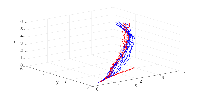
(a) 3D-view

(b) x-y view

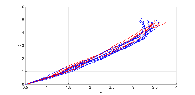
(c) x-t view

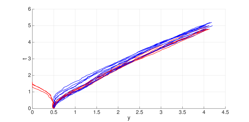
(d) y-t view

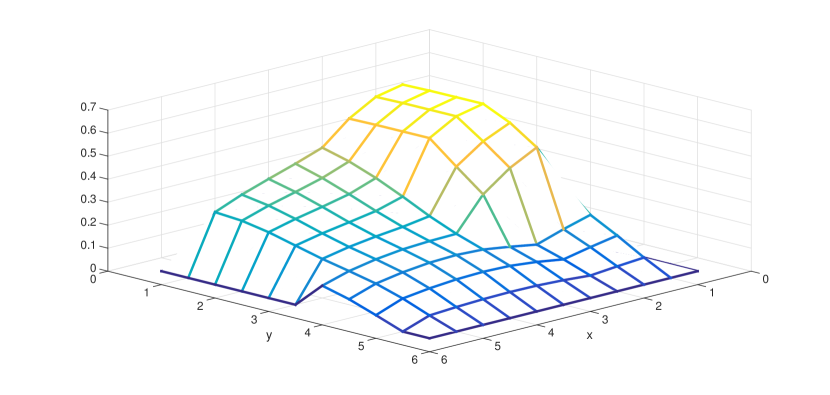
(e) Value function

Figure 2: (a) – (d) Total 20 sample paths for the robot starting at $x_{0}=(0.5,0.5,0)^{T}$ with 3D view, x-y plane view, x-t plane view and y-t plane view. The sample path stops whenever the specification is satisfied, or it does not meet the specification due to time constraints or hitting the walls. Most of the sample paths that fail to satisfy the specification in the point-based semantics reach the region $R_{2}$ prior to the $3$rd time units after visiting $R_{1}$. (e) The value function for the robot with the initial state $\bm{x}_{0}=(x,y,0)^{T}\in X^{h}$, the initial state in the specification timed automaton and the initial clock vector $\bm{0}$.

This section illustrates the method using a motion planning example for a robot modeled as a stochastic Dubin’s car. The dynamics of the system are described by the SDE

$$\underbrace{\begin{bmatrix}dx(t)\\ dy(t)\\ d\theta(t)\end{bmatrix}}_{d\bm{x}(t)}=\underbrace{\begin{bmatrix}v(t)\cos\theta(t)\\ v(t)\sin\theta(t)\\ u(t)\end{bmatrix}dt}_{f(\bm{x}(t),u(t))dt}+g(\bm{x}(t))dw,$$

where $\bm{x}=(x,y,\theta)$ is the coordinate and heading angle of the robot, $v$ is the linear velocity and $u\in U=[-1,1]$ is the angular velocity input. In this example, $v=1$ is fixed and $g(\bm{x}(t))=0.5I_{3}$, and $w(\cdot)$ is a 3-dimensional Wiener process on the probability space $(\Omega,\mathcal{F},P)$.

The workspace of the robot is depicted in Figure 2(b), with two regions $R_{1}$ and $R_{2}$ of importance. The workspace is constrained by the walls $\{(x,y)\mid x\in\{0,5\},0\leq y\leq 5\}\cup\{(x,y)\mid 0\leq x\leq 5,y\in\{0,5\}\}$.

The objective of the robot is to maximize the probability of visiting region $R_{1}$ within the first $5$ time units and after visiting $R_{1}$, reaching $R_{2}$ between the $3$rd and $5$th time units, while avoiding hitting the walls. We define atomic propositions $R_{i}$, $i=1,2$, which evaluates true when the robot is in region $R_{i}$. An atomic proposition $HitWall$ evaluates true if the robot hits the surrounding walls. The MITL formula describing the specification is $\varphi=\lozenge_{[0,5]}((R_{1}\land\neg HitWall)\land\lozenge_{[3,5]}(R_{2}\land\neg HitWall))$. Given an initial state $\bm{x}_{0}$, we want to find an optimal policy that maximizes the probability of $\varphi$ being satisfied. We select a spatial step $h=(0.5,0.5,\pi/4)^{T}$ to obtain a uniform discretization of the state space $X$. Given the choice of $h$, the time step $\delta$ is chosen to be $0.2$ time units for the local consistency condition to hold for all state and control input pairs. The number of states in the MDP $M^{h}$ is $1089$ and the number of product states in the modified product MDP $\hat{\mathcal{M}^{d}}$ is $58809$ (after trimming unreachable states). Remind that the value iteration is polynomial in the size of the MDP $\hat{\mathcal{M}}^{d}$. The implementation are in MATLAB^® on a desktop with Intel(R) Core(TM) processor and 16 GB of memory. The computation of the product MDP takes $18$ minutes and the value iteration converges after $50$ iterations with a pre-specified error tolerance of $0.01$. Each iteration takes about $6$ minutes. In the value iteration we also approximate the input space $U$ with a finite set $U^{\epsilon}$ where $\epsilon=0.2$ is the discretization parameter for the input space.

Since the product state space of the example is $5$-dimensional, we select to plot the optimal value $V^{h}$ for the states with the initial heading angle $\theta=0$, the initial state of the timed automaton and initial clock vector $\bm{0}$ in Figure 2(e). Figures 2(a), 2(b), 2(c), and 2(d) show the sample paths starting from $\bm{x}_{0}=(0.5,0.5,0)$ for a time interval $[0,6]$ from different perspectives. The optimal value $V^{d}(s)$ with $s=((0.5,0.5,0),\mathsf{Init},\bm{0})$ is $0.54$, which is the approximately maximal probability for satisfying $\varphi$ in the point-based semantics under the sampling interval $0.2$ in the system with initial state $\bm{x}(0)=(0.5,0.5,0)$. In simulation, there are $11$ paths (marked in blue) out of $20$ sample paths that satisfy the specification in the point-based semantics.

The drawback of the explicit approach is scalability. In order to compute a control policy with a finer approximation, we need to reduce the spatial step $h$ as well as the time step $\delta$ for the local consistency condition to hold. The product state space becomes very large for a fine discretization. For example, if $h$ is chosen to be $(0.2,0.2,\pi/4)^{T}$, $\delta$ has to be chosen below $0.1$ time units and for the simple example, the product MDP has $608303$ states after trimming. We did not carry out the computation for $V^{h}$ given this finer discretization since it is very time consuming. We discuss the limitation and possible solutions to deal with the issue of scalability in Section V.

V Conclusions and future work

This paper proposes a numerical method based on the Markov chain approximation method for stochastic optimal control with respect to a subclass of quantitive metric temporal logic specifications. We show that as the discretization gets finer, the optimal control policy in the discrete abstract system with respect to satisfying the MITL specification in the point-based semantics converges to the optimal policy in the original system with respect to the dense-time semantics for satisfying the MITL formula. The approach can be easily extended to bounded-time MTL formulas including signal temporal logic formulas. In the future work, we aim to investigate the error bounds introduced by the proposed discrete approximation method. On the other hand, since scalability is a critical issue in the explicit approximation method, we will also investigate a solution approach based on implicit approximation [13]. With implicit approximation method, we can potentially reduce the size of discrete abstract system by treating the clock vector as a state variable, whose discretization parameters are pre-defined and potentially different from the interpolation interval. Parallel algorithms and distributed planning for large-scale MDPs are also considered to handle the issue of scalability.

References

- [1] Z. Manna and A. Pnueli, The Temporal Logic of Reactive and Concurrent Systems: Specifications. Springer Science & Business Media, 1992, vol. 1.
- [2] R. Koymans, “Specifying real-time properties with metric temporal logic,” Real-Time Systems, vol. 2, no. 4, pp. 255–299, 1990.
- [3] G. E. Fainekos, A. Girard, H. Kress-Gazit, and G. J. Pappas, “Temporal logic motion planning for dynamic robots,” Automatica, vol. 45, no. 2, pp. 343–352, 2009.
- [4] T. Wongpiromsarn, U. Topcu, and R. M. Murray, “Receding horizon temporal logic planning,” IEEE Transactions on Automatic Control, vol. 57, no. 11, pp. 2817–2830, 2012.
- [5] A. Abate, J.-P. Katoen, J. Lygeros, and M. Prandini, “Approximate model checking of stochastic hybrid systems,” European Journal of Control, vol. 16, no. 6, pp. 624–641, 2010.
- [6] A. Abate, J.-P. Katoen, and A. Mereacre, “Quantitative automata model checking of autonomous stochastic hybrid systems,” in ACM international conference on Hybrid Systems: Computation and Control, 2011, pp. 83–92.
- [7] M. Lahijanian, S. B. Andersson, and C. Belta, “A probabilistic approach for control of a stochastic system from LTL specifications,” in IEEE Conference on Decision and Control, 2009, pp. 2236–2241.
- [8] M. Svorenova, J. Kretinsky, M. Chmelik, K. Chatterjee, I. Cerna, and C. Belta, “Temporal logic control for stochastic linear systems using abstraction refinement of probabilistic games,” in ACM international conference on Hybrid Systems: Computation and Control, 2015, to appear.
- [9] H. Abbas, B. Hoxha, G. Fainekos, and K. Ueda, “Robustness-guided temporal logic testing and verification for Stochastic Cyber-Physical Systems,” in IEEE Annual International Conference on Cyber Technology in Automation, Control, and Intelligent Systems, 2014, pp. 1–6.
- [10] S. Karaman and E. Frazzoli, “Vehicle routing problem with metric temporal logic specifications,” in IEEE Conference on Decision and Control, 2008, pp. 3953–3958.
- [11] J. Liu and P. Prabhakar, “Switching control of dynamical systems from metric temporal logic specifications,” in IEEE International Conference on Robotics and Automation, 2014, pp. 5333–5338.
- [12] V. Raman, A. Donze, D. Sadigh, R. Murray, and S. A. Seshia, “Reactive synthesis from signal temporal logic specifications,” in ACM international conference on Hybrid Systems: Computation and Control, 2015, to appear.
- [13] H. J. Kushner and P. Dupuis, Numerical Methods for Stochastic Control Problems in Continuous Time. Springer, 2001, vol. 24.
- [14] T. A. Henzinger, “The temporal specification and verification of real-time systems,” Ph.D. dissertation, Citeseer, 1991.
- [15] R. Alur, T. Feder, and T. A. Henzinger, “The benefits of relaxing punctuality,” Journal of the ACM, vol. 43, no. 1, pp. 116–146, Jan. 1996. [Online]. Available: http://doi.acm.org/10.1145/227595.227602
- [16] C. A. Furia and M. Rossi, “A theory of sampling for continuous-time metric temporal logic,” ACM Transactions on Computational Logic, vol. 12, no. 1, p. 8, 2010.
- [17] R. Alur and D. L. Dill, “A theory of timed automata,” Theoretical Computer Science, vol. 126, no. 2, pp. 183 – 235, 1994.
- [18] P. Bouyer, “Model-checking timed temporal logics,” Electronic Notes in Theoretical Computer Science, vol. 231, pp. 323–341, 2009.
- [19] C. Baier and J.-P. Katoen, Principles of Model Checking (Representation and Mind Series). The MIT Press, 2008.
- [20] W. H. Fleming and H. M. Soner, Controlled Markov Processes and Viscosity Solutions. Springer Science & Business Media, 2006, vol. 25.