Semiclassical $S$–matrix for black holes

Abstract

We propose a semiclassical method to calculate ${\cal S}$–matrix elements for two–stage gravitational transitions involving matter collapse into a black hole and evaporation of the latter. The method consistently incorporates back–reaction of the collapsing and emitted quanta on the metric. We illustrate the method in several toy models describing spherical self–gravitating shells in asymptotically flat and AdS space–times. We find that electrically neutral shells reflect via the above collapse–evaporation process with probability $\exp(-B)$, where $B$ is the Bekenstein–Hawking entropy of the intermediate black hole. This is consistent with interpretation of $\exp(B)$ as the number of black hole states. The same expression for the probability is obtained in the case of charged shells if one takes into account instability of the Cauchy horizon of the intermediate Reissner–Nordström black hole. Our semiclassical method opens a new systematic approach to the gravitational ${\cal S}$–matrix in the non–perturbative regime.

1 Introduction

Gravitational scattering has been a subject of intensive research over several decades, see Giddings:2011xs and references therein. Besides being of its own value, this study presents an important step towards resolution of the information paradox — an apparent clash between unitarity of quantum evolution and black hole thermodynamics Hawking:1974sw ; Hawking:1976ra . Recently the interest in this problem has been spurred by the AMPS (or “firewall”) argument Almheiri:2012rt ; Almheiri:2013hfa which suggests that reconciliation of the black hole evaporation with unitarity would require drastic departures from the classical geometry in the vicinity of an old black hole horizon (see Braunstein:2009my1 ; Mathur:2009hf ; Braunstein:2009my for related works). Even the minimal versions of such departures appear to be at odds with the equivalence principle. This calls for putting all steps in the logic leading to this result on a firmer footing.

Unitarity of quantum gravity is strongly supported by the arguments based on AdS/CFT correspondence Maldacena:1997re ; Maldacena:2001kr . This reasoning is, however, indirect and one would like to develop an explicit framework for testing unitarity of black hole evaporation. In particular, one would like to see how the self–consistent quantum evolution leads to the thermal properties of the Hawking radiation and to test the hypothesis Page:1993wv that the information about the initial state producing the black hole is imprinted in subtle correlations between the Hawking quanta.

A natural approach is to view the formation of a black hole and its evaporation as a two–stage scattering transition, see Fig. 1. The initial and final states $\Psi_{i}$ and $\Psi_{f}$ of this process represent free matter particles and free Hawking quanta in flat space–time. They are the asymptotic states of quantum gravity related by an ${\cal S}$–matrix Page:1979tc ; 'tHooft:1996tq ; Giddings:2011xs . Importantly, the black hole itself, being metastable, does not correspond to an asymtotic state. The ${\cal S}$–matrix is unitary if black hole formation does not lead to information loss.

Figure 1: Complete gravitational transition involving formation and evaporation of a black hole.

The importance of collapse stage for addressing the information paradox was emphasized in Alberghi:2001cm ; Vachaspati:2006ki ; Vachaspati:2007hr ; Vachaspati:2007ur ; Brustein:2013qma .

However, calculation of the scattering amplitude for the process in Fig. 1 encounters a formidable obstacle: gravitational interaction becomes strong in the regime of interest and the standard perturbative methods break down Amati:2007ak ; Giddings:2009gj . General considerations Giddings:2009gj supported by the perturbative calculations Amati:2007ak show that scattering of two trans–Planckian particles is accompanied by an increasingly intensive emission of soft quanta as the threshold of black hole formation is approached. While this is consistent with the qualitative properties of the Hawking radiation dominated by many quanta, a detailed comparison is not available. A new perturbative scheme adapted to processes with many particles in the final state has been recently proposed in Dvali:2014ila ; however, its domain of applicability is yet to be understood.

In this paper we follow a different route. We propose to focus on exclusive processes where both initial and final states contain a large number of soft particles. Specifically, one can take $\Psi_{i}$ and $\Psi_{f}$ to be coherent states with large occupation numbers corresponding to the semiclassical wavepackets. We assume that the total energy of the process exceeds the Planck scale, so that the intermediate black hole has mass well above Planckian. Then the overall process is expected to be described within the low–energy gravity. Its amplitude can be evaluated using the semiclassical methods and will yield the black hole ${\cal S}$–matrix in the coherent–state basis Tinyakov:1992dr . A priori, we cannot claim to describe semiclassically the dominant scattering channel with Hawking-like final state which is characterized by low occupation numbers. Still, it seems a safe bet to expect that, within its domain of validity, this approach will provide valuable information on the black hole–mediated amplitudes.

A crucial point in the application of semiclassical methods is the correct choice of the semiclassical solutions. Consider the amplitude

$$\langle\Psi_{f}|\hat{\cal S}|\Psi_{i}\rangle=\int{\cal D}\Phi_{i}{\cal D}\Phi_{f}\;\Psi_{f}^{*}[\Phi_{f}]\;\Psi_{i}[\Phi_{i}]\int{\cal D}\Phi\,\mathrm{e}^{iS[\Phi]/\hbar}$$ (1)

of transition between the initial and final asymptotic states with wave functionals $\Psi_{i}[\Phi_{i}]$ and $\Psi_{f}[\Phi_{f}]$. The path integral in Eq. (1) runs over all fields $\Phi$ of the theory including matter fields, metrics and ghosts from gauge-fixing of the diffeomorphism invariance; $S$ is the action. In the asymptotic past and future the configurations $\Phi$ in Eq. (1) must describe collections of free particles in flat space–time. In the semiclassical approach one evaluates the path integral (1) in the saddle–point approximation. The saddle–point configuration must inherit the correct flat–space asymptotics and, in addition, extremize $S$ i.e. solve the classical equations of motion. However, a naive choice of the solution fails to satisfy the former requirement. Take, for instance, the solution $\Phi_{cl}$ describing the classical collapse. It starts from collapsing particles in flat space–time, but arrives to a black hole in the asymptotic future. It misses the second stage of the scattering process — the black hole decay. Thus, it is not admissible as the saddle point of (1). One faces the task of enforcing the correct asymptotics on the saddle–point configurations.

Furthermore, the saddle–point solutions describing exclusive transitions are generically complex–valued and should be considered in complexified space–time Tinyakov:1992dr ; Rubakov:1992ec . Even subject to appropriate boundary conditions, such solutions are typically not unique. Not all of them are relevant: some describe subdominant processes, some other, when substituted into the semiclassical expression for the amplitude, give nonsensical results implying exponentially large scattering probability. Choosing the dominant physical solution presents a non–trivial challenge.

The method to overcome the two above problems has been developed in Refs. Bezrukov:2003yf ; Bezrukov:2003tg ; Levkov:2007ce ; Levkov:2007yn ; Levkov:2008xx ; Levkov:2009xx in the context of scattering in quantum mechanics with multiple degrees of freedom; it was applied to field theory in Bezrukov:2003er ; Demidov:2011dk . In this paper we adapt this method to the case of gravitational scattering.

It is worth emphasizing the important difference between our approach and perturbative expansion in the classical black hole (or collapsing) geometry, which is often identified with the semiclassical approximation in black hole physics. In the latter case the evaporation is accounted for only at the one–loop level. This approach is likely to suffer from ambiguities associated with the separation of the system into a classical background and quantum fluctuations. Instead, in our method the semiclassical solutions by construction encapsulate black hole decay in the leading order of the semiclassical expansion. They consistently take into account backreaction of the collapsing and emitted matter quanta on the metric. Besides, we will find that the solutions describing the process of Fig. 1 are complex–valued. They bypass, via the complexified evolution, the high–curvature region near the singularity of the intermediate black hole. Thus, one does not encounter the problem of resolving the singularity.

One the other hand, the complex–valued saddle–point configurations do not admit a straightforward interpretation as classical geometries. In particular, they are meaningless for an observer falling into the black hole: the latter measures local correlation functions given by the path integrals in the in–in formalism — with different boundary conditions and different saddle–point configurations as compared to those in Eq. (1). This distinction lies at the heart of the black hole complementarity principle Susskind:1993if .

Our approach can be applied to any gravitational system with no symmetry restrictions. However, the task of solving nonlinear saddle–point equations is rather challenging. In this paper we illustrate the method in several exactly tractable toy models describing spherical gravitating dust shells. We consider neutral and charged shells in asymptotically flat and anti–de Sitter (AdS) space–times. Applications to field theory that are of primary interest are postponed to future.

Although the shell models involve only one collective degree of freedom — the shell radius — they are believed to capture some important features of quantum gravity Berezin:1997fn ; Berezin:1999xa ; Kraus:1994by ; Parikh:1999mf . Indeed, one can crudely regard thin shells as narrow wavepackets of an underlying field theory. In Refs. Berezin:1999nn ; Parikh:1999mf ; Hemming:2000as emission of Hawking quanta by a black hole is modeled as tunneling of spherical shells from under the horizon. The respective emission probability includes back–reaction of the shell on geometry,

$${\cal P}\simeq{\rm e}^{-(B_{i}-B_{f})}\;,$$ (2)

where $B_{i}$ and $B_{f}$ are the Bekenstein–Hawking entropies of the black hole before and after the emission. It has been argued in Parikh:2004ih that this formula is consistent with unitary evolution.

In the context of shell models we consider scattering processes similar to those in Fig. 1: a classical contracting shell forms a black hole and the latter completely decays due to quantum fluctuations into an expanding shell. The initial and final states $\Psi_{i}$ and $\Psi_{f}$ of the process describe free shells in flat or AdS space–times. Our result for the semiclassical amplitude (1) has the form

$$\langle\Psi_{f}|\hat{\cal S}|\Psi_{i}\rangle\simeq\,\mathrm{e}^{iS_{reg}/\hbar}\;.$$ (3)

We stress that it includes backreaction effects. The probability of transition is

$${\cal P}_{fi}\simeq{\rm e}^{-2\mathrm{Im}\,S_{reg}/\hbar}\;.$$

We show that for neutral shells it reproduces Eq. (2) with $B_{i}$ equal to the entropy of the intermediate black hole and $B_{f}=0$. This probability is exponentially small at $M\gg 1$ when the semiclassical approximation is valid. It is consistent with the result of Refs. Berezin:1997fn ; Berezin:1999xa ; Kraus:1994by ; Parikh:1999mf since the first stage of the process, i.e. formation of the intermediate black hole, proceeds classically.

For charged black holes the same result is recovered once we take into account instability of the inner Cauchy horizon of the intermediate Reissner–Nordström black hole Novikov:1980ni ; Poisson:1990eh ; Ori:1991zz ; Brady:1995ni ; Hod:1998gy ; Frolov:2005ps ; Frolov:2006is . Our results are therefore consistent with the interpretation of Hawking radiation as tunneling. However, we obtain important additional information: the phases of the ${\cal S}$–matrix elements which explicitly depend, besides the properties of the intermediate black hole, on the initial and final states of the process.

The paper is organized as follows. In Sec. 2 we introduce general semiclassical method to compute ${\cal S}$–matrix elements for scattering via black hole formation and evaporation. In Sec. 3 we apply the method to transitions of a neutral shell in asymptotically flat space–time. We also discuss relation of the scattering processes to the standard thermal radiation of a black hole. This analysis is generalized in Sec. 4 to a neutral shell in asymptotically AdS space–time where scattering of the shell admits an AdS/CFT interpretation. A model with an electrically charged shell is studied in Sec. 5. Section 6 is devoted to conclusions and discussion of future directions. Appendices contain technical details.

2 Modified semiclassical method

2.1 Semiclassical ${\cal S}$–matrix for gravitational scattering

The ${\cal S}$–matrix is defined as

$$\langle\Psi_{f}|\hat{\cal S}|\Psi_{i}\rangle=\mathrm{lim}_{\tiny\begin{array}[]{l}t_{i}\to-\infty\\ t_{f}\to+\infty\end{array}}\langle\Psi_{f}|\hat{U}_{0}(0,t_{f})\,\hat{U}(t_{f},t_{i})\,\hat{U}_{0}(t_{i},0)|\Psi_{i}\rangle\;,$$ (4)

where $\hat{U}$ is the evolution operator; free evolution operators $\hat{U}_{0}$ on both sides transform from Schrödinger to the interaction picture. In our case $\hat{U}$ describes quantum transition in Fig. 1, while $\hat{U}_{0}$ generates evolution of free matter particles and Hawking quanta in the initial and final states. The time variable $t\in[t_{i},\,t_{f}]$ is chosen to coincide with the time of an asymptotic observer at infinity.

Using the path integrals for the evolution operators and taking their convolutions with the wave functionals of the initial and final states, one obtains the path integral representation for the amplitude (4),

$$\langle\Psi_{f}|\hat{\cal S}|\Psi_{i}\rangle=\int{\cal D}\Phi\,\mathrm{e}^{iS(t_{i},\,t_{f})+iS_{0}(0^{-},\,t_{i})+iS_{0}(t_{f},\,0^{+})}\,\Psi_{i}[\Phi_{-}]\,\Psi_{f}^{*}[\Phi_{+}]\equiv\int{\cal D}\Phi\,{\rm e}^{iS_{tot}[\Phi]}\;,$$ (5)

where $\Phi=\{\phi,\,g_{\mu\nu}\}$ collectively denotes matter and gravitational fields along the time contour in Fig. 2. The quantum measure ${\cal D}\Phi$ should include some ultraviolet regularization as well as gauge–fixing of the diff–invariance and respective ghosts. A non-perturbative definition of this measure presents a well–known challenge. Fortunately, the details of ${\cal D}\Phi$ are irrelevant for our leading–order semiclassical calculations. The interacting and free actions $S$ and $S_{0}$ describe evolution along different parts of the contour. The initial– and final–state wave functionals $\Psi_{i}$ and $\Psi_{f}$ depend on the fields $\Phi_{\mp}\equiv\Phi(t=0^{\mp})$ at the endpoints of the contour. In the second equality of Eq. (5) we combined all factors in the integrand into the “total action” $S_{tot}[\Phi]$. Below we mostly focus on nonlinear evolution from $t_{i}$ to $t_{f}$ and take into account contributions from the dashed parts of the contour in Fig. 2 at the end of the calculation.

Figure 2: The contour used in the calculation of the ${\cal S}$–matrix elements. Quantum transition from $t_{i}$ to $t_{f}$ is preceded and followed by the free evolution.

To distinguish between different scattering regimes, we introduce a parameter $P$ characterizing the initial state Gundlach:2007gc — say, its average energy. If $P$ is small, the gravitational interaction is weak and the particles scatter trivially without forming a black hole. In this regime the integral in Eq. (5) is saturated by the saddle–point configuration $\Phi_{cl}$ satisfying the classical field equations with boundary conditions related to the initial and final states Tinyakov:1992dr . However, if $P$ exceeds a certain critical value $P_{*}$, the classical solution $\Phi_{cl}$ corresponds to formation of a black hole. It therefore fails to interpolate towards the asymptotic out–state $\Psi_{f}$ living in flat space–time. This marks a breakdown of the standard semiclassical method for the amplitude (5).

To deal with this obstacle, we introduce a constraint in the path integral which explicitly guarantees that all field configurations $\Phi$ from the integration domain have flat space–time asymptotics Levkov:2007yn ; Levkov:2008xx ; Levkov:2009xx . Namely, we introduce a functional $T_{int}[\Phi]$ with the following properties: it is (i) diff–invariant; (ii) positive–definite if $\Phi$ is real; (iii) finite if $\Phi$ approaches flat space–time at $t\to\pm\infty$; (iv) divergent for any configuration containing a black hole in the asymptotic future. Roughly speaking, $T_{int}[\Phi]$ measures the “lifetime” of a black hole in the configuration $\Phi$. Possible choices of this functional will be discussed in the next subsection; for now let us assume that it exists. Then we consider the identity

$$1=\int\limits_{0}^{+\infty}dT_{0}\,\delta(T_{int}[\Phi]-T_{0})=\int\limits_{0}^{+\infty}dT_{0}\int\limits_{-i\infty}^{i\infty}\frac{d\epsilon}{2\pi i}\,\mathrm{e}^{\epsilon(T_{0}-T_{int}[\Phi])}\;,$$ (6)

where in the second equality we used the Fourier representation of the $\delta$–function. Inserting Eq. (6) into the integral (5) and changing the order of integration, we obtain,

$$\langle\Psi_{f}|\hat{\cal S}|\Psi_{i}\rangle=\int\frac{dT_{0}d\epsilon}{2\pi i}\;\mathrm{e}^{\epsilon T_{0}}\int{\cal D}\Phi\,\mathrm{e}^{i(S_{tot}[\Phi]+i\epsilon T_{int}[\Phi])}\;.$$ (7)

The inner integral over $\Phi$ in Eq. (7) has the same form as the original path integral, but with the modified action

$$S_{\epsilon}[\Phi]\equiv S_{tot}[\Phi]+i\epsilon T_{int}[\Phi]\;.$$ (8)

By construction, this integral is restricted to configurations $\Phi$ with $T_{int}[\Phi]=T_{0}<\infty$, i.e. the ones approaching flat space–time in the asymptotic past and future. In what follows we make this property explicit by deforming the contour of $\epsilon$–integration to $\mathrm{Re}\,\epsilon>0$. Then configurations with black holes in the final state i.e. with $T_{int}[\Phi]=+\infty$, do not contribute into the integral at all.

By now, we have identically rewritten the integral (5) in the form (7). Its value clearly does not depend on the form of the regulating functional $T_{int}[\Phi]$.

Now the amplitude (7) is computed by evaluating the integrals over $\Phi$, $\epsilon$ and $T_{0}$ one after another in the saddle–point approximation. The saddle–point configuration $\Phi_{\epsilon}$ of the inner integral extremizes the modified action (8), while the saddle–point equation for $\epsilon$ gives the constraint

$$T_{int}[\Phi_{\epsilon}]=T_{0}\;.$$ (9)

This implies that $\Phi_{\epsilon}$ has correct flat–space asymptotics. The integral over $T_{0}$ is saturated at $\epsilon=0$. Importantly, we do not substitute $\epsilon=0$ into the saddle–point equations for $\Phi_{\epsilon}$, since in that case we would recover the original classical equations together with incorrect asymptotics of the saddle–point solutions. Instead, we understand this equation as the limit

$$\epsilon\to+0\;$$ (10)

that must be taken at the last stage of the calculation. The condition $\mathop{\rm Re}\nolimits\epsilon>0$ is required for convergence of the path integral (7). We obtain the saddle–point expression (3) for the amplitude with the exponent

$$S_{reg}=\lim_{\epsilon\to+0}S_{tot}[\Phi_{\epsilon}]\;,$$ (11)

where the limit is taken in the end of the calculation.

Our modified semiclassical method addresses another problem mentioned in the Introduction: it allows to select the relevant saddle–point configurations from the discrete set of complex–valued solutions to the semiclassical equations. As discussed in Bezrukov:2003yf ; Bezrukov:2003tg ; Levkov:2007ce , at $\epsilon>0$ the physical solutions can be obtained from the real classical ones by analytic continuation in the parameters of the in– and out–states. This suggests the following strategy. We pick up a real classical solution $\Phi_{0}$ describing scattering at a small value of the parameter ${P<P_{*}}$. By construction, $\Phi_{0}$ approaches flat space–time at $t\to\mp\infty$ and gives the dominant contribution to the integral (7). Next, we modify the action and gradually increase $\epsilon$ from $\epsilon=0$ to the positive values constructing a continuous branch of modified solutions $\Phi_{\epsilon}$. At $\epsilon\to+0$ these solutions reduce to $\Phi_{0}$ and therefore saturate the integral (7). We increase the value of $P$ to $P>P_{*}$ assuming that continuously deformed saddle–point configurations $\Phi_{\epsilon}$ remain physical. In this way we obtain the modified solutions and the semiclassical amplitude at any $P$. We stress that our continuation procedure cannot be performed with the original classical solutions which, if continued to $P>P_{*}$, describe formation of black holes. On the contrary, the modified solutions $\Phi_{\epsilon}$ interpolate between the flat–space asymptotics at any $P$. They are notably different from the real classical solutions at $P>P_{*}$. At the last step one evaluates the action $S_{tot}$ on the modified solutions and sends $\epsilon\to+0$ obtaining the leading semiclassical exponent of the ${\cal S}$–matrix element, see Eqs. (3), (11).

2.2 The functional $T_{int}[\Phi]$

Let us construct the appropriate functional $T_{int}[\Phi]$. This is particularly simple in the case of reduced models with spherically–symmetric gravitational and matter fields. The general spherically–symmetric metric has the form

$$ds^{2}=\mathrm{g}_{ab}(y)dy^{a}dy^{b}+r^{2}(y)d\Omega^{2}\;,$$ (12)

where $d\Omega$ is the line element on a unit two–sphere and $\mathrm{g}_{ab}$ is the metric in the transverse two–dimensional space. Importantly, the radius $r(y)$ of the sphere transforms as a scalar under the diffeomorphisms of the $y$–manifold. Therefore the functional

$$T_{int}=\int d^{2}y\,\sqrt{-\mathrm{g}}\,w(r)F\big{(}\mathrm{g}^{ab}\partial_{a}r\partial_{b}r\big{)}\;,$$ (13)

is diff–invariant. Here $w(r)$ and $F(\Delta)$ are non–negative functions, so that the functional (13) is positive-definite. We further require that $F(\Delta)$ vanishes if and only if $\Delta=1$. Finally, we assume that $w(r)$ significantly differs from zero only at $r\lesssim r_{w}$, where $r_{w}$ is some fixed value, and falls off sufficiently fast at large $r$. An example of functions satisfying these conditions is $w(r)=\delta(r-r_{w})$, $F(\Delta)=(\Delta-1)^{2}$.

To understand the properties of the functional (13), we consider the Schwarzschild frame where $r$ is the spatial coordinate and the metric is diagonal. The functional (13) takes the form,

$$T_{int}=\int dtdr\sqrt{-\mathrm{g}}\,w(r)F\big{(}\mathrm{g}^{11}\big{)}\;.$$ (14)

Due to fast falloff of $w(r)$ at infinity the integral over $r$ in this expression is finite. However, convergence of the time integral depends on the asymptotics of the metrics in the past and future. In flat space–time $\mathrm{g}^{11}=1$ and the integrand in Eq. (13) vanishes. Thus, the integral over $t$ is finite if $\mathrm{g}_{ab}$ approaches the flat metric at $t\to\pm\infty$. Otherwise the integral diverges. In particular, any classical solution with a black hole in the final state leads to linear divergence at $t\to+\infty$ because the Schwarzschild metric is static and $\mathrm{g}^{11}\neq 1$. Roughly speaking, $T_{int}$ can be regarded as the Schwarzschild time during which matter fields efficiently interact with gravity inside the region $r<r_{w}$. If matter leaves this region in finite time, $T_{int}$ takes finite values. It diverges otherwise. Since the functional (13) is diff–invariant, these properties do not depend on the particular choice of the coordinate system.

The above construction will be sufficient for the purposes of the present paper. Beyond the spherical symmetry one can use the functionals $T_{int}[\Phi]$ that involve, e.g., an integral of the square of the Riemann tensor, or the Arnowitt–Deser–Misner (ADM) mass inside a large volume. Recall the final result for the ${\cal S}$–matrix does not depend on the precise choice of the functional $T_{int}$. Of course, this functional should satisfy the conditions (i)-(iv) listed before Eq. (6).

3 Neutral shell in flat space–time

3.1 The simplest shell model

We illustrate the method of Sec. 2 in the spherically symmetric model of gravity with thin dust shell for matter. The latter is parameterized by a single collective coordinate — the shell radius $r(\tau)$ — depending on the proper time along the shell $\tau$. This is a dramatic simplification as compared to the realistic case of matter described by dynamical fields. Still, one can interprete the shell as a toy model for the evolution of narrow wavepackets in field theory. In particular, one expects that the shell model captures essential features of gravitational transition between such wavepackets.

The minimal action for a spherical dust shell is

$$S_{shell}=-m\int d\tau\;$$ (15)

where $m$ is the shell mass. However, such a shell always collapses into a black hole and hence is not sufficient for our purposes. Indeed, as explained in Sec. 2.1, in order to select the physically relevant semiclassical solutions we need a parameter $P$ such that an initially contracting shell reflects classically at $P<P_{*}$ and forms a black hole at $P>P_{*}$. We therefore generalize the model (15). To this end we assume that the shell is assembled from particles with nonzero angular momenta. At each point on the shell the velocities of the constituent particles are uniformly distributed in the tangential directions, so that the overall configuration is spherically–symmetric. The corresponding shell action is Berezin:2000vv

$$S_{shell}=-\int m_{\mathrm{eff}}\,d\tau\;,\qquad\qquad m_{\mathrm{eff}}^{2}=m^{2}+L^{2}/r^{2}(\tau)\;,$$ (16)

where $L$ is a parameter proportional to the angular momentum of the constituent particles. Its nonzero value provides a centrifugal barrier reflecting classical shells at low energies. Decreasing this parameter, we arrive to the regime of classical gravitational collapse. In what follows we switch between the scattering regimes by changing the parameter $L\equiv P^{-1}$. For completeness we derive the action (16) in Appendix A.

Gravitational sector of the model is described by the Einstein–Hilbert action with the Gibbons–Hawking term,

$$S_{EH}=\frac{1}{16\pi}\int_{\cal V}d^{4}x\sqrt{-g}\,R\;,$$ (17)

$$S_{GH}=\frac{1}{8\pi}\int_{\partial{\cal V}}\kappa\,d^{3}\sigma\,\sqrt{|h|}\,(K-K_{0})\;.$$ (18)

Here the metric $g_{\mu\nu}$ and curvature scalar $R$ are defined inside the space–time volume ${\cal V}$ with the boundary $\partial{\cal V}$. The latter consists of a time–like surface at spatial infinity $r=r_{\infty}\to+\infty$ and space-like surfaces at the initial and final times $t=t_{i,f}\to\mp\infty$. In Eq. (18) $\sigma$ are the coordinates on the boundary, $h$ is the determinant of the induced metric, while $K$ is the extrinsic curvature involving the outer normal. The parameter $\kappa$ equals $+1$ ($-1$) at the time–like (space–like) portions of the boundary. To obtain zero gravitational action in flat space–time, we subtract the regulator $K_{0}$ which is equal to the flat–space extrinsic curvature of the boundary Poisson . For the sphere at infinity $K_{0}=2/r_{\infty}$, while the initial– and final–time hypersurfaces have $K_{0}=0$. The Gibbons–Hawking term (18) will play an important role in our analysis.

Let us first discuss the classical dynamics of the system. Equations of motion follow from variation of the total action

$$S=S_{shell}+S_{EH}+S_{GH}$$ (19)

with respect to the metric $g_{\mu\nu}$ and the shell trajectory $y^{a}(\tau)$. In the regions inside and outside the shell the metric satisfies vacuum Einstein equations and therefore, due to Birkhoff theorem, is given by the flat and Schwarzschild solutions, respectively, see Fig. 3a. Introducing the spherical coordinates $(t_{-},\,r)$ inside the shell and Schwarzschild coordinates $(t_{+},\,r)$ outside, one writes the inner and outer metrics in the universal form

$$ds^{2}_{\pm}=-f_{\pm}(r)dt_{\pm}^{2}+\frac{dr^{2}}{f_{\pm}(r)}+r^{2}d\Omega^{2}\;,$$ (20)

where

$$f_{-}=1\;,\qquad\qquad f_{+}=1-2M/r\;.$$ (21)

The parameter $M$ is the ADM mass which coincides with the total energy of the shell. In what follows we will also use the Schwarzschild radius $r_{h}\equiv 2M$. For the validity of the semiclassical approach we assume that the energy is higher than Planckian, $M\gg 1$.

                 

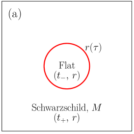
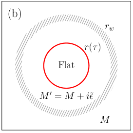
Figure 3: Gravitational field of the spherical dust shell: (a) in the original model, (b) in the model with modification at $r\approx r_{w}$.

Equation for the shell trajectory is derived in Appendix B by matching the inner and outer metrics at the shell worldsheet with the Israel junction conditions Israel:1966rt ; Berezin:1987bc . It can be cast into the form of an equation of motion for a particle with zero energy in an effective potential,

$$\dot{r}^{2}+V_{\mathrm{eff}}(r)=0\;,$$ (22)

$$V_{\mathrm{eff}}=f_{-}-\frac{r^{2}}{4m_{\mathrm{eff}}^{2}}\left(f_{+}-f_{-}-\frac{m_{\mathrm{eff}}^{2}}{r^{2}}\right)^{2}$$ (23)

$$~{}~{}~{}~{}~{}=1-\frac{\left(L^{2}+m^{2}r^{2}+2Mr^{3}\right)^{2}}{4r^{4}(L^{2}+m^{2}r^{2})}\;.$$

This equation incorporates gravitational effects as well as the backreaction of the shell on the spacetime metric. The potential $V_{\mathrm{eff}}(r)$ goes to $-\infty$ at $r\to 0$ and asymptotes to a negative value $1-M^{2}/m^{2}$ at $r=+\infty$, see Fig. 4. At large enough $L$ the potential crosses zero at the points $A$ and $A^{\prime}$ — the turning points of classical motion. A shell coming from infinity reflects from the point $A$ back to $r=+\infty$. When $L$ decreases, the turning points approach each other and coalesce at a certain critical value $L=L_{*}$. At even smaller $L$ the turning points migrate into the complex plane, see Fig. 5 (upper left panel), and the potential barrier disappears. Now a classical shell coming from infinity goes all the way to $r=0$. This is the classical collapse.

Now, we explicitly see an obstacle for finding the reflected semiclassical solutions at $L<L_{*}$ with the method of continuous deformations. Indeed, at large $L$ the reflected solutions $r=r(\tau)$ are implicitly defined as

$$\int\limits^{r(\tau)}\frac{dr}{\sqrt{-V_{\mathrm{eff}}(r)}}=\tau\;,$$ (24)

where the square root is positive at $r\to+\infty+i\,0$. The indefinite integral is performed along the contour ${\cal C}$ running from $r=+\infty-i0$ to $r=+\infty+i0$ and encircling the turning point $A$ — the branch point of the integrand (see the upper left panel of Fig. 5). As $L$ is lowered, the branch point moves and the integration contour stays attached to it. However, at $L=L_{*}$ when the branch points $A$ and $A^{\prime}$ coalesce, the contour ${\cal C}$ is undefined. It is therefore impossible to obtain reflected semiclassical solutions at $L<L_{*}$ from the classical solutions at $L>L_{*}$.

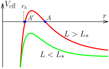
Figure 4: Effective potential for the shell motion.

3.2 Modification

To find physically relevant reflected trajectories at $L<L_{*}$, we use the method of Sec. 2 and add an imaginary term $i\epsilon T_{int}$ to the action. We consider $T_{int}$ of the form (13), where the function $w(r)$ is concentrated in the vicinity of $r=r_{w}$. The radius $r_{w}$ is chosen to be large enough, in particular, larger than the Schwarzschild radius $r_{h}$ and the position $r_{A}$ of the right turning point $A$. Then the Einstein equations are modified only at $r\approx r_{w}$, whereas the geometries inside and outside of this layer are given by the Schwarzschild solutions with masses $M^{\prime}$ and $M$, see Fig. 3b. To connect these masses, we solve the modified Einstein equations in the vicinity of $r_{w}$. Inserting general spherically symmetric metric in the Schwarzschild frame,

$$ds^{2}=-f(t,r)dt^{2}+\frac{dr^{2}}{\tilde{f}(t,r)}+r^{2}d\Omega^{2}\;,$$ (25)

into the $(tt)$ component of Einstein equations, we obtain,

$$\frac{\partial_{r}\tilde{f}}{r}-\frac{1-\tilde{f}}{r^{2}}=\frac{2i\epsilon}{r^{2}}w(r)\,F(\tilde{f})\;.$$ (26)

The solution reads,

$$\tilde{f}=1-\frac{2\tilde{M}(r)}{r}\;,\qquad\mathrm{where}\qquad\tilde{M}(r)=M+i\epsilon\int_{r}^{+\infty}dr^{\prime}w(r^{\prime})F(\tilde{f})\;.$$ (27)

This gives the relation

$$M^{\prime}=M+i\tilde{\epsilon}~{},\qquad\qquad\tilde{\epsilon}=\epsilon\int\limits_{r\approx r_{w}}dr^{\prime}\,wF\;.$$ (28)

Here $\tilde{\epsilon}>0$ is the new parameter of modification. As before, the ADM mass $M$ of the system is conserved in the course of the evolution. It coincides with the initial and final energies of the shell which are, in turn, equal, as will be shown in Sec. 3.3, to the initial– and final–state energies in the quantum scattering problem. Thus, $M$ is real, while the mass $M^{\prime}$ of the Schwarzschild space–time surrounding the shell acquires a positive imaginary part. The shell dynamics in this case is still described by Eq. (22), where $M$ is replaced by $M^{\prime}$ in the potential (23). Below we find semiclassical solutions for small $\tilde{\epsilon}>0$. In the end $\tilde{\epsilon}$ will be sent to zero.

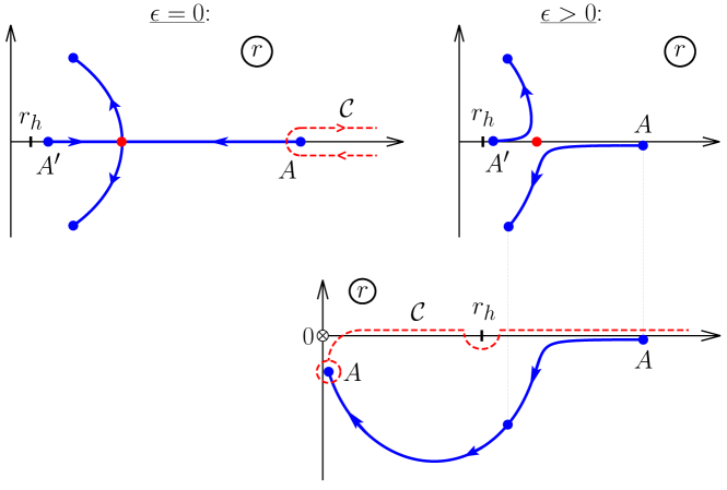
Figure 5: Motion of the turning points in the complex $r$–plane. The points move along the arrows as $L$ decreases. The cases of classical shell (upper left panel) and shell with the modified action (right panels) are shown.

Let us study the effect of the modification (28) on the semiclassical trajectories $r=r(\tau)$ in Eq. (24). At $L>L_{*}$ the complex terms in $V_{\mathrm{eff}}$ are negligible and the reflected trajectory is obtained with the same contour ${\cal C}$ as before, see the upper left panel of Fig. 5. The modification of $V_{\mathrm{eff}}$ becomes important when $L$ gets close to $L_{*}$ and the two turning points $A$ and $A^{\prime}$ approach each other. Expanding the potential in the neighborhood of the maximum, we write,

$$V_{\mathrm{eff}}(r)\approx V_{max}-\mu^{2}(r-r_{max})^{2}\;,$$ (29)

where $V_{max}$, $\mu$ and $r_{max}$ depend on $L$ and $M^{\prime}$. For real $M^{\prime}=M$ the extremal value $V_{max}$ is real and crosses zero when $L$ crosses $L_{*}$, whereas the parameters $\mu^{2}>0$ and $r_{max}$ remain approximately constant. The shift of $M^{\prime}$ into the upper complex half–plane gives a negative imaginary part to $V_{max}$,

$$\mathrm{Im}\,V_{max}=\tilde{\epsilon}\;\frac{\partial V_{max}}{\partial M^{\prime}}+O(\tilde{\epsilon}^{2})<0\;,$$ (30)

where the last inequality follows from the explicit form (23). Now, it is straightforward to track the motion of the turning points using Eq. (29) as $L$ decreases below $L_{*}$. Namely, $A$ and $A^{\prime}$ are shifted into the lower and upper half–planes as shown in Fig. 5 (upper right panel). Importantly, these points never coalesce. Physically relevant reflected solution at $L<L_{*}$ is obtained by continuously deforming the contour of integration in Eq. (24) while keeping it attached to the same turning point. As we anticipated in Sec. 2, a smooth branch of reflected semiclassical solutions parameterized by $L$ exists in the modified system.

If $L$ is slightly smaller than $L_{*}$, the relevant saddle–point trajectories reflect at ${\mathrm{Re}\,r_{A}>r_{h}}$ and hence never cross the horizon. A natural interpretation of the corresponding quantum transitions is over–barrier reflection from the centrifugal potential. However, as $L$ decreases to $L\to 0$, the centrifugal potential vanishes. One expects that the semiclassical trajectories in this limit describe complete gravitational transitions proceeding via formation and decay of a black hole.

After establishing the correspondence between the solutions at $L>L_{*}$ and $L<L_{*}$, we take $\tilde{\epsilon}=0$. This leaves us with the original semiclassical equations which do not include the imaginary regularization terms.

We numerically traced the motion of the turning point $A$ as $L$ decreases from large to small values, see Fig. 5 (lower panel). It approaches the singularity $r=0$ at $L\to 0$. This behavior is confirmed analytically in Appendix C. Thus, at small $L$ the contour ${\cal C}$ goes essentially along the real axis making only a tiny excursion into the complex plane near the singularity. It encircles the horizon $r=r_{h}$ from below.

One remark is in order. For the validity of the low–energy gravity the trajectory should stay in the region of sub-Planckian curvature, $R_{\mu\nu\lambda\rho}R^{\mu\nu\lambda\rho}\sim M^{2}/r^{6}\ll 1$. This translates into the requirement for the turning point

$$|r_{A}|\gg M^{1/3}\;.$$ (31)

On the other hand, we will see shortly that the dependence of the semiclassical amplitude on $L$ drops off at $L\ll L_{*}\sim M^{2}$; we always understand the limit $L\to 0$ in the sense of this inequality. Using the expressions for $r_{A}$ from Appendix C one verifies that the condition (31) can be satisfied simultaneously with $L\ll L_{*}$ in the semiclassical regime $M\gg 1$.

3.3 ${\cal S}$–matrix element

The choice of the time contour.

The action $S_{reg}$ entering the amplitude (3) is computed along the contour in complex plane of the asymptotic observer’s time $t\equiv t_{+}$. Since we have already found the physically relevant contour ${\cal C}$ for $r(\tau)$, let us calculate the Schwarzschild time $t_{+}(r)$ along this contour. We write,

$$t_{+}(r)=\int^{r}dr\;\frac{dt_{+}}{dr}=\int^{r}\frac{dr}{\sqrt{-V_{\rm eff}(r)}}\;\frac{\sqrt{f_{+}(r)-V_{\rm eff}(r)}}{f_{+}(r)}\;,$$ (32)

where the indefinite integral runs along ${\cal C}$. In Eq. (32) we used the the definition of the proper time implying

$$f_{+}\bigg{(}\frac{dt_{+}}{dr}\bigg{)}^{2}=\frac{1}{\dot{r}^{2}}+\frac{1}{f_{+}}\;,$$

and expressed $\dot{r}^{2}$ from Eq. (22). The integrand in Eq. (32) has a pole at the horizon $r=r_{h}$, $f_{+}(r_{h})=0$, which is encircled from below, see Fig. 5, lower panel. The half–residue at this pole contributes $i\pi r_{h}$ to $t_{+}$ each time the contour ${\cal C}$ passes close to it. The contributions have the same sign: although the contour ${\cal C}$ passes the horizon in the opposite directions, the square root in the integrand changes sign after encircling the turning point. Additional imaginary contribution comes from the integral between the real $r$–axis and the turning point $A$; this contribution vanishes at $L\to 0$.

The image ${\cal C}_{t}$ of the contour ${\cal C}$ is shown in Fig. 6, solid line. Adding free evolution from $t_{+}=0^{-}$ to $t_{+}=t_{i}$ and from $t_{+}=t_{f}$ to $t_{+}=0^{+}$ (dashed lines), we obtain the contour analogous to the one in Fig. 2.

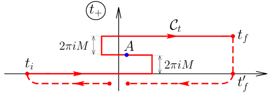
Figure 6: The time contour corresponding to the semiclassical solution at small $L$. Solid and dashed lines correspond to interacting and free evolution respectively, cf. Fig. 2.

One should not worry about the complex value of $t_{f}$ in Fig. 6: the limit $t_{f}\to+\infty$ in the definition of $S$–matrix implies that $S_{reg}$ does not depend on $t_{f}$. Besides, the semiclassical solution $r=r(t_{+})$ is an analytic function of $t_{+}$ and the contour ${\cal C}_{t}$ can be deformed in complex plane as long as it does not cross the singularities of $r(t_{+})$. Below we calculate the action along ${\cal C}_{t}$ because the shell position and the metrics are real in the initial and final parts of this contour. This simplifies the calculation of the Gibbons–Hawking terms at $t_{+}=t_{i}$ and $t_{+}=t_{f}$.

Interacting action.

Now, we evaluate the action of the interacting system $S(t_{i},t_{f})$ entering $S_{reg}$. We rewrite the shell action as

$$S_{shell}=-\int_{\cal C}\frac{dr}{\sqrt{-V_{\rm eff}}}\,m_{\rm eff}\;,$$ (33)

where Eq. (24) was taken into account. The Einstein–Hilbert action (17) is simplified using the trace of the Einstein equations, $R=-8\pi T_{shell\,\mu}^{\phantom{shell}\mu}$, and the energy–momentum tensor of the shell computed in Appendix B, Eq. (98),

$$S_{EH}=\int_{\tau_{i}}^{\tau_{f}}d\tau\,\frac{m^{2}}{2m_{\mathrm{eff}}}=\int_{\cal C}\frac{dr}{\sqrt{-V_{\rm eff}}}\,\frac{m^{2}}{2m_{\mathrm{eff}}}\;.$$ (34)

An important contribution comes from the Gibbons–Hawking term at spatial infinity $r=r_{\infty}\to+\infty$. The extrinsic curvature reads,

$$K\Big{|}_{r_{\infty}}=\frac{rf_{+}^{\prime}+4f_{+}}{2r\sqrt{f_{+}}}\Bigg{|}_{r_{\infty}}=\frac{2}{r_{\infty}}-\frac{M}{r_{\infty}^{2}}+O(r_{\infty}^{-3})\;.$$ (35)

The first term here is canceled by the regulator $K_{0}$ in Eq. (18). The remaining expression is finite at $r_{\infty}\to+\infty$,

$$S_{GH}\Big{|}_{r_{\infty}}=-\frac{M}{2}\int dt_{+}=-\frac{M}{2}\int_{\cal C}\frac{dr}{\sqrt{-V_{\rm eff}}}\,\frac{\sqrt{f_{+}-V_{\rm eff}}}{f_{+}}\;,$$ (36)

where we transformed to integral running along the contour ${\cal C}$ using Eq. (32). Note that this contribution contains an imaginary part

$$\mathop{\rm Im}\nolimits S_{GH}\Big{|}_{r_{\infty}}=-\frac{M}{2}\mathop{\rm Im}\nolimits(t_{f}-t_{i})\;.$$ (37)

Finally, in Appendix D we evaluate the Gibbons–Hawking terms at the initial– and final–time hypersurfaces. The result is

$$S_{GH}\Big{|}_{t_{i,f}}=\frac{\sqrt{M^{2}-m^{2}}}{2}\;r_{i,f}+\frac{M(2M^{2}-m^{2})}{4\sqrt{M^{2}-m^{2}}}\;,$$ (38)

where $r_{i,f}$ are the radii of the shell at the endpoints of the contour ${\cal C}$. The latter radii are real, and so are the terms (38).

Summing up the above contributions, one obtains,

$$S(t_{i},t_{f})=\!\!\int\limits_{\cal C}\!\!\frac{dr}{\sqrt{-V_{\rm eff}}}\bigg{[}\frac{m^{2}-2m^{2}_{\rm eff}}{2m_{\rm eff}}-\frac{M}{2}\frac{\sqrt{f_{+}-V_{\rm eff}}}{f_{+}}\bigg{]}\\ +\frac{\sqrt{M^{2}\!-\!m^{2}}}{2}\,(r_{i}+r_{f})+\frac{M(2M^{2}\!-\!m^{2})}{2\sqrt{M^{2}\!-\!m^{2}}}\,.$$ (39)

This expression contains linear and logarithmic divergences when $r_{i,f}$ are sent to infinity. Note that the divergences appear only in the real part of the action and thus affect only the phase of the reflection amplitude but not its absolute value.

Initial and final–state contributions.

The linear divergence in Eq. (39) is related to free motion of the shell in the asymptotic region ${r\to+\infty}$, whereas the logarithmic one is due to the $1/r$ tails of the gravitational interaction in this region. Though the $1/r$ terms in the Lagrangian represent vanishingly small gravitational forces in the initial and final states, they produce logarithmic divergences in $S(t_{i},t_{f})$ when integrated over the shell trajectory. To obtain a finite matrix element, we include these terms in the definition of the free action $S_{0}$. In Appendix E the latter action is computed for the shell with energy $M$,

$$S_{0}(0^{-},t_{i})=\int_{r_{1}}^{r_{i}}p_{i}(r,M)dr-Mt_{i}\;,~{}~{}~{}~{}~{}~{}~{}S_{0}(t_{f},0^{+})=\int_{r_{f}}^{r_{2}}p_{f}(r,M)dr+Mt_{f}\;,$$ (40)

where $r_{1,2}$ are the positions of the shell at $t_{+}=0^{\mp}$ and

$$p_{i,f}(r,M)=\mp\bigg{[}\sqrt{M^{2}-m^{2}}+\frac{M(2M^{2}-m^{2})}{2r\sqrt{M^{2}-m^{2}}}\bigg{]}$$ (41)

are the initial and final shell momenta with $1/r$ corrections.

The path integral (5) for the amplitude involves free wavefunctions $\Psi_{i}(r_{1})$ and $\Psi_{f}(r_{2})$ of the initial and final states. We consider the semiclassical wavefunctions of the shell with fixed energy $E$,

$$\Psi_{i}(r_{1})\simeq\exp\left\{i\int_{r_{0}}^{r_{1}}p_{i}(r^{\prime},E)dr^{\prime}\right\}\;,\qquad\qquad\Psi_{f}(r_{2})\simeq\exp\left\{i\int_{r_{0}}^{r_{2}}p_{f}(r^{\prime},E)dr^{\prime}\right\}\;,$$ (42)

where $p_{i,f}$ are the same as in Eq. (41). In fact, the energy $E$ is equal to the energy of the semiclassical solution, $E=M$. Indeed, the path integral (5) includes integration over the initial and final configurations of the system, i.e. over $r_{1}$ and $r_{2}$ in the shell model. The condition for the stationary value of $r_{1}$ reads,

$$\frac{\partial}{\partial r_{1}}\log{\Psi_{i}}+i\frac{\partial}{\partial r_{1}}S_{0}(0^{-},t_{i})=0\qquad\Rightarrow\qquad p_{i}(r_{1},E)=p_{i}(r_{1},M)\;,$$ (43)

and similarly for $r_{2}$. This implies equality of $E$ and $M$. Note that the parameter $r_{0}\gg 2M$ in Eq. (42) fixes the phases of the initial and final wavefunctions. Namely, the phases vanish at $r=r_{0}$.

The result.

                

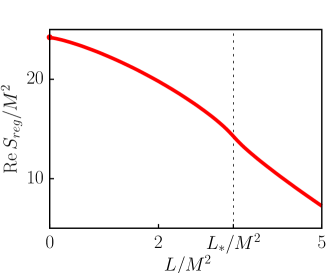
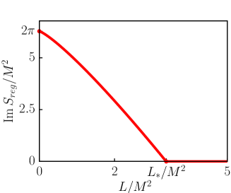
(a)                                                                  (b)

Figure 7: Real (a) and imaginary (b) parts of $S_{reg}$ at $m=0$ as functions of $L$. For the real part we take $r_{0}=10M$.

Combining the contributions (40), (42) with Eq. (39), we obtain the exponent of the ${\cal S}$–matrix element (5),

$$\begin{split}S_{reg}=&\int\limits_{\cal C}\!\!\frac{dr}{\sqrt{-V_{\rm eff}}}\bigg{[}\frac{m^{2}-2m^{2}_{\rm eff}}{2m_{\rm eff}}+\frac{M}{2}\frac{\sqrt{f_{+}-V_{\rm eff}}}{f_{+}}\bigg{]}\\ &-\sqrt{M^{2}-m^{2}}\,\bigg{(}\frac{r_{i}+r_{f}}{2}-2r_{0}\bigg{)}+\frac{M(2M^{2}-m^{2})}{2\sqrt{M^{2}-m^{2}}}\Big{(}1-\log(r_{i}r_{f}/r_{0}^{2})\Big{)}\,.\end{split}$$ (44)

Notice that this result does not depend on any regularization parameters. It is straightforward to check that Eq. (44) is finite in the limit $r_{i,f}\to+\infty$. In Fig. 7 we plot its real and imaginary parts as functions of $L$ for the case of massless shell ($m=0$). The imaginary part vanishes for the values $L\geq L_{*}$ corresponding to classical reflection. At smaller $L$ the imaginary part is positive implying that the reflection probability

$${\cal P}_{fi}\simeq{\rm e}^{-2\mathop{\rm Im}\nolimits S_{reg}}$$

is exponentially suppressed. Importantly, $S_{reg}$ does not receive large contributions from the small–$r$ region near the spacetime singularity. It is therefore not sensitive to the effects of trans–Planckian physics.

In the most interesting case of vanishing centrifugal barrier $L\to 0$ the only imaginary contribution to $S_{reg}$ comes from the residue at the horizon $r_{h}=2M$ in Eq. (44), recall the contour ${\cal C}$ in Fig. 5. The respective value of the suppression exponent is

$$2\mathrm{Im}\,S_{reg}\Big{|}_{L=0}=2\pi M\,\mathrm{Res}_{\,r=r_{h}}\,\frac{\sqrt{f_{+}-V_{\rm eff}}}{\sqrt{-V_{\rm eff}}\;f_{+}}=\pi r_{h}^{2}\;.$$ (45)

This result has important physical implications. First, Eq. (45) depends only on the total energy $M$ of the shell but not on its rest mass $m$. Second, the suppression coincides with the Bekenstein–Hawking entropy of a black hole with mass $M$. The same suppression was obtained in Parikh:1999mf ; Berezin:1999nn for the probability of emitting the total black hole mass in the form of a single shell. We conclude that Eq. (45) admits physical interpretation as the probability of the two–stage reflection process where the black hole is formed in classical collapse with probability of order 1, and decays afterwards into a single shell with exponentially suppressed probability.

One may be puzzled by the fact that, according to Eq. (44), the suppression receives equal contributions from the two parts of the shell trajectory crossing the horizon in the inward and outward directions. Note, however, that the respective parts of the integral (44) do not have individual physical meaning. Indeed, we reduced the original two–dimensional integral for the action to the form (44) by integrating over sections of constant Schwarzschild time. Another choice of the sections would lead to an expression with a different integrand. In particular, using constant–time slices in Painlevé or Finkelstein coordinates one obtains no imaginary contribution to $S_{reg}$ from the inward motion of the shell, whereas the contribution from the outward motion is doubled. The net result for the probability is, of course, the same.

The above result unambiguously shows that the shell model, if taken seriously as a full quantum theory, suffers from the information paradox. Indeed, transition between the only two asymptotic states in this theory — contracting and expanding shell — is exponentially suppressed. Either the theory is intrinsically non–unitary or one has to take into consideration an additional asymptotic state of non–evaporating eternal black hole formed in the scattering process with probability $1-{\cal P}_{fi}$.

On the other hand, the origin of the exponential suppression is clear if one adopts a modest interpretation of the shell model as describing scattering between the narrow wavepackets in field theory. Hawking effect implies that the black hole decays predominantly into configurations with high multiplicity of soft quanta. Its decay into a single hard wavepacket is entropically suppressed. One can therefore argue Parikh:2004ih that the suppression (45) is compatible with unitarity of field theory. However, the analysis of this section is clearly insufficient to make any conclusive statements in the field theoretic context.

As a final remark, let us emphasize that besides the reflection probability our method allows one to calculate the phase of the scattering amplitude $\mathop{\rm Re}\nolimits S_{reg}$. At $L=m=0$ it can be found analytically,

$$\mathop{\rm Re}\nolimits S_{reg}=2Mr_{0}+2M^{2}\log(r_{0}/2M)+M^{2}\;.$$ (46)

Notice that apart from the trivial first term, the phase shift is proportional to the entropy $B\propto M^{2}$; this is compatible with the dependence conjectured in Giddings:2009gj . The phase (46) explicitly depends on the parameter $r_{0}$ of the initial– and final–state wavefunctions.

3.4 Relation to the Hawking radiation

In this section we deviate from the main line of the paper which studies transitions between free–particle initial and final states, and consider scattering of a shell off an eternal pre–existing black hole. This will allow us to establish a closer relation of our approach to the results of Parikh:1999mf ; Berezin:1999nn and the Hawking radiation. We will focus on the scattering probability and thus consider only the imaginary part of the action.

The analysis essentially repeats that of the previous sections with several differences. First of all, the inner and outer space–times of the shell are now Schwarzschild with the metric functions

$$f_{-}=1-2M_{BH}/r\;,\qquad\qquad f_{+}=1-2(M_{BH}+M)/r\;,$$ (47)

where $M_{BH}$ is the eternal black hole mass and $M$ denotes, as before, the energy of the shell. The inner and outer metrics possess horizons at $r_{h}^{-}=2M_{BH}$ and $r_{h}^{+}=2(M_{BH}+M)$, respectively. The shell motion is still described by Eq. (22), where the effective potential is obtained by substituting expressions (47) into the first line of Eq. (23). Next, the global space–time has an additional boundary $r=r_{\infty}^{\prime}\to+\infty$ at the second spatial infinity of the eternal black hole, see Fig. 8. We have to include the corresponding Gibbons–Hawking term, cf. Eq. (36),

$$S_{GH}\Big{|}_{r_{\infty}^{\prime}}=-\frac{M_{BH}}{2}\int dt_{-}\;.$$ (48)

Finally, the eternal black hole in the initial and final states contributes into the free action $S_{0}$. We use the Hamiltonian action of an isolated featureless black hole in empty space–time Kuchar:1994zk ,

$$S_{0,BH}=-M_{BH}\int dt_{+}\;,$$ (49)

where, as usual, the time variable coincides with the asymptotic time. Since we do not equip the black hole with any degrees of freedom, its initial– and final–state wavefunctions are $\Psi_{BH}=1$.

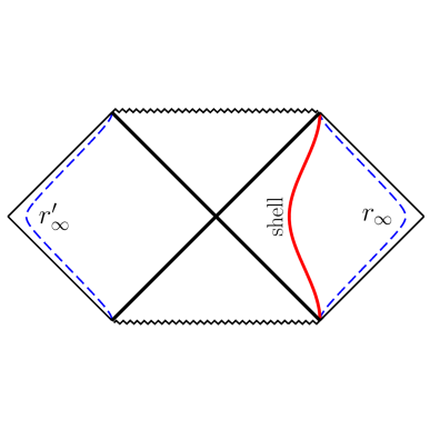
Figure 8: Penrose diagram for scattering of a classical shell from an eternal black hole.

Adding new terms (48), (49) to the action (44), one obtains,

$$\mathrm{Im}\,S_{reg}=\mathrm{Im}\,\int\limits_{\cal C}\frac{dr}{\sqrt{-V_{\rm eff}}}\left[\frac{m^{2}-2m_{\mathrm{eff}}^{2}}{2m_{\mathrm{eff}}}+\frac{M_{BH}+M}{2}\,\frac{\sqrt{f_{+}-V_{\rm eff}}}{f_{+}}\right.\\ \left.-\frac{M_{BH}}{2}\,\frac{\sqrt{f_{-}-V_{\rm eff}}}{f_{-}}\right],$$ (50)

where the integration contour ${\cal C}$ is similar to that in Fig. 5 (lower panel), it bypasses the two horizons $r^{-}_{h}$ and $r_{h}^{+}$ in the lower half of complex $r$–plane. In the interesting limit of vanishing centrifugal barrier $L\to 0$ the imaginary part of the action is again given by the residues at the horizons,

$$2\mathrm{Im}\,S_{reg}\Big{|}_{L=0} =2\pi(M_{BH}+M)\,\mathrm{Res}_{r=r_{h}^{+}}\,\frac{\sqrt{f_{+}-V_{\rm eff}}}{\sqrt{-V_{\rm eff}}\,f_{+}}-2\pi M_{BH}\,\mathrm{Res}_{r=r_{h}^{-}}\,\frac{\sqrt{f_{-}-V_{\rm eff}}}{\sqrt{-V_{\rm eff}}\,f_{-}}$$

$$=\pi\left[(r_{h}^{+})^{2}-(r^{-}_{h})^{2}\right]\;.$$ (51)

Interpretation of this result is similar to that in the previous section. At the first stage of transition the black hole swallows the shell with probability of order one and grows to the mass $M_{BH}+M$. Subsequent emission of the shell with mass $M$ involves suppression

$${\cal P}_{fi}\simeq\mathrm{e}^{-B_{+}+B_{-}}\;,$$ (52)

where $B_{\pm}=\pi(r_{h}^{\pm})^{2}$ are the entropies of the intermediate and final black holes. This suppression coincides with the results of Parikh:1999mf ; Berezin:1999nn .

At $M_{BH}=0$ the process of this section reduces to reflection of a single self-gravitating shell and expression (3.4) coincides with Eq. (45). In the other limiting case ${M\ll M_{BH}}$ the shell moves in external black hole metric without back–reaction. Reflection probability in this case reduces to the Boltzmann exponent

$${\cal P}_{fi}\simeq\mathrm{e}^{-M/T_{H}}\;,$$

where we introduced the Hawking temperature $T_{H}=1/(8\pi M_{BH})$. One concludes that reflection of low–energy shells proceeds via infall into the black hole and Hawking evaporation, whereas at larger $M$ the probability (52) includes back–reaction effects.

3.5 Space–time picture

Let us return to the model with a single shell considered in Secs. 3.1–3.3. In the previous analysis we integrated out the non–dynamical metric degrees of freedom and worked with the semiclassical shell trajectory $(t_{+}(\tau),\,r(\tau))$. It is instructive to visualize this trajectory in regular coordinates of the outer space–time. Below we consider the case of ultrarelativistic shell with small angular momentum: $L\to 0$ and $M\gg m$. One introduces Kruskal coordinates for the outer metric,

$$U=-(r/2M^{\prime}-1)^{1/2}\,\mathrm{e}^{(r-t_{+})/4M^{\prime}}\;,\qquad V=(r/2M^{\prime}-1)^{1/2}\,\mathrm{e}^{(r+t_{+})/4M^{\prime}}\;.$$ (53)

We choose the branch of the square root in these expressions by recalling that $M^{\prime}$ differs from the physical energy $M$ by an infinitesimal imaginary shift, see Eq. (28). The initial part of the shell trajectory from $t_{+}=t_{i}$ to the turning point $A$ (Figs. 5, 6) is approximately mapped to a light ray $V=V_{0}>0$ as shown in Fig. 9. Note that in the limit $L\to 0$ the turning point $A$ is close to the singularity $r=0$, but does not coincide with it. At the turning point the shell reflects and its radius $r(\tau)$ starts increasing with the proper time $\tau$. This means that the shell now moves along the light ray $U=U_{0}>0$, and the direction of $\tau$ is opposite to that of the Kruskal time $U+V$. The corresponding evolution is represented by the interval $(A,t_{f})$ in Fig. 9. We conclude that at $t_{+}=t_{f}$ the shell emerges in the opposite asymptotic region in the Kruskal extension of the black hole geometry. This conclusion may seem puzzling. However, the puzzle is resolved by the observation that the two asymptotic regions are related by analytic continuation in time. Indeed it is clear from Eqs. (53) that the shift $t_{+}\mapsto t_{+}-4\pi Mi$ corresponds to total reflection of Kruskal coordinates $U\to-U$, $V\to-V$. Precisely this time–shift appears if we extend the evolution of the shell to the real time axis (point $t_{f}^{\prime}$ in Fig. 6). At $t_{+}=t_{f}^{\prime}$ the shell emerges in the right asymptotic region with future–directed proper time $\tau$. The process in Fig. 9 can be viewed as a shell–antishell annihilation which is turned by the analytic continuation into the transition of a single shell from $t_{i}$ to $t_{f}^{\prime}$.

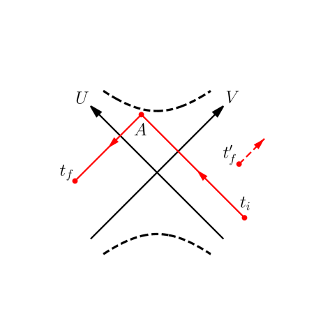
Figure 9: Trajectory of the shell in Kruskal coordinates of the outer metric. Black dashed lines show the singularities $UV=1$.

Now, we write down the space–time metric for the saddle–point solution at $m=0$ and $L\to 0$. Recall that in this case the shell moves along the real $r$–axis. We therefore introduce global complex coordinates $(r,\,t_{+})$, where $t_{+}$ belongs to ${\cal C}_{t}$ and $r$ is real positive. The metric is given by analytic continuation of Eqs. (20), (21),

$$ds^{2}=\begin{cases}-\Big{(}1-\frac{2M^{\prime}}{r_{shell}(t_{+})}\Big{)}^{2}\,dt_{+}^{2}+dr^{2}+r^{2}d\Omega^{2}\;,&r<r_{shell}(t_{+})\\ -\Big{(}1-\frac{2M^{\prime}}{r}\Big{)}\,dt_{+}^{2}+\frac{dr^{2}}{1-\frac{2M^{\prime}}{r}}+r^{2}d\Omega^{2}\;,&r>r_{shell}(t_{+})\;,\end{cases}$$ (54)

where we changed the inner time $t_{-}$ to $t_{+}$ by matching them at the shell worldsheet $r=r_{shell}(t_{+})$. Importantly, the metric (54) is regular at the origin $r=0$ which is never reached by the shell. It is also well defined at $r_{h}=2M$ due to the imaginary part of $M^{\prime}$; in the vicinity of the Schwarzschild horizon $r_{h}$ the metric components are essentially complex. Discontinuity of Eq. (54) at $r=r_{shell}(t_{+})$ is a consequence of the $\delta$–function singularity in the shell energy–momentum tensor. This makes the analytic continuation of the metric ill–defined in the vicinity of the shell trajectory. We expect that this drawback disappears in the realistic field–theory setup where the saddle–point metric will be smooth (and complex–valued) in Schwarzschild coordinates.

4 Massless shell in AdS

4.1 Reflection probability

In this and subsequent sections we subject our method to further tests in more complicated shell models. Here we consider a massless shell in 4-dimensional AdS space-time. The analysis is similar to that of Sec. 3, so we will go fast over details.

The shell action is still given by Eq. (16) with $m_{\rm eff}=L/r$, while the Einstein–Hilbert action is supplemented by the cosmological constant term,

$$S_{EH}=\frac{1}{16\pi}\int_{\cal V}d^{4}x\sqrt{-g}\,(R-2\Lambda)\;.$$ (55)

Here $\Lambda\equiv-3/l^{2}$, $l$ is the AdS radius. The Gibbons–Hawking term has the form (18), where now the regulator at the distant sphere

$$K_{0}\big{|}_{r_{\infty}}=\frac{2}{l}+\frac{l}{r_{\infty}^{2}}$$ (56)

is chosen to cancel the gravitational action of an empty AdS₄. The metric inside and outside the shell is AdS and AdS–Schwarzschild, respectively,

$$f_{-}=1+\frac{r^{2}}{l^{2}}\;,\qquad\qquad f_{+}=1-\frac{2M}{r}+\frac{r^{2}}{l^{2}}\;,$$ (57)

where $M$ is the shell energy. The trajectory of the shell obeys Eq. (22) with the effective potential given by the first line of Eq. (23),

$$V_{\rm eff}=1+\frac{r^{2}}{l^{2}}-\frac{(L^{2}+2Mr^{3})^{2}}{4r^{4}L^{2}}\;.$$ (58)

The $\epsilon$–modification again promotes $M$ in this expression to $M^{\prime}=M+i\tilde{\epsilon}$. Repeating the procedure of Sec. 3.2, we start from the reflected trajectory at large $L$. Keeping $\tilde{\epsilon}>0$, we trace the motion of the turning point as $L$ decreases. The result is a family of contours ${\cal C}$ spanned by the trajectory in the complex $r$–plane. These are similar to the contours in Fig. 5. In particular, at $L\to 0$ the contour ${\cal C}$ mostly runs along the real axis encircling the AdS–Schwarzschild horizon $r_{h}$ from below, as in the lower panel of Fig. 5.

Calculation of the action is somewhat different from that in flat space. First, the space–time curvature is now non-zero everywhere. Trace of the Einstein’s equations gives $R=4\Lambda$. The Einstein–Hilbert action takes the form,

$$S_{EH}=\frac{\Lambda}{2}\bigg{[}\int dt_{-}\int\limits_{0}^{r_{shell}}r^{2}dr+\int dt_{+}\int\limits_{r_{shell}}^{r_{\infty}}r^{2}dr\bigg{]}=\int\limits_{shell}\frac{r^{3}}{2l^{2}}\left(dt_{+}-dt_{-}\right)-\frac{r_{\infty}^{3}}{2l^{2}}\int dt_{+}\;.$$ (59)

The last term diverging at $r_{\infty}\to\infty$ is canceled by the similar contribution in the Gibbons–Hawking term at spatial infinity,

$$S_{GH}\big{|}_{r_{\infty}}=\bigg{(}\frac{r_{\infty}^{3}}{2l^{2}}-\frac{M}{2}\bigg{)}\int dt_{+}\;.$$ (60)

Second, unlike the case of asymptotically flat space–time, Gibbons–Hawking terms at the initial– and final–time hypersurfaces $t_{+}=t_{i,f}$ vanish, see Appendix D. Finally, the canonical momenta of the free shell in AdS,

$$p_{i,f}^{2}(r,M)=\frac{M^{2}}{(1+r^{2}/l^{2})^{2}}-\frac{L^{2}}{r^{2}(1+r^{2}/l^{2})}\;,$$ (61)

are negligible in the asymptotic region $r\to+\infty$. Thus, the terms involving $p_{i,f}$ in the free action (40) and in the initial and final wavefunctions (42) are vanishingly small if the normalization point $r_{0}$ is large enough. This leaves only the temporal contributions in the free actions,

$$S_{0}(0^{-},t_{i})+S_{0}(t_{f},0^{+})=M(t_{f}-t_{i})\;.$$ (62)

Summing up Eqs. (59), (60), (62) and the shell action (16), we obtain,

$$S_{reg} =\int_{\cal C}\frac{dr}{\sqrt{-V_{\rm eff}}}\bigg{[}\frac{r^{3}}{2l^{2}}\bigg{(}\frac{\sqrt{f_{+}-V_{\rm eff}}}{f_{+}}-\frac{\sqrt{f_{-}-V_{\rm eff}}}{f_{-}}\bigg{)}+\frac{M}{2}\frac{\sqrt{f_{+}-V_{\rm eff}}}{f_{+}}-\frac{L}{r}\bigg{]}$$

$$\longrightarrow 2\int_{0}^{\infty}dr\bigg{[}\frac{r^{3}}{2l^{2}}\bigg{(}\frac{1}{f_{+}}-\frac{1}{f_{-}}\bigg{)}+\frac{M}{2f_{+}}\bigg{]}\;\qquad\mbox{at}\qquad L\to 0\;,$$ (63)

where the integration contour in the last expression goes below the pole at $r=r_{h}$. The integral (63) converges at infinity due to fast growth of functions $f_{+}$ and $f_{-}$. In particular, this convergence implies that there are no gravitational self–interactions of the shell in the initial and final states due to screening of infrared effects in AdS.

The imaginary part of Eq. (63) gives the exponent of the reflection probability. It is related to the residue of the integrand at $r_{h}$,

$$2\mathrm{Im}\,S_{reg}=2\pi\bigg{(}\frac{r_{h}^{3}}{l^{2}}+M\bigg{)}\,\mathrm{Res}_{r=r_{h}}\;\frac{1}{f_{+}(r)}=\pi r_{h}^{2}\;.$$ (64)

We again find that the probability is exponentially suppressed by the black hole entropy. Remarkably, the dependence of the reflection probability on the model parameters has combined into $r_{h}$ which is a complicated function of the AdS–Schwarzschild parameters $M$ and $l$.

4.2 AdS/CFT interpretation

Exponential suppression of the shell reflection has a natural interpretation within the AdS/CFT correspondence Maldacena:1997re ; Witten:1998qj ; Gubser:1998bc . The latter establishes relationship between gravity in AdS and strongly interacting conformal field theory (CFT). Consider three–dimensional CFT on a manifold with topology $\mathbb{R}\times S^{2}$ parameterized by time $t$ and spherical angles $\theta$. This is the topology of the AdS₄ boundary, so one can think of the CFT₃ as living on this boundary. Let us build the CFT dual for transitions of a gravitating shell in AdS₄. Assume the CFT₃ has a marginal scalar operator $\hat{O}(t,\theta)$; its conformal dimension is $\Delta=3$. This operator is dual to a massless scalar field $\phi$ in AdS₄.

Consider now the composite operator

$$\hat{O}_{M}(t_{0})=\exp\left\{\int dt\,d^{2}\theta\,G_{M}(t-t_{0})\,\hat{O}(t,\theta)\right\}\;,$$ (65)

where $G_{M}(t)$ is a top–hat function of width $\Delta t\gg 1/M$. This operator is dual to a spherical wavepacket (coherent state) of the $\phi$–field emitted at time $t_{0}$ from the boundary towards the center of AdS Balasubramanian:1998de ; Polchinski:1999ry . With an appropriate normalization of $G_{M}(t)$, the energy of the wavepacket is $M$. Similarly, the operator $\hat{O}_{M}^{+}(t_{0})$ is dual to the wavepacket absorbed on the boundary at time $t_{0}$. Then the correlator

$${\cal G}_{M}=\langle\hat{O}_{M}^{+}(\pi l)\,\hat{O}_{M}(0)\rangle\;$$ (66)

is proportional to the amplitude for reflection of the contracting wavepacket back to the boundary. If the width of the wavepacket is small enough, $\Delta t\ll l$, the $\phi$–field can be treated in the eikonal approximation and the wavepacket follows a sharply defined trajectory. In this way we arrive to the transition of a massless spherical shell in AdS₄, see Fig. 10.

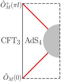
Figure 10: Conformal diagram for scattering of a massless shell in AdS₄. Creation and annihilation of the shell at the AdS boundary correspond to insertions of composite operators in the CFT dual.

Exponential suppression of the transition probability implies respective suppression of the correlator (66). However, the latter suppression is natural in CFT₃ because the state created by the composite operator $\hat{O}_{M}(0)$ is very special. Submitted to time evolution, it evolves into a thermal equilibrium which poorly correlates with the state destroyed by $\hat{O}^{+}_{M}(\pi l)$. Restriction of the full quantum theory in AdS₄ to a single shell is equivalent to a brute–force amputation of states with many soft quanta in unitary CFT₃. Since the latter are mainly produced during thermalization, the amputation procedure leaves us with exponentially suppressed ${\cal S}$–matrix elements.

5 Charged shells

5.1 Elementary shell

Another interesting extension of the shell model is obtained by endowing the shell with electric charge. The corresponding action is the sum of Eq. (19) and the electromagnetic contribution

$$S_{EM}=-\frac{1}{16\pi}\int d^{4}x\sqrt{-g}\,F_{\mu\nu}^{2}-Q\int_{shell}A_{a}dy^{a}\;,$$ (67)

where $A_{\mu}$ is the electromagnetic field with stress tensor $F_{\mu\nu}=\partial_{\mu}A_{\nu}-\partial_{\nu}A_{\mu}$ and $Q$ is the shell charge. This leads to Reissner–Nordström (RN) metric outside the shell and empty flat space–time inside,

$$f_{+}=1-\frac{2M}{r}+\frac{Q^{2}}{r^{2}}\;,\qquad A_{0\,+}=\frac{Q}{r}\;;\qquad\qquad f_{-}=1\;,\qquad A_{0\,-}=0\;.$$ (68)

Other components of $A_{\mu}$ are zero everywhere. Importantly, the outside metric has two horizons

$$r_{h}^{(\pm)}=M\pm\sqrt{M^{2}-Q^{2}}$$ (69)

at $Q<M$. At $Q>M$ the horizons lie in the complex plane, and the shell reflects classically. Since the latter classical reflections proceed without any centrifugal barrier, we set $L=0$ henceforth. The semiclassical trajectories will be obtained by continuous change of the shell charge $Q$.

The evolution of the shell is still described by Eq. (22) with the effective potential constructed from the metric functions (68),

$$V_{\rm eff}=1-\frac{(m^{2}-Q^{2}+2Mr)^{2}}{4m^{2}r^{2}}\;.$$ (70)

This potential always has two turning points on the real axis,

$$r_{A,A^{\prime}}=\frac{Q^{2}-m^{2}}{2(M\mp m)}\;.$$ (71)

The shell reflects classically from the rightmost turning point $r_{A}$ at $Q>M$. In the opposite case $Q<M$ the turning points are covered by the horizons, and the real classical solutions describe black hole formation.

We find the relevant semiclassical solutions at $Q<M$ using $\epsilon$–modification. Since the modification term (13) does not involve the electromagnetic field, it does not affect the charge $Q$ giving, as before, an imaginary shift to the mass, $M\mapsto M+i\tilde{\epsilon}$. A notable difference from the case of Sec. 3 is that the turning points (71) are almost real at $Q<M$. The semiclassical trajectories therefore run close to the real $r$–axis for any $Q$. On the other hand, the horizons (69) approach the real axis with $\mathrm{Im}\,r_{h}^{(+)}>0$ and $\mathrm{Im}\,r_{h}^{(-)}<0$ as $Q$ decreases. Thus, the saddle–point trajectories are defined along the contour ${\cal C}$ in Fig. 11a bypassing $r_{h}^{(+)}$ and $r_{h}^{(-)}$ from below and from above, respectively.

           

(a)                                                                       (b)

Figure 11: Motion of the turning points and the contour ${\cal C}$ defining the trajectory for (a) the model with elementary charged shell and (b) the model with discharge.

Since the semiclassical motion of the shell at $Q<M$ proceeds with almost real $r(\tau)$, we can visualize its trajectory in the extended RN geometry, see Fig. 12. The shell starts in the asymptotic region ${\cal I}$, crosses the outer and inner horizons $r_{h}^{(+)}$ and $r_{h}^{(-)}$, repels from the time–like singularity due to electromagnetic interaction, and finally re–emerges in the asymptotic region ${\cal I}^{\prime}$. At first glance, this trajectory has different topology as compared to the classical reflected solutions at $Q>M$: the latter stay in the region ${\cal I}$ at the final time $t_{+}=t_{f}$. However, following Sec. 3.5 we recall that the Schwarzschild time $t_{+}$ of the semiclassical trajectory is complex in the region ${\cal I}^{\prime}$,

$$\mathrm{Im}\,(t_{f}-t_{i})=\frac{2\pi}{f_{+}^{\prime}(r_{h}^{(+)})}-\frac{2\pi}{f_{+}^{\prime}(r_{h}^{(-)})}\;,$$ (72)

where we used Eq. (32) and denoted by $t_{i}$ and $t_{f}$ the values of $t_{+}$ at the initial and final endpoints of the contour ${\cal C}$ in Fig.11a. Continuing $t_{f}$ to real values, we obtain the semiclassical trajectory arriving to the region ${\cal I}$ in the infinite future, cf. Sec. 3.5. This is what one expects since the asymptotic behavior of the semiclassical trajectories is not changed in the course of continuous deformations.

Figure 12: Conformal diagram for the extended Reissner–Nordström space–time. Semiclassical trajectory running along the contour ${\cal C}$ in Fig. 11a is shown by the red line. The grey region does not exist in theories with dynamical charged fields.

Let us now evaluate the reflection probability. Although the contour ${\cal C}$ is real, it receives imaginary contributions from the residues at the horizons. Imaginary part of the total action comes from Eq. (44) and the electromagnetic term (67). The latter takes the form,

$$S_{EM}=-\int d^{4}x\sqrt{-g}\bigg{(}\frac{F_{\mu\nu}^{2}}{16\pi}+A_{\mu}j^{\mu}\bigg{)}=\frac{1}{16\pi}\int d^{4}x\sqrt{-g}\,F_{\mu\nu}^{2}\;,$$ (73)

where we introduced the shell current $j^{\mu}$, used Maxwell equations $\nabla_{\mu}F^{\mu\nu}=4\pi j^{\nu}$ and integrated by parts. From Eq. (68) we find,

$$S_{EM}=\frac{1}{4}\int dt_{+}\int\limits_{r_{shell}}^{\infty}r^{2}dr\bigg{(}-\frac{2Q^{2}}{r^{4}}\bigg{)}=-\frac{Q^{2}}{2}\int\limits_{shell}\frac{dt_{+}}{r}\;.$$ (74)

Combining this with Eq. (44), we obtain,

$$2\mathrm{Im}\,S_{reg}= \mathrm{Im}\,\int_{\cal C}\frac{dr}{\sqrt{-V_{\rm eff}}}\bigg{[}-m+\bigg{(}M-\frac{Q^{2}}{r}\bigg{)}\frac{\sqrt{f_{+}-V_{\rm eff}}}{f_{+}}\bigg{]}$$

$$= 2\pi\big{[}\mathrm{Res}_{r=r_{h}^{(+)}}-\mathrm{Res}_{r=r_{h}^{(-)}}\big{]}\bigg{(}M-\frac{Q^{2}}{r}\bigg{)}\frac{1}{f_{+}(r)}=\pi\big{(}r_{h}^{(+)}\big{)}^{2}-\pi\big{(}r_{h}^{(-)}\big{)}^{2}\;.$$ (75)

After non–trivial cancellation we again arrive to a rather simple expression. However, this time $2\mathrm{Im}\,S_{tot}$ is not equal to the entropy of the RN black hole, $B_{RN}=\pi\big{(}r_{h}^{(+)}\big{)}^{2}$.

The physical interpretation of this result is unclear. We believe that it is an artifact of viewing the charged shell as an elementary object. Indeed, in quantum mechanics of an elementary shell the reflection probability should vanish at the brink $Q=M$ of classically allowed transitions. It cannot be equal to $B_{RN}$ which does not have this property unlike the expression (75). We now explain how the result is altered in a more realistic setup.

5.2 Model with discharge

Recall that the inner structure of charged black holes in theories with dynamical fields is different from the maximal extension of the RN metric. Namely, the RN Cauchy horizon $r_{h}^{(-)}$ suffers from instability due to mass inflation and turns into a singularity Poisson:1990eh ; Ori:1991zz ; Brady:1995ni ; Hod:1998gy . Besides, pair creation of charged particles forces the singularity to discharge Novikov:1980ni ; Frolov:2005ps ; Frolov:2006is . As a result, the geometry near the singularity resembles that of a Schwarzschild black hole, and the singularity itself is space-like. The part of the maximally extended RN space–time including the Cauchy horizon and beyond (the grey region in Fig. 12) is never formed in classical collapse.

Let us mimic the above discharge phenomenon in the model of a single shell. Although gauge invariance forbids non–conservation of the shell charge $Q$, we can achieve essentially the same effect on the space–time geometry by switching off the electromagnetic interaction at $r\to 0$. To this end we assume spherical symmetry and introduce a dependence of the electromagnetic coupling on the radius. This leads to the action

$$S_{EM}^{\prime}=-\frac{1}{16\pi}\int d^{4}x\sqrt{-g}\,\frac{F_{\mu\nu}^{2}}{e^{2}(r/Q)}\,-Q\int\limits_{shell}A_{a}dy^{a}\;,$$ (76)

where $e(x)$ is a positive form–factor starting from $e=0$ at $x=0$ and approaching $e\to 1$ at $x\to+\infty$. We further assume

$$e(x)<x\;,$$ (77)

the meaning of this assumption will become clear shortly. Note that the action (76) is invariant under gauge transformations, as well as diffeomorphisms preserving the spherical symmetry. The width of the form–factor $e(r/Q)$ in Eq. (76) scales linearly with $Q$ to mimic larger discharge regions at larger $Q$.

The new action (76) leads to the following solution outside the shell,

$$f_{+}=1-\frac{2M}{r}+\frac{Q}{r}\,a(r/Q)\;,~{}~{}~{}A_{0\,+}=a(r/Q)\;,~{}~{}~{}~{}\text{where}~{}~{}~{}~{}a(x)=\int\limits_{x}^{\infty}\frac{e^{2}(x^{\prime})}{{x^{\prime}}^{2}}\,dx^{\prime}\;.$$ (78)

The space–time inside the shell is still empty and flat. As expected, the function $f_{+}$ corresponds to the RN metric at large $r$ and the Schwarzschild one at $r\to 0$. Moreover, the horizon $r_{h}$ satisfying $f_{+}(r_{h})=0$ is unique due to the condition (77). It starts from $r_{h}=2M$ at $Q=0$, monotonically decreases with $Q$ and reaches zero at $Q_{*}=2M/a(0)$. At $Q>Q_{*}$ the horizon is absent and the shell reflects classically.

The subsequent analysis proceeds along the lines of Secs. 3, 4. One introduces effective potential for the shell motion, cf. Eq. (70),

$$V_{\rm eff}=1-\frac{\big{(}2Mr-Qr\,a(r/Q)+m^{2}\big{)}^{2}}{4m^{2}r^{2}}\;,$$ (79)

introduces $\epsilon$–regularization, $M\mapsto M^{\prime}=M+i\tilde{\epsilon}$, and studies motion of the turning points of the shell trajectory as $Q$ decreases. If $M,Q\gg m$, this analysis can be performed for general $e(x)$. In this case the relevant turning point $r_{A}$ is real and positive for $Q>Q_{*}$. At $Q\approx Q_{*}$ it comes to the vicinity of the origin $r=0$ where the function $a(r/Q)$ can be expanded up to the linear term. The position of the turning point is

$$r_{A}=\frac{1}{b^{2}}\bigg{[}-M+m+\frac{a(0)Q}{2}+\sqrt{\bigg{(}M-m-\frac{a(0)Q}{2}\bigg{)}^{2}-m^{2}b^{2}}\bigg{]}\;,$$ (80)

where $b^{2}\equiv-da/dx\big{|}_{x=0}$ is positive according to Eq. (78). As $Q$ decreases within the interval

$$Q_{*}-\frac{2m(1-b)}{a(0)}>Q>Q_{*}-\frac{2m(1+b)}{a(0)}\;$$ (81)

the turning point makes an excursion into the lower half of the $r$–plane, goes below the origin and returns to the real axis on the negative side, see Fig 11b. For smaller charges $r_{A}$ is small and stays on the negative real axis. The contour ${\cal C}$ defining the trajectory is shown in Fig. 11b. It bypasses the horizon $r_{h}$ from below, goes close to the singularity, encircles the turning point and returns back to infinity. This behavior is analogous to that in the case of neutral shell.

Finally, we evaluate the imaginary part of the action. The electromagnetic contribution is similar to Eq. (74),

$$S_{EM}^{\prime}=-\frac{Q^{2}}{2}\int\limits_{shell}\frac{e^{2}\,dt_{+}}{r}\;.$$ (82)

However, in contrast to Sec. 5.1, the trace of the gauge field energy–momentum tensor does not vanish due to explicit dependence of the gauge coupling on $r$ (cf. Eq. (96b)),

$${T^{\prime\phantom{Em}\mu}_{EM\,\mu}}=\frac{F_{\mu\nu}^{2}r}{8\pi e^{3}}\frac{de}{dr}\;.$$ (83)

This produces non–zero scalar curvature $R=-8\pi{T^{\prime\phantom{Em}\mu}_{EM\,\mu}}$ in the outer region of the shell, and the Einstein–Hilbert action receives an additional contribution,

$$\Delta S_{EH}=-\frac{1}{4}\int dt_{+}\int_{r_{shell}}^{\infty}r^{2}dr\bigg{(}-\frac{2Q^{2}e^{4}}{r^{4}}\bigg{)}\frac{r}{e^{3}}\frac{de}{dr}=\int\limits_{shell}dt_{+}\bigg{(}\frac{Q^{2}e^{2}}{4r}-\frac{Qa}{4}\bigg{)}\;,$$ (84)

where in the second equality we integrated by parts. Combining everything together, we obtain (cf. Eq. (75)),

$$2\mathrm{Im}\,S_{reg} =\mathrm{Im}\,\int_{\cal C}\frac{dr}{\sqrt{-V_{\rm eff}}}\bigg{[}-m+\bigg{(}M-\frac{Q^{2}e^{2}}{2r}-\frac{Qa}{2}\bigg{)}\frac{\sqrt{f_{+}-V_{\rm eff}}}{f_{+}}\bigg{]}\;,$$

$$=2\pi\mathrm{Res}_{r=r_{h}}\bigg{(}M-\frac{Q^{2}e^{2}}{2r}-\frac{Qa}{2}\bigg{)}\frac{1}{f_{+}}=\pi r_{h}^{2}\;,$$ (85)

where non–trivial cancellation happens in the last equality for any $e(x)$. To sum up, we accounted for the discharge of the black hole singularity and recovered the intuitive result: the reflection probability is suppressed by the entropy of the intermediate black hole.

6 Conclusions and outlook

In this paper we proposed a semiclassical method to calculate the ${\cal S}$–matrix elements for the two–stage transitions involving collapse of multiparticle states into a black hole and decay of the latter into free particles. Our semiclassical approach does not require full quantization of gravity. Nevertheless, it consistently incorporates backreaction of the collapsing and emitted quanta on the geometry. It reduces evaluation of the ${\cal S}$–matrix elements to finding complex–valued solutions of the coupled classical Einstein and matter field equations with certain boundary conditions.

An important technical ingredient of the method is the regularization enforcing the semiclassical solutions to interpolate between the in- and out- asymptotic states consisting of free particles in flat space–time. As a consequence, one works with the complete semiclassical solutions describing formation and decay of the intermediate black hole. This distinguishes our approach from the standard semiclassical expansion in the black hole background. In addition, the same regularization allows us to select the relevant semiclassical configurations by continuous deformation of the real solutions describing classical scattering at lower energies. The final result for the ${\cal S}$–matrix elements does not dependent on the details of the regularization.

We illustrated the method in a number of toy models with matter in the form of thin shells. We have found that the relevant semiclassical solutions are complex–valued and defined in the complexified space–time in the case of black hole–mediated processes. They avoid the high–curvature region near the black hole singularity thus justifying our use of the semiclassical low–energy gravity. In particular, the Planck–scale physics near the black hole singularity is irrelevant for the processes considered in this paper.

The method has yielded sensible results for transition amplitudes in the shell models. Namely, we have found that the probabilities of the two–stage shell transitions are exponentially suppressed by the Bekenstein–Hawking entropies of the intermediate black holes. If the shell model is taken seriously as a full quantum theory, this result implies that its ${\cal S}$–matrix is non-unitary. However, the same result is natural and consistent with unitarity if the shells are interpreted as describing scatterings of narrow wavepackets in field theory. The exponential suppression appears because we consider a very special exclusive process: formation of a black hole by a sharp wavepacket followed by its decay into the same packet. Our result coincides with the probability of black hole decay into a single shell found within the tunneling approach to Hawking radiation Parikh:1999mf ; Berezin:1999nn and is consistent with interpretation of the Bekenstein–Hawking entropy as the number of black hole microstates Parikh:2004ih . Considering the shell in AdS₄ space–time we discussed the result from the AdS/CFT viewpoint.

In the case of charged shells our method reproduces the entropy suppression only if instability of the Reissner–Nordström Cauchy horizon with respect to pair–production of charged particles is taken into account. This suggests that the latter process is crucial for unitarity of transitions with charged black holes at the intermediate stages.

Besides the overall probability, our method yields the phase of the transition amplitude. The latter carries important information about the scattering process, in particular, about its initial and final states. In the case of a neutral shell in asymptotically flat space–time the phase contains a logarithmically divergent term due to long–range Newtonian interactions and terms proportional to the black hole entropy. This is consistent with the behavior conjectured in Giddings:2009gj .

We consider the above successes as an encouraging confirmation of the viability of our approach.

The shell models are too simple to address many interesting questions about the black hole ${\cal S}$–matrix. These include the expected growth of the transition probability when the final state approaches the Hawking–like state with many quanta, and the recent conjecture about sensitivity of the amplitudes to small changes in the initial and final states Polchinski:2015cea . A study of these issues will require application of our method to a genuinely field–theoretic setup. Let us anticipate the scheme of such analysis. As an example, consider a scalar field $\phi$ minimally coupled to gravity. For simplicity, one can restrict to transitions between initial and final states with particles in the $s$–wave. These states are invariant under rotations. Then the respective semiclassical solutions are also expected to possess this symmetry. They satisfy the complexified wave– and Einstein equations in the spherically symmetric model of gravity plus a scalar field. One can use the simplest Schwarzschild coordinates $(t,\,r)$ which are well–defined for complex $r$ and $t$, though other coordinate systems may be convenient for practical reasons. One starts from wavepackets with small amplitudes $\phi_{0}$ which scatter trivially in flat space–time. Then one adds the complex term (8), (13) to the classical action and finds the modified saddle–point solutions. Finally, one increases $\phi_{0}$ and obtains saddle–point solutions for the black hole–mediated transitions. The space–time manifold, if needed, should be deformed to complex values of coordinates — away from the singularities of the solutions. We argued in Sec. 2 that the modified solutions are guaranteed to approach flat space–time at $t\to+\infty$ and as such, describe scattering. The ${\cal S}$–matrix element (3) is then related to the saddle–point action $S_{reg}$ in the limit of vanishing modification $\epsilon\to+0$. Evaluation of ${\cal S}$–matrix elements is thus reduced to solution of two–dimensional complexified field equations, which can be performed on the present–day computers.

One may be sceptical about the restriction to the spherically symmetric sector which leaves out a large portion of the original Hilbert space. In particular, all states containing gravitons are dropped off because a massless spin-2 particle cannot be in an $s$–wave. Nevertheless, the ${\cal S}$–matrix in this sector is likely to be rich enough to provide valuable information about the properties of black hole–mediated scattering. In particular, it is sufficient for addressing the questions mentioned in the previous paragraph.

Furthermore, one can envisage tests of the ${\cal S}$–matrix unitarity purely within the semiclassical approach. Indeed, consider the matrix element of the operator ${\cal S}^{\dagger}{\cal S}$ between two coherent states with the mode amplitudes $a_{k}$ and $b_{k}$ ($k$ is the mode wavenumber),

$$\langle a|{\cal S}^{\dagger}{\cal S}|b\rangle=\int{\cal D}c_{k}{\cal D}c_{k}^{*}{\rm e}^{-\int dk\,c_{k}^{*}c_{k}}\langle a|{\cal S}^{\dagger}|c\rangle\langle c|{\cal S}|b\rangle\;,$$ (86)

where on the r.h.s. we inserted the sum over the (over-)complete set of intermediate coherent states. For sifficiently distinct semiclassical states $|a\rangle$ and $|b\rangle$ the integrand in Eq. (86) is a rapidly oscillating function. Then, it is natural to assume that the integral will be saturated by a unique saddle–point state $|c_{0}\rangle$ which does not coincide with the dominant final states of the transitions starting from $|a\rangle$ and $|b\rangle$. This suggests that the amplitudes $\langle a|{\cal S}^{\dagger}|c_{0}\rangle$ and $\langle c_{0}|{\cal S}|b\rangle$ correspond to rare exclusive processes and can be evaluated semiclassically. Substituting them in Eq. (86) and comparing the result with the matrix element of the unity operator,

$$\langle a|1|b\rangle=\mathrm{e}^{\,\int dk\,a_{k}^{*}b_{k}}\;,$$ (87)

one will perform a strong unitarity test for the gravitational ${\cal S}$–matrix. Of course, this discussion relies on several speculative assumptions that must be verified. We plan to return to this subject in the future.

Finally, in this paper we have focused on the scattering processes with fixed initial and final states which are described in the in-out formalism. In principle, the semiclassical approach can be also applied to other quantities, e.g. the results of measurements performed by an observer infalling with the collapsing matter. The latter quantitites are naturally defined in the in-in formalism with the corresponding modification of the path integral. One can evaluate the new path integral using the saddle–point technique. Importantly, the new semiclassical solutions need not coincide with those appearing in the calculation of the $S$–matrix. If they turn out to be different, it would imply that the infalling and outside observers describe the collapse/evaporation process with different semiclassical geometries. This will be an interesting test of the the black hole complementarity principle. We leave the study of this exciting topic for future.

Appendix A A shell of rotating dust particles

Consider a collection of dust particles uniformly distributed on a sphere. Each partice has mass $\delta m$ and absolute value $\delta L$ of angular momentum. We assume no preferred direction in particle velocities, so that their angular momenta sum up to zero. This configuration is spherically–symmetric, as well as the collective gravitational field. Since the spherical symmetry is preserved in the course of classical evolution, the particles remain distributed on the sphere of radius $r(\tau)$ at any time $\tau$ forming an infinitely thin shell.

Each particle is described by the action

$$\delta S=-\delta m\int|ds|=-\delta m\int d\tau\sqrt{-\mathrm{g}_{ab}\dot{y}^{a}\dot{y}^{b}-r^{2}(\tau)\dot{\varphi}^{2}}\;,$$ (88)

where in the second equality we substituted the spherically symmetric metric (12) and introduced the time parameter $\tau$. To construct the action for $r(\tau)$, we integrate out the motion of the particle along the angular variable $\varphi$ using conservation of angular momentum

$$\delta L=\frac{\delta mr^{2}\dot{\varphi}}{\sqrt{-\mathrm{g}_{ab}\dot{y}^{a}\dot{y}^{b}-r^{2}\dot{\varphi}^{2}}}\;.$$ (89)

It would be incorrect to express $\dot{\varphi}$ from this formula and substitute it into Eq. (88). To preserve the equations of motion, we perform the substitution in the Hamiltonian

$$\delta H=p_{a}{\dot{y}}^{a}+\delta L\dot{\varphi}-\delta{\cal L}\;,$$ (90)

where $p_{a}$ and $\delta L$ are the canonical momenta for $y^{a}$ and $\varphi$, whereas $\delta{\cal L}$ is the Lagrangian in Eq. (88). Expressing $\dot{\varphi}$ from Eq. (89), we obtain,

$$\delta H=p_{a}{\dot{y}}^{a}+\sqrt{-\mathrm{g}_{ab}\dot{y}^{a}\dot{y}^{b}}\sqrt{\delta m^{2}+\delta L^{2}/r^{2}}\;.$$ (91)

From this expression one reads off the action for $r(\tau)$,

$$\delta\tilde{S}=-\int d\tau\sqrt{\delta m^{2}+\delta L^{2}/r^{2}}\;,$$ (92)

where we fixed $\tau$ to be the proper time along the shell. We finally sum up the actions (92) of individual particles into the shell action

$$S_{shell}=N\delta\tilde{S}=-\int d\tau\sqrt{m^{2}+L^{2}/r^{2}(\tau)}\;,$$ (93)

where $N$ is the number of particles, $m=N\delta m$ is their total mass and $L=N\delta L$ is the sum of absolute values of the particles’ angular momenta. We stress that $L$ is not the total angular momentum of the shell. The latter is zero because the particles rotate in different directions.

Appendix B Equation of motion for the shell

In this appendix we derive equation of motion for the model with the action (19). We start by obtaining expression for the shell energy–momentum tensor. Let us introduce coordinates $(y^{a},\,\theta^{\alpha})$ such that the metric (12) is continuous across the shell. Here $\theta^{\alpha}$, $\alpha=2,3$ are the spherical angles. Using the identity

$$\int d^{2}y\;\frac{d^{2}\Omega}{4\pi}\;\delta^{(2)}(y-y(\tau))=1\;,$$ (94)

we recast the shell action (16) as an integral over the four–dimensional space–time,

$$S_{shell}=-\int d^{2}y\frac{d^{2}\Omega}{4\pi}\int d\tau\;m_{\mathrm{eff}}\sqrt{-\mathrm{g}_{ab}\dot{y}^{a}\dot{y}^{b}}\;\delta^{(2)}(y-y(\tau))\;.$$ (95)

Here $\tau$ is regarded as a general time parameter. The energy–momentum tensor of the shell is obtained by varying Eq. (95) with respect to $\mathrm{g}_{ab}$ and $r^{2}(y)$,

$$T^{ab}_{shell}=\frac{2}{\sqrt{-g}}\frac{\delta S_{shell}}{\delta\mathrm{g}_{ab}}=\dot{y}^{a}\dot{y}^{b}\frac{m_{\mathrm{eff}}}{4\pi r^{2}}\int d\tau\;\frac{\delta^{(2)}(y-y(\tau))}{\sqrt{-\mathrm{g}}}\;,$$ (96a)

$$T^{\phantom{shell}\alpha}_{shell\,\alpha}=\frac{2r^{2}}{\sqrt{-g}}\;\frac{\delta S_{shell}}{\delta r^{2}}=\frac{L^{2}}{4\pi r^{4}m_{\mathrm{eff}}}\int d\tau\;\frac{\delta^{(2)}(y-y(\tau))}{\sqrt{-\mathrm{g}}}\;,$$ (96b)

where in the final expressions we again set $\tau$ equal to the proper time. It is straightforward to see that the $\tau$–integrals in Eqs. (96) produce $\delta$–functions of the geodesic distance $n$ from the shell,

$$\delta(n)=\int d\tau\,\frac{\delta^{(2)}(y-y(\tau))}{\sqrt{-\mathrm{g}}}\;.$$ (97)

We finally arrive at

$$T_{shell}^{\mu\nu}=t^{\mu\nu}_{shell}\,\delta(n)\;,~{}~{}~{}~{}~{}~{}~{}~{}~{}t^{ab}_{shell}=\frac{m_{\mathrm{eff}}\dot{y}^{a}\dot{y}^{b}}{4\pi r^{2}}~{},~{}~{}~{}~{}~{}~{}~{}t_{shell\,\beta}^{\phantom{shell}\,\alpha}=\delta^{\alpha}_{\beta}\,\frac{L^{2}}{8\pi m_{\mathrm{eff}}r^{4}}\;,$$ (98)

where $T_{shell\,\beta}^{\phantom{shell}\alpha}\propto\delta^{\alpha}_{\beta}$ due to spherical symmetry.

Equation of motion for the shell is the consequence of Israel junction conditions which follow from the Einstein equations. The latter conditions relate $t_{shell}^{\mu\nu}$ to the jump in the extrinsic curvature across the shell Israel:1966rt ; Berezin:1987bc

$$(K^{\mu}_{\nu})_{+}-(K^{\mu}_{\nu})_{-}=-8\pi\,\bigg{(}t_{shell\,\nu}^{\phantom{shell}\,\mu}-\frac{1}{2}h^{\mu}_{\nu}\,t_{shell\,\lambda}^{\phantom{shell\,}\lambda}\bigg{)}\;.$$ (99)

Here $h^{\mu}_{\nu}$ is the induced metric on the shell, $K_{\mu\nu}$ is its extrinsic curvature, the subscripts $\pm$ denote quantities outside ($+$) and inside ($-$) the shell. We define both $(K_{\mu\nu})_{\pm}$ using the outward–pointing normal, $n_{\mu}\partial_{r}x^{\mu}>0$. Transforming the metric (20) into the continuous coordinate system, we obtain,

$$(K^{ab})_{\pm}=-\dot{y}^{a}\dot{y}^{b}\frac{\ddot{r}+f^{\prime}_{\pm}/2}{\sqrt{\dot{r}^{2}+f_{\pm}}}~{},~{}~{}~{}~{}~{}(K^{\alpha}_{\beta})_{\pm}=\delta^{\alpha}_{\beta}\frac{\sqrt{\dot{r}^{2}+f_{\pm}}}{r}\;,$$ (100)

where dot means derivative with respect to $\tau$. From Eq. (99) we derive the equations,

$$\sqrt{\dot{r}^{2}+f_{+}}-\sqrt{\dot{r}^{2}+f_{-}}=-\frac{m_{\mathrm{eff}}}{r}\;,$$ (101)

$$\frac{\ddot{r}+f^{\prime}_{+}/2}{\sqrt{\dot{r}^{2}+f_{+}}}-\frac{\ddot{r}+f^{\prime}_{-}/2}{\sqrt{\dot{r}^{2}+f_{-}}}=\frac{L^{2}}{m_{\mathrm{eff}}r^{4}}+\frac{m_{\mathrm{eff}}}{r^{2}}\;.$$ (102)

Only the first equation is independent, since the second is proportional to its time derivative. We conclude that Einstein equations are fulfilled in the entire space–time provided the metrics inside and outside the shell are given by Eqs. (20), (21) and Eq. (101) holds at the shell worldsheet. The latter equation is equivalent to Eqs. (22), (23) from the main text.

The action (19) must be also extremized with respect to the shell trajectory $y^{a}(\tau)$. However, the resulting equation is a consequence of Eq. (101). Indeed, the shell is described by a single coordinate $r(\tau)$, and its equations of motion are equivalent to conservation of the energy–momentum tensor. The latter conservation, however, is ensured by the Einstein equations.

Appendix C Turning points at $L\to 0$

Turning points are zeros of the effective potential $V_{\mathrm{eff}}$, Eq. (23). The latter has six zeros $r_{i}$, ${i=1\dots 6}$, which can be expressed analytically at $L\to 0$. We distinguish the cases of massive and massless shell.
a) $m\neq 0$:

$$r_{1,2}=-\frac{m^{2}}{2(M\mp m)}\;,~{}~{}~{}~{}~{}r_{3,4}=\frac{iL}{m}+\frac{ML^{2}}{m^{4}}\mp\frac{\sqrt{2M}L^{5/2}}{m^{9/2}}{\rm e}^{-i\pi/4}\;,$$

$$r_{5,6}=-\frac{iL}{m}+\frac{ML^{2}}{m^{4}}\mp\frac{\sqrt{2M}L^{5/2}}{m^{9/2}}{\rm e}^{i\pi/4}\;.$$

b) $m=0$:

$$r_{1,2}=-\frac{L^{2/3}}{(2M)^{1/3}}\mp\frac{L}{3M}\;,~{}~{}~{}~{}r_{3,4}=\frac{L^{2/3}}{(2M)^{1/3}}{\rm e}^{i\pi/3}\mp\frac{L}{3M}\;,~{}~{}~{}r_{5,6}=\frac{L^{2/3}}{(2M)^{1/3}}{\rm e}^{-i\pi/3}\mp\frac{L}{3M}\;.$$

All turning points approach zero at $L\to 0$ except for $r_{1,2}$ in the massive case. Numerically tracing their motion as $L$ decreases from $L_{*}$, we find that the physical turning point $A$ of the reflected trajectory is $r_{6}$ in both cases.

Appendix D Gibbons–Hawking terms at the initial– and final–time hypersurfaces

Since the space–time is almost flat in the beginning and end of the scattering process, one might naively expect that the Gibbons–Hawking terms at $t_{+}=t_{i}$ and $t_{+}=t_{f}$ are vanishingly small. However, this expectation is incorrect. Indeed, it is natural to define the initial and final hypersurfaces as $t_{+}=const$ outside of the shell and $t_{-}=const$ inside it. Since the metric is discontinuous in the Schwarzschild coordinates, the inner and outer parts of the surfaces meet at an angle which gives rise to non–zero extrinsic curvature, see Fig. 13.

Figure 13: Final–time hypersurface in the Gaussian normal coordinates associated with the shell.

For concreteness we focus on the final–time hypersurface. In the Schwarzschild coordinates the normal vectors to its inner and outer parts are

$$\xi_{-}^{\mu}=(1/\sqrt{f_{-}},\,0,\,0,\,0)\;,\qquad\qquad\xi_{+}^{\mu}=(1/\sqrt{f_{+}},\,0,\,0,\,0)\;.$$ (103)

It is easy to see that the extrinsic curvature $K=\nabla_{\mu}\xi^{\mu}$ is zero everywhere except for the two–dimensional sphere at the intersection the hypersurface with the shell worldsheet. Let us introduce a Gaussian normal frame $(\tau,n,\theta^{\alpha})$ in the vicinity of the shell, see Fig. 13. Here $\tau$ is the proper time on the shell, $n$ is the geodesic distance from it, and $\theta^{\alpha}$, $\alpha=2,3$, are the spherical angles. In this frame the metric in the neighborhood of the shell is essentially flat; corrections due to nonzero curvature are irrelevant for our discussion.

To find the components of $\xi_{+}^{\mu}$ and $\xi_{-}^{\mu}$ in Gaussian normal coordinates, we project them on $\tau^{\mu}$ and $n^{\mu}$ — tangent and normal vectors of the shell. The latter in the inner and outer Schwarzschild coordinates have the form,

$$\tau^{\mu}=\bigg{(}\frac{\sqrt{\dot{r}^{2}+f_{\pm}}}{f_{\pm}},\;\dot{r},\;0,\;0\bigg{)}~{},\qquad\qquad n^{\mu}=\bigg{(}\frac{\dot{r}}{f_{\pm}},\;\sqrt{\dot{r}^{2}+f_{\pm}},\;0,\;0\bigg{)}\;.$$ (104)

Evaluating the scalar products of (103) and (104), we find,

$$\xi_{\pm}^{\mu}=\mathop{\rm ch}\nolimits\psi_{\pm}\,\tau^{\mu}-\mathop{\rm sh}\nolimits\psi_{\pm}\,n^{\mu}~{},~{}~{}~{}~{}~{}\mathop{\rm sh}\nolimits\psi_{\pm}\equiv\frac{\dot{r}}{\sqrt{f_{\pm}}}\;.$$ (105)

As expected, the normals $\xi_{\pm}^{\mu}$ do not coincide at the position of the shell. To compute the surface integral in the Gibbons–Hawking term, we regularize the jump by replacing (105) with

$$\xi^{\mu}=\mathop{\rm ch}\nolimits\psi(n)\,\tau^{\mu}-\mathop{\rm sh}\nolimits\psi(n)\,n^{\mu}\;,$$ (106)

where $\psi(n)$ is a smooth function interpolating between $\psi_{-}$ and $\psi_{+}$. The expression (18) takes the form,

$$S_{GH}=-\frac{1}{8\pi}\int r^{2}d^{2}\theta\int dn\,\frac{ds}{dn}\,K=\frac{r^{2}}{2}(\psi_{+}-\psi_{-})\;,$$ (107)

where in the second equality we used $ds=dn/\mathop{\rm ch}\nolimits\psi$ for the proper length along the final–time hypersurface and $K=\partial_{\mu}\xi^{\mu}=-\mathop{\rm ch}\nolimits\psi\,\psi^{\prime}$ for its extrinsic curvature. Next, we express $\psi_{\pm}(r)$ from the shell equation of motion (22) and expand Eq. (107) at large $r$. Keeping only non–vanishing terms at $r=r_{f}\to+\infty$, we obtain Eq. (38) for the final–time Gibbons–Hawking term.

For the initial–time hypersurface the derivation is the same, the only difference is in the sign of $\xi^{\mu}$ which is now past–directed. However, this is compensated by the change of sign of $\dot{r}$. One concludes that the Gibbons–Hawking term at $t_{+}=t_{i}$ is obtained from the one at $t_{+}=t_{f}$ by the substitution $r_{f}\to r_{i}$.

Note that expression (107) is valid also in the model of Sec. 4 describing massless shell in AdS. It is straightforward to see that in the latter case the Gibbons–Hawking terms vanish at $r_{i,f}\to\infty$ due to growth of the metric functions (57) at large $r$.

Appendix E Shell self–gravity at order $1/r$

Let us construct the action for a neutral shell in asymptotically flat space–time taking into account its self–gravity at order $1/r$. To this end we recall that the shell is assembled from particles of mass $\delta m$, see Appendix A. Every particle moves in the mean field of other particles. Thus, a new particle added to the shell changes the action of the system by

$$\delta S=-\int\delta m\,d\tau=\int dt_{+}\bigg{(}-\delta m\sqrt{1-v^{2}}+\frac{\delta m(1+v^{2})}{\sqrt{1-v^{2}}}\,\frac{\bar{M}}{r}\bigg{)}\;,$$ (108)

where $v=dr/dt_{+}$ is the shell velocity in the asymptotic coordinates, $\bar{M}$ is its energy, and we expanded the proper time $d\tau$ up to the first order in $1/r$ in the second equality. At the leading order in $1/r$,

$$\bar{M}=\frac{\bar{m}}{\sqrt{1-v^{2}}}\;,$$ (109)

where $\bar{m}$ is the shell mass before adding the particle. Now, we integrate Eq. (108) from $\bar{m}=0$ to the actual shell mass $m$ and obtain the desired action,

$$S_{0}=\int dt_{+}\bigg{(}-m\sqrt{1-v^{2}}+\frac{m^{2}(1+v^{2})}{2r(1-v^{2})}\bigg{)}\;.$$ (110)

From this expression one reads off the canonical momentum and energy of the shell,

$$p=\frac{mv}{\sqrt{1-v^{2}}}+\frac{2m^{2}v}{r(1-v^{2})^{2}}\;,$$ (111)

$$M=\frac{m}{\sqrt{1-v^{2}}}+\frac{m^{2}(-1+4v^{2}+v^{4})}{2r(1-v^{2})^{2}}\;.$$ (112)

Expressing the shell velocity from Eq. (112) and substituting it into Eq. (111), we obtain Eq. (41) from the main text.

References

- (1) S. B. Giddings, The gravitational S-matrix: Erice lectures, arXiv:1105.2036.
- (2) S. W. Hawking, Particle Creation by Black Holes, Commun. Math. Phys. 43 (1975) 199 [Erratum-ibid. 46 (1976) 206].
- (3) S. W. Hawking, Breakdown of Predictability in Gravitational Collapse, Phys. Rev. D 14 (1976) 2460.
- (4) A. Almheiri, D. Marolf, J. Polchinski and J. Sully, Black Holes: Complementarity or Firewalls?, JHEP 1302 (2013) 062, [arXiv:1207.3123].
- (5) A. Almheiri, D. Marolf, J. Polchinski, D. Stanford and J. Sully, An Apologia for Firewalls, JHEP 1309 (2013) 018 [arXiv:1304.6483].
- (6) S. L. Braunstein, Black hole entropy as entropy of entanglement, or it’s curtains for the equivalence principle, 0907.1190v1.
- (7) S. D. Mathur, The Information paradox: A Pedagogical introduction, Class. Quant. Grav. 26 (2009) 224001 [arXiv:0909.1038].
- (8) S. L. Braunstein, S. Pirandola and K. yczkowski, Better Late than Never: Information Retrieval from Black Holes, Phys. Rev. Lett. 110 (2013) 101301 [0907.1190].
- (9) J. M. Maldacena, The Large N limit of superconformal field theories and supergravity, Int. J. Theor. Phys. 38 (1999) 1113 [Adv. Theor. Math. Phys. 2 (1998) 231] [hep-th/9711200].
- (10) J. M. Maldacena, Eternal black holes in anti-de Sitter, JHEP 0304 (2003) 021 [hep-th/0106112].
- (11) D. N. Page, Information in black hole radiation, Phys. Rev. Lett. 71 (1993) 3743 [hep-th/9306083].
- (12) D. N. Page, Is Black Hole Evaporation Predictable?, Phys. Rev. Lett. 44 (1980) 301.
- (13) G. ’t Hooft, The Scattering matrix approach for the quantum black hole: An Overview, Int. J. Mod. Phys. A 11 (1996) 4623 [gr-qc/9607022].
- (14) G. L. Alberghi, R. Casadio, G. P. Vacca and G. Venturi, Gravitational collapse of a radiating shell, Phys. Rev. D 64 (2001) 104012, gr-qc/0102014.
- (15) T. Vachaspati, D. Stojkovic and L. M. Krauss, Observation of incipient black holes and the information loss problem, Phys. Rev. D 76 (2007) 024005 [gr-qc/0609024].
- (16) T. Vachaspati and D. Stojkovic, Quantum radiation from quantum gravitational collapse, Phys. Lett. B 663 (2008) 107 [gr-qc/0701096].
- (17) T. Vachaspati, Schrodinger Picture of Quantum Gravitational Collapse, Class. Quant. Grav. 26 (2009) 215007 [arXiv:0711.0006].
- (18) R. Brustein and A. J. M. Medved, Restoring predictability in semiclassical gravitational collapse, JHEP 1309 (2013) 015 [arXiv:1305.3139].
- (19) D. Amati, M. Ciafaloni and G. Veneziano, Towards an S-matrix description of gravitational collapse, JHEP 0802 (2008) 049 [arXiv:0712.1209].
- (20) S. B. Giddings and R. A. Porto, The Gravitational S-matrix, Phys. Rev. D 81 (2010) 025002 [0908.0004].
- (21) G. Dvali, C. Gomez, R. S. Isermann, D. Lust and S. Stieberger, Black Hole Formation and Classicalization in Ultra-Planckian Scattering, Nucl. Phys. B 893 (2015) 187 arXiv:1409.7405.
- (22) P. G. Tinyakov, Instanton-like transitions in high-energy collisions, Int. J. Mod. Phys. A 8 (1993) 1823.
- (23) V. A. Rubakov, D. T. Son and P. G. Tinyakov, Classical boundary value problem for instanton transitions at high-energies, Phys. Lett. B 287 (1992) 342.
- (24) P. G. Tinyakov, Multiparticle instanton induced processes and B violation in high-energy collisions, Phys. Lett. B 284 (1992) 410.
- (25) A. H. Mueller, Comparing two particle and multiparticle initiated processes in the one instanton sector, Nucl. Phys. B 401 (1993) 93.
- (26) S. C. Creagh, Tunneling in two dimensions, in *Tunneling in complex systems*, ed. by S. Tomsovic, World Scientific, Singapore, 1998.
- (27) F. Bezrukov and D. Levkov, Transmission through a potential barrier in quantum mechanics of multiple degrees of freedom: Complex way to the top, quant-ph/0301022.
- (28) F. Bezrukov and D. Levkov, Dynamical tunneling of bound systems through a potential barrier: complex way to the top, J. Exp. Theor. Phys. 98 (2004) 820 [Zh. Eksp. Teor. Fiz. 125 (2004) 938] [quant-ph/0312144].
- (29) D. G. Levkov, A. G. Panin and S. M. Sibiryakov, Complex trajectories in chaotic dynamical tunneling, Phys. Rev. E 76 (2007) 046209 [nlin/0701063].
- (30) D. G. Levkov, A. G. Panin and S. M. Sibiryakov, Unstable Semiclassical Trajectories in Tunneling, Phys. Rev. Lett. 99 (2007) 170407 [arXiv:0707.0433].
- (31) D. G. Levkov, A. G. Panin, S. M. Sibiryakov, Signatures of unstable semiclassical trajectories in tunneling, J. Phys. A: Math. Theor. 42 (2009) 205102 [arXiv:0811.3391].
- (32) D. G. Levkov, A. G. Panin, Long quantum transition times due to unstable semiclassical dynamics, Phys. Rev. A 80 (2009) 052110 [arXiv:0903.3916].
- (33) F. Bezrukov, D. Levkov, C. Rebbi, V. A. Rubakov and P. Tinyakov, Semiclassical study of baryon and lepton number violation in high-energy electroweak collisions, Phys. Rev. D 68 (2003) 036005 [hep-ph/0304180].
- (34) S. V. Demidov and D. G. Levkov, Soliton-antisoliton pair production in particle collisions, Phys. Rev. Lett. 107 (2011) 071601 [arXiv:1103.0013].
- (35) L. Susskind, L. Thorlacius and J. Uglum, The Stretched horizon and black hole complementarity, Phys. Rev. D 48 (1993) 3743 [hep-th/9306069].
- (36) P. Kraus and F. Wilczek, Selfinteraction correction to black hole radiance, Nucl. Phys. B 433 (1995) 403 [gr-qc/9408003].
- (37) V. A. Berezin, A. Boyarsky and A. Y. Neronov, Quantum geometrodynamics for black holes and wormholes, Phys. Rev. D 57 (1998) 1118 [gr-qc/9708060].
- (38) V. A. Berezin, A. Boyarsky and A. Y. Neronov, On the spectrum of relativistic Schrodinger equation in finite differences, gr-qc/9902028.
- (39) M. K. Parikh and F. Wilczek, Hawking radiation as tunneling, Phys. Rev. Lett. 85 (2000) 5042 [hep-th/9907001].
- (40) V. A. Berezin, A. Boyarsky and A. Y. Neronov, On the Mechanism of Hawking radiation, Grav. Cosmol. 5 (1999) 16 [gr-qc/0605099].
- (41) S. Hemming and E. Keski-Vakkuri, Hawking radiation from AdS black holes, Phys. Rev. D 64 (2001) 044006 [gr-qc/0005115].
- (42) M. K. Parikh, A Secret tunnel through the horizon, Int. J. Mod. Phys. D 13 (2004) 2351 [Gen. Rel. Grav. 36 (2004) 2419] [hep-th/0405160].
- (43) I. D. Novikov and A. A. Starobinsky, Quantum Electrodynamic Effects Inside A Charged Black Hole And The Problem Of Cauchy Horizons, Sov. Phys. JETP 51 (1980) 1 [Zh. Eksp. Teor. Fiz. 78 (1980) 3].
- (44) E. Poisson and W. Israel, Internal structure of black holes, Phys. Rev. D 41 (1990) 1796.
- (45) A. Ori, Inner structure of a charged black hole: An exact mass-inflation solution, Phys. Rev. Lett. 67 (1991) 789.
- (46) P. R. Brady and J. D. Smith, Black hole singularities: A Numerical approach, Phys. Rev. Lett. 75 (1995) 1256 [gr-qc/9506067].
- (47) S. Hod and T. Piran, Mass inflation in dynamical gravitational collapse of a charged scalar field, Phys. Rev. Lett. 81 (1998) 1554 [gr-qc/9803004].
- (48) A. V. Frolov, K. R. Kristjánsson and L. Thorlacius, Semi-classical geometry of charged black holes, Phys. Rev. D 72 (2005) 021501 [hep-th/0504073].
- (49) A. V. Frolov, K. R. Kristjánsson and L. Thorlacius, Global geometry of two-dimensional charged black holes, Phys. Rev. D 73 (2006) 124036 [hep-th/0604041].
- (50) C. Gundlach and J. M. Martin-Garcia, Critical phenomena in gravitational collapse, Living Rev. Rel. 10 (2007) 5 [arXiv:0711.4620].
- (51) M. V. Berry and K. E. Mount, Semiclassical approximations in wave mechanics, Rept. Prog. Phys. 35, 315 (1972).
- (52) G. F. Bonini, A. G. Cohen, C. Rebbi and V. A. Rubakov, The Semiclassical description of tunneling in scattering with multiple degrees of freedom, Phys. Rev. D 60 (1999) 076004 [hep-ph/9901226].
- (53) P. Sikivie, I.I. Tkachev and Yun Wang, The Secondary infall model of galactic halo formation and the spectrum of cold dark matter particles on earth, Phys. Rev. D 56 (1997) 1863 [astro-ph/9609022].
- (54) V. Berezin and M. Okhrimenko, A Theory of thin shells with orbiting constituents, Class. Quant. Grav. 18 (2001) 2195 [gr-qc/0006085].
- (55) E. Poisson, A Relativist’s Toolkit. The Mathematics of Black-Hole Mechanics, Cambridge University Press, 2004.
- (56) W. Israel, Singular hypersurfaces and thin shells in general relativity, Nuovo Cim. B 44 (1966) 1 [Erratum-ibid. B 48 (1967) 463]
- (57) V. A. Berezin, V. A. Kuzmin and I. I. Tkachev, Dynamics of Bubbles in General Relativity, Phys. Rev. D 36 (1987) 2919.
- (58) B. D. Chowdhury, Problems with Tunneling of Thin Shells from Black Holes, Pramana 70 (2008) 593 [Pramana 70 (2008) 3] [hep-th/0605197].
- (59) E. T. Akhmedov, V. Akhmedova and D. Singleton, Hawking temperature in the tunneling picture, Phys. Lett. B 642 (2006) 124 [hep-th/0608098].
- (60) E. T. Akhmedov, T. Pilling and D. Singleton, Subtleties in the quasi-classical calculation of Hawking radiation, Int. J. Mod. Phys. D 17 (2008) 2453 [arXiv:0805.2653].
- (61) K. V. Kuchař, Geometrodynamics of Schwarzschild black holes, Phys. Rev. D 50 (1994) 3961 [gr-qc/9403003].
- (62) S. S. Gubser, I. R. Klebanov and A. M. Polyakov, Gauge theory correlators from noncritical string theory, Phys. Lett. B 428 (1998) 105 [hep-th/9802109].
- (63) E. Witten, Anti-de Sitter space and holography, Adv. Theor. Math. Phys. 2 (1998) 253 [hep-th/9802150].
- (64) V. Balasubramanian, P. Kraus, A. E. Lawrence and S. P. Trivedi, Holographic probes of anti-de Sitter space-times, Phys. Rev. D 59 (1999) 104021 [hep-th/9808017].
- (65) J. Polchinski, S matrices from AdS space-time, hep-th/9901076.
- (66) E. Sorkin and T. Piran, The Effects of pair creation on charged gravitational collapse, Phys. Rev. D 63 (2001) 084006 [gr-qc/0009095].
- (67) J. Polchinski, Chaos in the black hole S-matrix, arXiv:1505.08108 [hep-th].
- (68) C. G. Callan, Jr., S. B. Giddings, J. A. Harvey and A. Strominger, Evanescent black holes, Phys. Rev. D 45 (1992) 1005 [hep-th/9111056].