Data-Driven Power Control for State Estimation: A Bayesian Inference Approach

Abstract

We consider sensor transmission power control for state estimation, using a Bayesian inference approach. A sensor node sends its local state estimate to a remote estimator over an unreliable wireless communication channel with random data packet drops. As related to packet dropout rate, transmission power is chosen by the sensor based on the relative importance of the local state estimate. The proposed power controller is proved to preserve Gaussianity of local estimate innovation, which enables us to obtain a closed-form solution of the expected state estimation error covariance. Comparisons with alternative non-data-driven controllers demonstrate performance improvement using our approach.

, , , ,

1 Introduction

Wireless networked systems have a wide spectrum of applications in smart grid, environment monitoring, intelligent transportation, etc. State estimation is a key enabling technology where the sensor(s) and the estimator communicate over a wireless network. Energy conservation is a crucial issue as most wireless sensors use on-board batteries which are difficult to replace and typically are expected to work for years without replacement. Thus power control becomes crucial. In this work, we consider sensor transmission power control for remote state estimation over a packet-dropping network. Transmission power control in state estimation scenario has been considered from different perspectives. Some works took transmission costs as constant. Shi et al. [1] assumed sensors to have two energy modes, allowing it to send data to a remote estimator over an unreliable channel either using a high or low transmission power level. The optimal power controller is to minimize the expected terminal estimation error at the remote estimator subject to an energy constraint. Similar works can also be found in [2, 3]. Meanwhile, some literature has taken channel conditions into account. Quevedo et al. [4] studied state estimation over fading channels. They proposed a predictive control algorithm, where power and cookbooks are determined in an online fashion based on the undergoing estimation error covariance and the channel gain predictions. More related works can been seen in [5, 6, 7].

An important issue which has not been taken seriously in most works is that the transmission power assignment, as a tool to control the accessibility of information to the receiver, should be determined not only by the underlying channel condition and the desired estimation performance, but also by the transmitted information itself. In [4] and  [5], the authors failed to associate transmission power with data to be sent. The plant states are used to determine the transmission power in [8]. In this case, lost packets signal the receiver of the state information. To avoid computation difficulty, the signaling information is discarded.

In this paper, we focus on how to adapt the transmission power to the measurements of plant state and how to exploit information contained in the lost packets. We propose a data-driven power controller, which utilizes different transmission power levels to send the local estimate according to a quadratic function of a key parameter called “incremental innovation” which is evaluated by the sensor at each time slot. By doing this, even when data dropouts occur, the remote estimator can utilize the additional signaling information to refine the posterior probability density of the estimation error by a Bayesian inference technique (see [9]), therefore deriving the MMSE estimate. It compensates the deteriorated estimation performance caused by packet losses. To facilitate analysis, we assume that a baseline power controller has already been established based on different factors with regard to different settings, such as the requirement of estimation performance as in [1] or the channel conditions as in [4, 7, 5]. We are devoted to developing a power controller that embellishes this baseline controller by adapting the transmission power to the measurements such that the averaged power with respect to all possible values taken by the measurements does not exceed that of the baseline power controller. The proposed power controller, driven by online measurements, can run on top of non-data-driven power controllers, which results in hierarchical power control mechanisms. Then extension to a time-varying power baseline is established in Section 4.4. Note that a related controller was first proposed in [10], but as a special case of the controller in this work. The main contributions of the present work are summarized as follows.

1. We propose a data-driven power control strategy for state estimation with packet losses, which adapts the transmission power to the measured plant states.

2. We prove that the proposed power controller preserves Gaussianity of the local innovation. It simplifies derivation of the MMSE estimate and leads to a closed-form expression of the expected state estimation error covariance.

3. We present a tuning method for parameter design. Despite of its sub-optimality, the controller is shown to perform not worse than an alternative non-data-driven one.

The remainder of this paper is organized as follows. In Sections 2 and 3, we give mathematical models of the considered system and introduce the data-driven transmission power controller. In Section 4, we present the MMSE estimate at the remote estimator and a sub-optimal power controller that minimizes an upper bound of the remote estimation error. In Section 5, comparisons with alternative non-data-driven controllers demonstrate performance improvement using our approach. Section 6 presents concluding remarks.

Notation: $\mathbb{N}$ (and $\mathbb{N}_{+}$) is the set of nonnegative (and positive) integers. $\mathbb{S}_{+}^{n}$ is the cone of $n$ by $n$ positive semi-definite matrices. For a matrix $X$, $\lambda_{i}(X)$ is the $i$th smallest nonzero eigenvalue. We abuse notations $\mathrm{det}(X)$ and $X^{-1}$, which are used, in case of a singular matrix $X$, to denote the pseudo-determinant and the Moore-Penrose pseudoinverse. $\delta_{ij}$ is the Dirac delta function, i.e., $\delta_{ij}$ equals to $1$ when $i=j$ and $0$ otherwise. The notation $\mathrm{pdf}(\mathbf{x},x)$ represents the probability density function (pdf) of a random variable $\mathbf{x}$ taking value at $x$.

2 State Estimation using a Smart Sensor

Consider a linear time-invariant (LTI) system:

$$x_{k+1} = Ax_{k}+w_{k},$$ (1)

$$y_{k} = Cx_{k}+v_{k},$$ (2)

where $k\in\mathbb{N}$, $x_{k}\in\mathbb{R}^{n}$ is the system state vector at time $k$, $y_{k}\in\mathbb{R}^{m}$ is the measurement obtained by the sensor, the state noise $w_{k}\in\mathbb{R}^{n}$ and observation noise $v_{k}\in\mathbb{R}^{m}$ are zero-mean i.i.d. Gaussian noises with $\mathbb{E}[w_{k}w_{j}^{\prime}]=\delta_{kj}Q$ ($Q\succeq 0$), $\mathbb{E}[v_{k}(v_{j})^{\prime}]=\delta_{kj}R$ ($R\succ 0$), $\mathbb{E}[w_{k}(v_{j})^{\prime}]=0\;\forall j,k\in\mathbb{N}$. The initial state $x_{0}$ is a zero-mean Gaussian random vector with covariance $\Pi_{0}\succeq 0$ and is uncorrelated with $w_{k}$ and $v_{k}$. $(A,C)$ is assumed to be detectable and $(A,Q^{1/2})$ is assumed to be stabilizable. Furthermore, we assume $A$ is Hurtwitz.

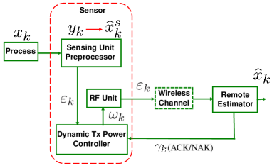
Figure 1: The system architecture.

2.1 Sensor Local Estimate

Hovareshti et al. [11] illustrated that utilization of the computation capabilities of wireless sensors may improve the system performance significantly. Equipped with such “smart sensors”, the sensor locally runs a Kalman filter to produce the MMSE estimate $\hat{x}_{k}^{s}$ of the state $x_{k}$ based on all the measurements collected up to time $k$, i.e., $y_{1:k}\triangleq\{y_{1},...,y_{k}\}$, and then transmits its local estimate to the remote estimator. Denote the sensor’s local MMSE state estimate, the corresponding estimation error and error covariance as $\hat{x}_{k}^{s}$, $e^{s}_{k}$ and $P_{k}^{s}$, respectively, i.e., $\hat{x}_{k}^{s}\triangleq\mathbb{E}[x_{k}|y_{1:k}]$, $e_{k}^{s}\triangleq x_{k}-\hat{x}_{k}^{s}$ and ${P}_{k}^{s}\triangleq\mathbb{E}[(x_{k}-\hat{x}_{k}^{s})(x_{k}-\hat{x}_{k}^{s})^{\prime}|y_{1:k}]$. Standard Kalman filtering analysis suggests that these quantities can be calculated recursively (cf., [12]), where the recursion starts from $\hat{x}_{0}^{s}=0$ and $P_{0}^{s}=\Pi_{0}\succeq 0$. Since $P_{k}^{s}$ converges to a steady-state value exponentially fast (cf., [12]), we assume that the sensor’s local Kalman filter has entered the steady state, that is, $P_{k}^{s}=\overline{P}\succeq 0~{}\forall k\in\mathbb{N}$, This assumption simplifies our subsequent analysis and results, such as Theorem 4.8 and Proposition 4.17.

2.2 Wireless Communication Model

The data are sent to the remote estimator over an Additive White Gaussian Noise (AWGN) channel using the Quadrature Amplitude Modulation (QAM) whereby $\hat{x}_{k}^{s}$ is quantized into $K$ bits and mapped to one of $2^{K}$ available QAM symbols. For simplicity, the following assumptions are made:

1. The channel noise is independent of $w_{k}$ and $v_{k}$.

2. $K$ is large enough so that quantization effect is negligible when analyzing the performance of the remote estimator.

3. The remote estimator can detect symbol errors. Only the data arriving error-free are regarded as being successfully received; otherwise they are regarded as dropout.

These assumptions are commonly used in communication and control theories (cf.,[13, 14, 4, 5, 8]). For example, Fu and Souza [14] demonstrated that the estimation quality improvement (in terms of reduction of the remote estimation error) achieved by increasing the number $K$ of the quantization bits is marginal when $K$ is sufficiently large (in their example $K$ only needs to be greater or equal to 4. Based on A.3, the communication channel can be characterized by a random process $\{\gamma_{k}\}_{k\in\mathbb{N}_{+}}$, where

$$\gamma_{k}=\begin{cases}1,&\text{if $\hat{x}^{s}_{k}$ arrives error-free at time $k$,}\\ 0,&\text{otherwise,}\end{cases}\vspace{-1mm}$$

initialized with $\gamma_{0}=1$. Denote $\gamma_{1:k}\triangleq\{\gamma_{1},\ldots,\gamma_{k}\}.$ Let $\omega_{k}\in[0,+\infty)$ be the transmission power for the QAM symbol at time $k$. We adopt the wireless communication channel model used in [10], and have ${\mathrm{Pr}}\left(\gamma_{k}=0|\omega_{k}\right)=q^{\omega_{k}},$ where $q$ is given by $q\triangleq\exp(-\alpha/({N_{0}W}))\in(0,1),$ $N_{0}$ is the AWGN noise power spectral density, $W$ is the channel bandwidth, and $\alpha\in(0,1]$ is a constant that depends on the specific modulation being used. To send local estimates to the remote estimator, the sensor chooses from a continuum of available power levels $\omega_{k}\geqslant 0$, see Fig. 1. Note that different power levels lead to different dropout rates, thereby affecting estimation performance.

2.3 Remote State Estimation

Define $\mathrm{I}_{k}$ as the information available to the remote estimator up to time $k$, i.e.,

$$\mathrm{I}_{k}=\{\gamma_{1}\hat{x}_{1}^{s},\gamma_{2}\hat{x}_{2}^{s},...,\gamma_{k}\hat{x}_{k}^{s}\}\cup\{\gamma_{1:k}\}.$$ (3)

Denote $\hat{x}_{k}$ and $P_{k}$ as the remote estimator’s own MMSE state estimate and the corresponding estimation error covariance, i.e., $\hat{x}_{k}\triangleq\mathbb{E}[x_{k}|\mathrm{I}_{k}]$ and ${P}_{k}\triangleq\mathbb{E}[(x_{k}-\hat{x}_{k})(x_{k}-\hat{x}_{k})^{\prime}|\mathrm{I}_{k}]$, where expectations are taken with respect to a fixed power controller. We assume that the remote estimator feedbacks acknowledgements $\gamma_{k}$ before time $k+1$. Such setups are common especially when the remote estimator (gateway) is an energy-abundant device. This energy asymmetry allows the estimator to trade energy cost for estimation accuracy.

3 Data-driven Transmission Power Control

Our strategy uses the measurements to assign transmission power level efficiently. As focusing on how the power controller utilize the sensor’s real-time data, to simplify discussion, we assume a constant power baseline $\bar{\omega}$ in this section. We define $\theta\triangleq\{\theta_{k}\}_{k\in\mathbb{N}_{+}}$ as a transmission power controller over the entire time horizon, where $\theta_{k}$ is a mapping from $y_{1:k}$ and $\gamma_{1:k}$ to $\omega_{k}$. Before proceeding to study $\theta$, let us first briefly explain the idea of data-driven power control mechanism. Define $\tau(k)\in\mathbb{N}_{+}$ as the holding time since the most recent time when the remote estimator received the data from the sensor, i.e.,

$$\tau(k)\triangleq k-\max_{1\leqslant t\leqslant k-1}\{t:\gamma_{t}=1\}.$$ (4)

We interchange $\tau(k)$ with $\tau$ when the underlying time index is clear from the context. Define $\varepsilon_{k}$ as the incremental innovation in the sensor local state estimate compared to time $k-\tau$, the previous reception instant, i.e.,

$$\varepsilon_{k}=\hat{x}_{k}^{s}-A^{\tau}\hat{x}_{k-\tau}^{s}.$$ (5)

Lemma 3.1.

$\mathbb{E}[e_{k}^{s}\varepsilon_{k}^{\prime}|\mathrm{I}_{k-1},\gamma_{k}=0]=0~{}\forall k\in\mathbb{N}_{+}.$ Proof: The result follows from noting that

$$\mathbb{E}[e_{k}^{s}\varepsilon_{k}^{\prime}|\mathrm{I}_{k-1},\gamma_{k}=0] = \mathbb{E}\left[\mathbb{E}[e_{k}^{s}\varepsilon_{k}^{\prime}|y_{1:k},\gamma_{1:k}]|\mathrm{I}_{k-1},\gamma_{k}=0\right]$$

$$= \mathbb{E}\left[\mathbb{E}[e_{k}^{s}|y_{1:k}]\varepsilon_{k}^{\prime}|\mathrm{I}_{k-1},\gamma_{k}=0\right]=0,$$

where the second equality holds because $e_{k}^{s}$ is independent of $\gamma_{1:k}$, and the last equality holds since $\mathbb{E}[e_{k}^{s}|y_{1:k}]=0.$

Note that, if $\varepsilon_{k}=0$, then the sensor generates a local estimate, $\hat{x}_{k}^{s}$ identical to the prediction $A^{\tau}\hat{x}_{k-\tau}^{s}$. We would say that, for the remote estimator, the “value” of information contained in $\hat{x}_{k}^{s}$ is null. As $\varepsilon_{k}$ becomes larger, $\hat{x}_{k}^{s}$ has an increasing drift from the prediction $A^{\tau}\hat{x}_{k-\tau}^{s}$ and the importance of the sensor sending $\hat{x}_{k}^{s}$ thereby raises. Motivated by these observations, we define a stationary power controller, $\theta_{\rm ef}:\varepsilon_{k}\rightarrow\omega_{k}$, as an increasing function of $\varepsilon_{k}$. To fit the above observations, we introduce a quadratic function of $\varepsilon_{k}$ given by $\mathcal{C}(\varepsilon_{k},\mathcal{Q})\triangleq{\varepsilon_{k}}^{\prime}\mathcal{Q}\varepsilon_{k},$ where $\mathcal{Q}\in\mathbb{S}_{+}^{n}$ is a weight matrix. According to Lemma 3.1, the covariance of $\varepsilon_{k}$ is a function of $\tau(k)$. Therefore we specify $\tau(k)$ for the index of $\mathcal{Q}$ and construct the following controller:

$$\theta_{\text{ef}}:\{\omega_{k}=\frac{N_{0}W}{2\alpha}\mathcal{C}(\varepsilon_{k},\mathcal{Q}_{\tau})+\omega\}.$$ (6)

In contrast to (6), most non-data-driven transmission power controllers (i.e., [4, 5]) use a given power $\bar{\omega}$ regardless of what value $\varepsilon_{k}$ takes. Note that in (6) a constant term $\omega$ is added after $\mathcal{C}(\varepsilon_{k},\mathcal{Q}_{\tau})$. If one sets $\mathcal{Q}_{\tau}=0$, then the transmission with the baseline power controller $\omega=\bar{\omega}$ is a special case of the proposed transmission power controller. As for $\mathcal{Q}_{\tau}\not=0$, the transmission power is a constant $\omega$ if $\mathcal{C}(\varepsilon_{k}\mathcal{Q}_{\tau})=0$; otherwise it is adapted according to $\mathcal{C}(\varepsilon_{k},\mathcal{Q}_{\tau})$. Compared with a related controller proposed earlier in [10], $\theta_{\text{ef}}$ in (6) is more general at least from two aspects: 1) we introduce a weight matrix $\mathcal{Q}_{\tau}$ to highlight the roles of different entries of $\varepsilon_{k}$; 2) it allows the sensor to transmit using a standard power $\omega$ even if $\mathcal{C}(\varepsilon_{k},\mathcal{Q}_{\tau})=0$, which includes a non-data-driven power transmission as a special case. As shown later in Lemma 4.4, given $\mathrm{I}_{k-1}$, $\varepsilon_{k}$ is zero-mean Gaussian with a covariance $\Sigma_{\tau}$ depending on $\tau(k)$, i.e., $(\varepsilon_{k}|\mathrm{I}_{k-1})\sim\mathcal{N}(0,\Sigma_{\tau}).$ For convenience of our subsequent analysis, we define a new parameter $\Psi_{\tau}$ satisfying $\Psi_{\tau}\triangleq\left(\mathcal{Q}_{k}+\Sigma_{\tau}^{-1}\right)^{-1},$ where $\Sigma_{\tau}\succeq\Psi_{\tau}\succeq 0$. We now list the main problems considered in the remainder of this work,

1. Under $\theta_{\rm ef}$ defined in (6), what is the MMSE estimate and its associated estimation error covariance?

2. What value should $\mathcal{Q}_{\tau}$ (or $\Psi_{\tau}$) take in order to minimize, $\mathbb{E}[P_{k}]$, the expected estimation error at the remote estimator?

The solution to the first problem is presented in Section 4.2. A sub-optimal solution to the second one is given in Section 4.3 in view of the difficulty of the optimization problem.

Before proceeding, we note that in previous works such as [8] the difficulty of using the information contained in lost packets, i.e., $\gamma_{k}=0$, when computing the MMSE estimate of the plant state has been acknowledged. One typically discards such information as was done in [8] or resorts to approximations, e.g., treating a truncated Gaussian distribution as a Gaussian distribution as was done in [15]. These approaches either lead to conservative results (due to the unutilized information) or inaccurate results (due to approximations). Our method, on other hand, makes use of the information contained in the event $\gamma_{k}=0$ to improve the estimation performance. The associated MMSE estimate, relying on no approximation techniques, is derived in a closed-form.

4 Main Results

4.1 Preliminaries

For any $\Sigma\succeq 0$ that is singular, there exist matrices $U,D\in\mathbb{R}^{n\times n}$ such that $\Sigma=UDU^{\prime},$ where $U$ is unitary, whose columns are right eigenvectors of $\Sigma$, and $D\triangleq\left[\begin{array}[]{cc}\Delta&0\\ 0&0\end{array}\right]$, where $\Delta$ is a diagonal matrix generated by the corresponding nonzero eigenvalues of $\Sigma$. Let $\Sigma^{1/2}\triangleq U\sqrt{D}$. Then $\Sigma=\Sigma^{1/2}\left(\Sigma^{1/2}\right)^{\prime}.$

Generally speaking, an $n$-dimensioned random vector $\mathbf{x}\sim\mathcal{N}(\mu,\Sigma)$, does not have a pdf with respect to the Lebesgue measure on $\mathbb{R}^{n}$ if some entries in $\mathbf{x}$ degenerate to almost surely constant random variables. To work with such vectors, one can instead consider Lebesgue measure in the $\mathrm{rank}(\Sigma)$-dimension affine subspace: $\Omega\triangleq\{\mu+\Sigma^{{1}/{2}}\mathbf{z}:~{}\mathbf{z}\in\mathbb{R}^{n}\}$, with respect to which $\mathbf{x}$ has a pdf $\mathrm{pdf}(\mathbf{x},x)=\frac{1}{\sqrt{\sigma}}\exp{\left(-\frac{1}{2}(x-\mu)^{\prime}\Sigma^{-1}(x-\mu)\right)},$ where $\sigma=(2\pi)^{\mathrm{rank}(\Sigma)}\mathrm{det}(\Sigma)$. Without loss of generality, in the remainder of this paper, for a random variable $\mathbf{x}\sim\mathcal{N}(0,\Sigma)$ with a singular $\Sigma$, the pdf of $\mathbf{x}$ means the probability density on $\Omega$. Note that the Moore-Penrose pseudoinverse of $\Sigma$ is unique and given by

$$\Sigma^{-1}=U\left[\begin{array}[]{lc}\Delta^{-1}&0\\ 0&0\end{array}\right]U^{\prime},$$ (7)

and that the pseudo-determinant of $\Sigma$ equals to the product of all nonzero eigenvalues of $\Sigma$.

Consider the power control law $\theta_{\rm ef}$ defined in (6). In order to guarantee that $\omega_{k}$ is always nonnegative for any value $\varepsilon_{k}$, the difference of $\Psi_{\tau}^{-1}$ and $\Sigma_{\tau}^{-1}$ needs to be at least positive semi-definite, i.e., two conditions must be simultaneously satisfied, which are $\Sigma_{\tau}\succeq\Psi_{\tau}$ and $\Psi_{\tau}^{-1}\succeq\Sigma_{\tau}^{-1}.$ The following lemma provides a necessary condition that $\Psi_{\tau}$ needs to satisfy.

Lemma 4.1.

Suppose $\Sigma$ and $\Psi$ satisfy $\Sigma\succeq\Psi$ and $\Psi^{-1}\succeq\Sigma^{-1}$. Then

$$\mathrm{rank}(\Psi)=\mathrm{rank}(\Sigma)$$ (8)

and

$$\mathrm{Im}(\Sigma^{{1}/{2}})=\mathrm{Im}(\Psi^{{1}/{2}}),$$ (9)

where $\mathrm{Im}(X)$ is the image of $X$. Proof: Since $\Sigma\succeq\Psi$, it is true that $\mathrm{rank}(\Sigma)\geq\mathrm{rank}(\Psi)$. To verify (8), suppose that $\mathrm{rank}(\Sigma)>\mathrm{rank}(\Psi)$. Then from (7), $\mathrm{rank}(\Sigma^{-1})>\mathrm{rank}(\Psi^{-1})$, which contradicts with $\Psi^{-1}\succeq\Sigma^{-1}$. To prove (9), let us denote $\mathrm{rank}(\Psi)\triangleq r$ and assume there is a set of vectors $\mathbf{W}\triangleq\{\mathbf{w}_{1},\ldots,\mathbf{w}_{r}\}$ such that $\mathrm{Im}(\Psi^{{1}/{2}})=\mathrm{span}\left(\{\mathbf{w}_{1},\ldots,\mathbf{w}_{r}\}\right).$ Suppose $\mathrm{Im}(\Sigma^{{1}/{2}})\neq\mathrm{Im}(\Psi^{{1}/{2}})$. Then there exists a vector in $\mathbf{W}$ (without loss of generality, let it be $\mathbf{w}_{1}$), and a vector $\mathbf{w}_{0}\in\mathrm{Ker}\left((\Sigma^{1/2})^{\prime}\right)$ where the operator $\mathrm{Ker}(X)$ is the kernel of a matrix $X$, such that ${\mathbf{w}_{0}}^{\prime}\mathbf{w}_{1}\neq 0$. It leads to the fact that $\mathbf{w}_{0}\not\in\mathrm{Ker}\left((\Psi^{1/2})^{\prime}\right)$. We in turn have

$${\mathbf{w}_{0}}^{\prime}\Sigma^{{1}/{2}}\left(\Sigma^{{1}/{2}}\right)^{\prime}\mathbf{w}_{0}=0\hbox{~{}~{}while~{}~{}}{\mathbf{w}_{0}}^{\prime}\Psi^{{1}/{2}}\left(\Psi^{{1}/{2}}\right)^{\prime}\mathbf{w}_{0}>0,$$

which contradicts with $\Sigma\succeq\Psi$.

For convenience, denote $n_{\tau}\triangleq\mathrm{rank}(\Sigma_{\tau})=\mathrm{rank}(\Psi_{\tau})$, $\Omega_{\tau}\triangleq\mathrm{Im}(\Sigma_{\tau}^{1/2})=\mathrm{Im}(\Psi_{\tau}^{1/2})$ and $\Phi_{\tau}\triangleq\left(\Sigma_{\tau}^{1/2}\right)^{\prime}\Psi_{\tau}^{-1}\Sigma_{\tau}^{1/2}.$ One has next lemma, the proof provided in the Appendix.

Lemma 4.2.

The rank of $\Phi_{\tau}$ equals that of $\Sigma_{\tau}$ (or $\Psi_{\tau}$), i.e., $\mathrm{rank}(\Phi_{\tau})=n_{\tau}.$

Example 4.3.

Two matrices are provided below as a simple example for $n=3$,

$$\Sigma_{\tau}=\left[\begin{array}[]{ccc}5&0&0\\ 0&5&0\\ 0&0&0\end{array}\right],\hbox{~{}~{}and~{}~{}}\Psi_{\tau}=\left[\begin{array}[]{ccc}3&-1&0\\ -1&3&0\\ 0&0&0\end{array}\right].$$

We can verify that $n_{\tau}=2$, $\Sigma_{\tau}\succeq\Psi_{\tau}$, $\Psi_{\tau}^{-1}\succeq\Sigma_{\tau}^{-1}$, (8), and Lemma 4.1 holds.

4.2 MMSE State Estimate

In general, the posterior distribution of $\varepsilon_{k}$ fails to maintain Gaussianity without analog-amplitude observations. The defect is especially common for quantized Kalman filtering and Gaussian filters, where it is tackled by Gaussian approximation [12, 16, 17]. By contrast, the following lemma shows that, using $\theta_{\rm ef}$ in (6), the distribution of $\varepsilon_{k}$ conditioned on $\mathrm{I}_{k-1},\gamma_{k}=0$ is Gaussian. The proof, similar to that of Lemma 3.5 in [10], is omitted.

Lemma 4.4.

Under $\theta_{\rm ef}$ defined in (6), given $\mathrm{I}_{k-1}$, $\varepsilon_{k}$ follows a Gaussian distribution: $(\varepsilon_{k}|{\mathrm{I}_{k-1}})\sim\mathcal{N}(0,{\Sigma_{\tau}}),$ where $\Sigma_{\tau}$ is given by the following recursion:

$$\Sigma_{\tau}=A\Psi_{\tau-1}A^{\prime}+\left(h(\overline{P})-\overline{P}\right),$$ (10)

with $\Psi_{0}=0$. It is also true that, given $\gamma_{k}=0$ and $\mathrm{I}_{k-1}$, $(\varepsilon_{k}|{\mathrm{I}_{k-1}},\gamma_{k}=0)\sim\mathcal{N}(0,{\Psi_{\tau}}).$

Proposition 4.5.

Under $\theta_{\rm ef}$ defined in (6), given $\mathrm{I}_{k-1}$, the packet drop rate at time $k$ is given by $\mathrm{Pr}(\gamma_{k}=0|\mathrm{I}_{k-1})=\frac{1}{\sqrt{\mathrm{det}(\Sigma_{\tau})\mathrm{det}(\Psi_{\tau}^{-1})}}\exp\left(-\frac{\alpha}{N_{0}W}\omega\right).$

We denote the packet arrival rate as $p_{\tau}\triangleq 1-\mathrm{Pr}(\gamma_{k}=0|\mathrm{I}_{k-1}),$ where the subscript $\tau$ is to emphasize that it depends on $\Sigma_{\tau}$ and $\Psi_{\tau}$. To ensure that the averaged transmission power with respect to different values taken by the measurement in $\theta$ does not exceed $\bar{\omega}$, i.e., $\mathbb{E}[\omega_{k}|\mathrm{I}_{k-1}]\leq\bar{\omega}$, we require the following result.

Lemma 4.6.

Under $\theta_{\rm ef}$ (6), given $\mathrm{I}_{k-1}$, the relation between $\mathbb{E}[\omega_{k}|\mathrm{I}_{k-1}]$ and $\Psi_{\tau}$, and $\omega$ is given by

$$\mathbb{E}[\omega_{k}|\mathrm{I}_{k-1}]=\frac{N_{0}W}{2\alpha}\left(\mathrm{Tr}(\Sigma_{\tau}\Psi_{\tau}^{-1})-{n_{\tau}}\right)+\omega.$$ (11)

Proof: From Lemma 4.4, we know that $(\varepsilon_{k}|{\mathrm{I}_{k-1}})\sim\mathcal{N}(0,{\Sigma_{\tau}}).$ Under $\theta_{\rm ef}$, we have:

$$\mathbb{E}[\omega_{k}|\mathrm{I}_{k-1}] = \mathbb{E}\left[\mathbb{E}[\omega_{k}|\varepsilon_{k}]|\mathrm{I}_{k-1}\right]$$

$$= \frac{N_{0}W}{2\alpha}\mathbb{E}\left[\varepsilon_{k}^{\prime}\left(\Psi_{\tau}^{-1}-\Sigma_{\tau}^{-1}\right)\varepsilon_{k}\right|\mathrm{I}_{k-1}]+\omega$$

$$= \frac{N_{0}W}{2\alpha}\mathrm{Tr}\left(\mathbb{E}\left[\varepsilon_{k}\varepsilon_{k}^{\prime}|\mathrm{I}_{k-1}\right](\Psi_{\tau}^{-1}-\Sigma_{\tau}^{-1})\right)+\omega$$

$$= \frac{N_{0}W}{2\alpha}\left(\mathrm{Tr}(\Sigma_{\tau}\Psi_{\tau}^{-1})-{n_{\tau}}\right)+\omega.$$

With $\theta_{\text{ef}}$ defined in (6), the remote estimator computes $x_{k}$ and $P_{k}$ according to the following two theorems.

Theorem 4.7.

Under $\theta_{\mathrm{ef}}$ (6), the remote estimator computes $\hat{x}_{k}$ as

$$\hat{x}_{k}=\left\{\begin{array}[]{ll}\hat{x}_{k}^{s},&\mathrm{if}~{}\gamma_{k}=1,\\ A^{\tau}\hat{x}_{k-\tau}^{s},&\mathrm{if}~{}\gamma_{k}=0,\end{array}\right.$$ (12)

where $\hat{x}_{k}^{s}$ is updated as $\hat{x}_{k}^{s}=A^{\tau}\hat{x}_{k-\tau}^{s}+\varepsilon_{k}$ when $\gamma_{k}=1$. Proof: When $\gamma_{k}=1$, the result is straightforward since $\hat{x}_{k}^{s}$ is the MMSE estimate of $x_{k}$ given $y_{1:k}$. Now consider $\gamma_{k}=0$. The tower rule gives

$$\mathbb{E}\left[x_{k}|\mathrm{I}_{k-1},\gamma_{k}=0\right] = \mathbb{E}\left[\mathbb{E}\left[x_{k}|y_{1:k},\gamma_{1:k}\right]|\mathrm{I}_{k-1},\gamma_{k}=0\right]$$

$$= \mathbb{E}\left[A^{\tau}\hat{x}_{k-\tau}^{s}+\varepsilon_{k}|\mathrm{I}_{k-1},\gamma_{k}=0\right]$$

$$= A^{\tau}\hat{x}_{k-\tau}^{s}+\mathbb{E}\left[\varepsilon_{k}|\mathrm{I}_{k-1},\gamma_{k}=0\right].$$

Lemma 4.4 leads to $\mathbb{E}\left[\varepsilon_{k}|\mathrm{I}_{k-1},\gamma_{k}=0\right]=0$.

Theorem 4.8.

Under $\theta_{\mathrm{ef}}$ (6), $P_{k}$ at the remote estimator is updated as

$$P_{k}=\left\{\begin{array}[]{ll}\overline{P},&\mathrm{if}~{}\gamma_{k}=1,\\ \overline{P}+\Psi_{\tau},&\mathrm{if}~{}\gamma_{k}=0.\end{array}\right.$$ (13)

Proof: When $\gamma_{k}=1$ the result is straightforward. We only prove the case when $\gamma_{k}=0$.

$$\mathbb{E}\left[(x_{k}-\hat{x}_{k})(x_{k}-\hat{x}_{k})^{\prime}|\mathrm{I}_{k-1},\gamma_{k}=0\right]$$

$$= \mathbb{E}\left[(x_{k}-A^{\tau}\hat{x}_{k-\tau}^{s})(x_{k}-A^{\tau}\hat{x}_{k-\tau}^{s})^{\prime}|\mathrm{I}_{k-1},\gamma_{k}=0\right]$$

$$= \mathbb{E}\left[\mathbb{E}\left[(e_{k}^{s}+\varepsilon_{k})(\cdot)^{\prime}|y_{1:k},\gamma_{1:k}\right]|\mathrm{I}_{k-1},\gamma_{k}=0\right]$$

$$= \mathbb{E}[(e_{k}^{s})(e_{k}^{s})^{\prime}|y_{1:k}]+\mathbb{E}\left[(\varepsilon_{k})(\varepsilon_{k})^{\prime}|\mathrm{I}_{k-1},\gamma_{k}=0\right]$$

$$= \overline{P}+\Psi_{\tau},$$

where the third equality is due to Lemma 3.1 and the last one is from Lemma 4.4.

Remark 4.9.

Under a baseline power controller with a constant power control $\bar{\omega}$, the remote estimator’s estimate still obeys the recursion (12); however, the estimation error covariance is updated differently: $P_{k}=\overline{P}$ when $\gamma_{k}=1$, and $P_{k}=h(P_{k-1})=\Sigma_{\tau}$ when $\gamma_{k}=0$). Note that although the obtained estimates under the two power controllers are the same, their different estimation error covariance matrices suggest different confident levels with which the remote estimator trusts the obtained estimate: with the data-driven power controller, it is more convinced that the obtained estimate is close to the real state while less convinced with a non-data-driven power controller.

4.3 Selection of Design Parameters

The performances of $\theta_{\rm ef}$ for different $\Psi_{\tau}$’s are difficult to compare in general. However, for $\Sigma_{\tau}$ and $\Psi_{\tau}$, there must exist a real number $\epsilon_{\tau}\in(0,1]$ such that $\Psi_{\tau}\preceq\epsilon_{\tau}\Sigma_{\tau}$ and $\Psi_{\tau}\not\preceq\epsilon\Sigma_{\tau},\forall~{}\epsilon<\epsilon_{\tau}$. Observe that

$$\Phi_{\tau}=\left(\Sigma_{\tau}^{1/2}\right)^{\prime}\Psi_{\tau}^{-1}\Sigma_{\tau}^{1/2}\succeq\frac{1}{\epsilon_{\tau}}\left[\begin{array}[]{cc}I_{n_{\tau}}&0\\ 0&0\end{array}\right],$$

which yields $\epsilon_{\tau}=\frac{1}{\lambda_{1}(\Phi_{\tau})}.$ In light of (10), we further have $\Psi_{\tau}\preceq\epsilon_{\tau}\Sigma_{\tau}=\epsilon_{\tau}\left(A\Psi_{\tau-1}A^{\prime}+\Sigma_{1}\right).$ According to Proposition 4.5, it can be seen given $\tau(k)=\tau$ that $\mathbb{E}[P_{k}|\tau(k)=\tau]$ has an upper bound: $\mathbb{E}[P_{k}|\tau(k)=\tau]\preceq\overline{P}+(1-p_{\tau})\epsilon_{\tau}\left(A\Psi_{\tau-1}A^{\prime}+\Sigma_{1}\right).$ Instead of minimizing $\mathbb{E}[P_{k}]$, we minimize its upper bound which is equivalent to minimize $(1-p_{\tau})\epsilon_{\tau}$. Iterating over time, one eventually needs to minimize $(1-p_{\tau})\epsilon_{\tau}$ for any $\tau(k)\in\mathbb{N}_{+}$ at any $k\in\mathbb{N}_{+}$. To this end, we propose to assign parameters of $\theta_{\rm ef}$ in (6) as the solution to the following optimization problem:

Problem 4.10.

$$\min_{\Psi_{\tau},\Sigma_{\tau},\omega}~{}~{}\frac{1}{\left(\mathrm{det}(\Sigma_{\tau})\mathrm{det}(\Psi_{\tau}^{-1})\right)^{1/2}\lambda_{1}(\Phi_{\tau})}\exp{\left[-\frac{\alpha}{N_{0}W}\omega\right]},$$

$$~{}~{}\,\mathrm{s.t.}~{}~{}~{}~{}~{}\frac{N_{0}W}{2\alpha}\left(\mathrm{Tr}(\Sigma_{\tau}\Psi_{\tau}^{-1})-n_{\tau}\right)+\omega\leq\bar{\omega}.$$

The constraint is imposed by (11). To solve Problem 4.10, we first note that $\mathrm{Tr}(\Sigma_{\tau}\Psi_{\tau}^{-1})=\mathrm{Tr}(\Phi_{\tau}).$ However, for any matrix $X,Y\in\mathbb{R}^{n\times n}$, $\mathrm{det}(XY)=\mathrm{det}(X)\mathrm{det}(Y)$ does not hold in general since $\mathrm{det}(X)$ means $X$’s pseudo-determinant (in case $X$ is singular). Fortunately, this property still holds for $\Sigma_{\tau}$ and $\Psi_{\tau}^{-1}$. The proof is given in the Appendix.

Lemma 4.11.

Suppose $\Sigma_{\tau}$ and $\Psi_{\tau}$ satisfy $\Sigma_{\tau}\succeq\Psi_{\tau}\succeq 0$ and $\Psi_{\tau}^{-1}\succeq\Sigma_{\tau}^{-1}$. Then $\mathrm{det}(\Sigma_{\tau})\mathrm{det}(\Psi_{\tau}^{-1})=\mathrm{det}(\Phi_{\tau}).$

From linear algebra, $\mathrm{det}(\Phi_{\tau})=\prod_{i=1}^{n_{\tau}}\lambda_{i}(\Phi_{\tau})$, and $\mathrm{Tr}(\Phi_{\tau})=\sum_{i=1}^{n_{\tau}}\lambda_{i}(\Phi_{\tau}).$ We simply write $\lambda_{i}(\Phi_{\tau})$ as $\lambda_{i}(\tau)$, and denote the nonzero eigenvalues of $\Phi_{\tau}$ by $\Lambda_{\tau}\triangleq[\,\lambda_{1}(\tau),\ldots,\lambda_{n_{\tau}}(\tau)\,]$. Then Problem 4.10 can be recast as

Problem 4.12.

$$\min_{\Lambda_{\tau},\omega} \frac{1}{\lambda_{1}(\tau)\prod_{i=1}^{n_{\tau}}\lambda_{i}(\tau)^{1/2}}\exp{\left[-\frac{\alpha}{N_{0}W}\omega\right]},$$ (14)

$$\mathrm{s.t.} \frac{N_{0}W}{2\alpha}\left[\sum_{i=1}^{n_{\tau}}\lambda_{i}(\tau)-n_{\tau}\right]+\omega=\bar{\omega},~{}\omega\geq 0$$

$$1\leq\lambda_{1}(\tau)\leq\lambda_{j}(\tau),~{}\forall j=2,\ldots,n_{\tau}.$$

Lemma 4.13.

Let $\Lambda_{\tau}^{*}$ be the optimal solution to Problem 4.12. Then $\Lambda_{\tau}^{*}$ satisfies

$$\lambda_{1}(\tau)^{*}=\lambda_{2}(\tau)^{*}=\cdots=\lambda_{n_{\tau}}(\tau)^{*}.$$ (15)

Proof: Suppose that $\Lambda$ is the optimal solution to Problem 4.12 but does not satisfy (15). We will show that there must exist another vector, which is different from $\Lambda$ and has a smaller cost function (14). Let $\sum_{i=1}^{n_{\tau}}\lambda_{i}=c$ where $c$ is a positive constant. Due to the fact that $\lambda_{1}$ in $\Lambda$ is the minimum eigenvalue of $\Phi_{\tau}$ and the inequality of arithmetic and geometric means, we have $\lambda_{1}\leq\frac{c}{n_{\tau}}$ and $\prod_{i=1}^{n_{\tau}}\lambda_{i}\leq\left(\frac{c}{n_{\tau}}\right)^{n_{\tau}},$ the equalities simultaneously satisfied when $\lambda_{i}=\frac{c}{n_{\tau}},~{}\forall~{}i=1,\ldots,n_{\tau}$. Thus, $\Lambda_{0}=[{\frac{c}{n_{\tau}},\ldots,\frac{c}{n_{\tau}}}]$ results in a smaller value of (14), which contradicts with the assumption and completes the proof.

The following lemma is a result of Lemma 4.13. Its proof is presented in the Appendix.

Lemma 4.14.

If $\bar{\omega}>\frac{N_{0}W}{\alpha}$, then the optimal solution to Problem 4.12 is $\omega=\bar{\omega}-\frac{N_{0}W}{\alpha}$ and

$$\Lambda_{\tau}^{*}=[1+\frac{2}{n_{\tau}},\ldots,1+\frac{2}{n_{\tau}}].$$ (16)

Otherwise, if $\bar{\omega}\leq\frac{N_{0}W}{\alpha}$, the optimizer is $\omega=0$ and

$$\Lambda_{\tau}^{*}=[1+\frac{2\alpha\bar{\omega}}{n_{\tau}N_{0}W},\ldots,1+\frac{2\alpha\bar{\omega}}{n_{\tau}N_{0}W}].$$ (17)

Denote by $\theta_{\rm ef}^{*}$ the transmission power associated with the solution to Problem 4.12. Then we have the following theorem. It can be readily verified from Lemma 4.14.

Theorem 4.15.

If $\bar{\omega}>\frac{N_{0}W}{\alpha}$, then $\theta_{\rm ef}^{*}$ is given by

$$\theta_{\rm ef}^{*}:~{}\{\omega_{k}=\frac{N_{0}W}{\alpha n_{\tau}}\varepsilon_{k}^{\prime}\Sigma_{\tau}^{-1}\varepsilon_{k}+\bar{\omega}-\frac{N_{0}W}{\alpha}\},$$

where $\Sigma_{\tau+1}=\frac{n_{\tau}}{n_{\tau}+2}A\Sigma_{\tau}A^{\prime}+h(\overline{P})-\overline{P}$ with $\Sigma_{0}=0$. Otherwise, if $\bar{\omega}\leq\frac{N_{0}W}{\alpha},$ $\theta_{\rm ef}^{*}$ is given by

$$\theta_{\rm ef}^{*}:~{}\{\omega_{k}=\frac{\bar{\omega}}{n_{\tau}}\varepsilon_{k}^{\prime}\Sigma_{\tau}^{-1}\varepsilon_{k}\},$$

where $\Sigma_{\tau+1}=\frac{n_{\tau}N_{0}W}{n_{\tau}N_{0}W+2\alpha\bar{\omega}}A\Sigma_{\tau}A^{\prime}+h(\overline{P})-\overline{P}$.

Remark 4.16.

A non-data-driven baseline power controller with a constant power level $\bar{\omega}$ is feasible to Problem 4.10. Since $\theta_{\rm ef}^{*}$ is the optimal solution, it has not worse state estimation performance compared with the alternative non-data-driven power controller. Numerical examples in Section 5 demonstrate performance improvements using $\theta_{\rm ef}^{*}$ compared with the non-data-driven power controller.

The following proposition shows that the rank of $\Sigma_{\tau}$ can be calculated offline. The proof is given in the Appendix.

Proposition 4.17.

Consider the $\theta_{\rm ef}^{*}$ given in Theorem 4.15, for any $\tau\in\mathbb{N}_{+}$, $n_{\tau}$ can be calculated as: $n_{\tau}=\mathrm{rank}(h^{\tau}(\overline{P})-\overline{P}).$ In particular, when $\tau\geq n$, the dimension of $x$, $n_{\tau}$ becomes a constant which is given by: $n_{\tau}=\mathrm{rank}(h^{n}(\overline{P})-\overline{P}),~{}\forall~{}\tau\geq n.$

4.4 Extension

In many cases, the base-line power controller changes over time with respect to different settings. For example, in [4], block fading channels were taken into account. To deal with a time-varying channel power gain $h_{k}$, a predictive power control algorithm was established, which determines the transmission power level, bit rates and codebooks used by the sensors. The algorithm in [4] requires that the receiver (i.e, the remote estimator) runs a channel gain predictor, see e.g., [18]. A key observation is that the data-driven controller proposed in the present work can be readily adapted to situations where the baseline controller provides time-varying power levels $\bar{w}_{k}$. In fact, by solving Problem 4.12 for a time-varying power baseline $\bar{\omega}_{k}$, we obtain the optimal solution $\theta_{\rm ef}^{*}$ as follows: If $\bar{\omega}_{k}>\frac{N_{0}W}{\alpha}$, then $\theta_{\rm ef}^{*}$ is given by

$$\theta_{\rm ef}^{*}:~{}\{\omega_{k}=\frac{N_{0}W}{\alpha n_{\tau}}\varepsilon_{k}^{\prime}\Sigma_{k}^{-1}\varepsilon_{k}+\bar{\omega}_{k}-\frac{N_{0}W}{\alpha}\}$$

and $\Psi_{k}=\frac{n_{\tau}}{n_{\tau}+2}\Sigma_{k-1}$. Otherwise, if $\bar{\omega}_{k}\leq\frac{N_{0}W}{\alpha},$ $\theta_{\rm ef}^{*}$ is given by

$$\theta_{\rm ef}^{*}:~{}\{\omega_{k}=\frac{\bar{\omega}}{n_{\tau}}\varepsilon_{k}^{\prime}\Sigma_{k}^{-1}\varepsilon_{k}\}$$

and $\Psi_{k}=\frac{n_{\tau}N_{0}W}{n_{\tau}N_{0}W+2\alpha\bar{\omega}}\Sigma_{k}.$ In both cases, $\Sigma_{k}=(1-\gamma_{k-1})A\Psi_{k-1}A^{\prime}+h(\overline{P})-\overline{P}$. Note that $\Sigma_{k}$, $\Psi_{k}$ and $\Phi_{k}$ are calculated similar to $\Sigma_{\tau}$, $\Psi_{\tau}$ and $\Phi_{\tau}$ given in Theorem 4.15. To reduce the sensor’s computational load, the sensor only needs to calculate the quadratic form $\varepsilon_{k}^{\prime}\Sigma_{\tau}^{-1}\varepsilon_{k}$, while the rest of the paraments are updated and then sent to the sensor by the estimator. Note that calculating $\varepsilon_{k}^{\prime}\Sigma_{\tau}^{-1}\varepsilon_{k}$ has a complexity of $O(n^{2})$.

5 Simulation and Examples

Consider a system with parameters as follows: $A=\left[\begin{array}[]{cc}0.99&0.3\\ 0.1&0.7\\ \end{array}\right],C=\left[\begin{array}[]{cc}2.3&1\\ 1&1.8\\ \end{array}\right],R=Q=I_{2\times 2}.$ We first assume that $\theta$ has a constant power baseline $\bar{\omega}=5$ and $\frac{N_{0}W}{\alpha}=3<\bar{\omega}.$ In Section 5.2, a time-varying power baseline is considered.

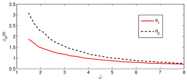
Figure 2: Empirical estimation covariance provided by controllers $\theta^{*}_{\text{ef}}(\theta_{1})$ and $\theta_{2}$ as a function of energy constraint $\bar{\omega}$.

5.1 Comparison with Different Energy Constraints

We compare our proposed schedule $\theta_{\rm ef}^{*}$ (denoted as $\theta_{1}$) with a constant baseline power controller within the entire time horizon (denoted as $\theta_{2}:\{\omega_{k}=\bar{\omega}\}$). Define $J_{k}(\theta)=\frac{1}{k}\sum_{i=1}^{k}\mathrm{Tr}\left(\mathbb{E}[P_{i}]\right)$ as the empirical approximation (via 100000 Monte Carlo simulations) of the average expected state error covariance (denoted as $J(\theta)$). We choose $J_{30}(\theta)$ as an approximation of $J(\theta)$.

Fig. 2 shows that $\theta_{\rm ef}^{*}$ leads to a better system performance when compared to $\theta_{2}$ under the same energy constraint.

5.2 Comparison under Fading Channels

In practice, wireless communication channels typically comprise fading often assumed to be Rayleigh [19], i.e., the channel power gain $h_{k}$ is exponentially distributed with $\mathrm{pdf}(h_{k})=\frac{1}{\overline{h}}\exp{(-\frac{h_{k}}{\overline{h}})},$ where $h_{k}\geqslant 0$ and $\overline{h}$ is the mean of $h_{k}$. Truncated channel inversion transmit power controllers have been studied in several works [7, 5, 20], where the transmission power is the inversion of $h_{k}$, with a truncated boundary. In this subsection, we use the baseline power determined by truncated channel gain inversion Denote the truncated channel inversion transmission power controller as $\theta_{3}$:

$$\omega_{k}=\left\{\begin{array}[]{ll}\frac{v}{h_{k}},&h_{k}>h^{\star},\\ \frac{v}{h^{\star}},&\mathrm{otherwise}.\end{array}\right.$$ (18)

where $v$ and $h^{\star}$ are design parameters. Consider the case of $\overline{h}=1$ and set $h^{\star}=5$. Based on the results in [5], we can choose $v$ to meet the energy constraint. Fig. 3 suggests that $\theta_{\rm ef}^{*}$ leads to better system performance when compared with $\theta_{3}$. Fig. 4 shows the comparison given a specific realization of channel power gains.

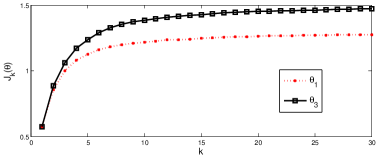
Figure 3: Comparison of $\theta^{*}_{\text{ef}}(\theta_{1})$ and $\theta_{3}$ under Rayleigh fading.

Figure 4: Comparison of $\theta^{*}_{\text{ef}}(\theta_{1})$ and $\theta_{3}$ given a specific realization of channel power gains.

6 Conclusion

We proposed a data-driven transmission power controller for remote state estimation, which adjusts the sensor’s transmission power according to its real-time measurements. Then we proved that the proposed power controller preserves Gaussianity of the incremental innovation and provided a closed-form expression of the expected state estimation error covariance. a tuning method for parameter design was presented to guarantee that the data-driven power controller not worse performance than the alternative non-data-driven ones. Comparisons were conducted to illustrate estimation performance improvement.

Appendix

Proof of Lemma 4.2:  To verify the clain, it suffices to show that $\mathrm{rank}(\Phi_{\tau})\geq n_{\tau}$. Suppose that $\mathrm{rank}(\Phi_{\tau})=r<n_{\tau}$. Since $\Phi_{\tau}\succeq 0$, there must exist exactly $n-r$ mutually orthogonal vectors $\mathbf{e}_{1},\ldots,\mathbf{e}_{n-r}$ such that ${\mathbf{e}_{i}}^{\prime}\Phi_{\tau}\mathbf{e}_{i}=0,\hbox{~{}for~{}}i=1,\ldots,n-r.$ Denote the unit vector with only the $(n_{\tau}+j)$th entry being $1$ by $\mathbf{i}_{j}$, that is, $\mathbf{i}_{j}=[\,\underbrace{0,\ldots,0,1}_{n_{\tau}+j},0,\ldots,0\,]^{\prime}.$ Since ${\mathbf{i}_{j}}^{\prime}\Phi_{\tau}\mathbf{i}_{j}=0,~{}j=1,\ldots,n-n_{\tau},$ without loss of generality, let $\mathbf{e}_{j}=\mathbf{i}_{j}$. As we assume that $\mathbf{e}_{n-r}$ is orthogonal to $\mathbf{e}_{j},~{}j=1,\ldots,n-n_{\tau},$ it is true that $D_{\tau}^{1/2}\mathbf{e}_{n-r}\neq 0$. Since $U_{\tau}$ is nonsingular and $\mathrm{Ker}(U_{\tau})=\{0\}$, we have $\mathbf{e}\triangleq\Sigma_{\tau}^{1/2}\mathbf{e}_{n-r}\neq 0$. We then observe that $\mathbf{e}^{\prime}\Psi_{\tau}^{-1}\mathbf{e}={\mathbf{e}_{n-r}}^{\prime}\Phi_{\tau}\mathbf{e}_{n-r}=0,$ and $\mathbf{e}^{\prime}\Sigma_{\tau}^{-1}\mathbf{e}={\mathbf{e}_{n-r}}^{\prime}\left[\begin{array}[]{cc}I_{n_{\tau}}&0\\ 0&0\end{array}\right]\mathbf{e}_{n-r}>0,$ which contradicts with $\Psi_{\tau}^{-1}\succeq\Sigma_{\tau}^{-1}$. $\blacksquare$

Proof of Lemma 4.11:  By definition, it is easy to see that $\mathrm{det}(\Sigma_{\tau})\mathrm{det}(\Psi_{\tau}^{-1})=\prod_{i=1}^{n_{\tau}}\lambda_{i}(\Sigma_{\tau}){\lambda_{i}(\Psi_{\tau})}^{-1}.$ Therefore we only need to prove $\mathrm{det}(\Phi_{\tau})=\prod_{i=1}^{n_{\tau}}\lambda_{i}(\Sigma_{\tau}){\lambda_{i}(\Psi_{\tau})}^{-1}.$ Observe that $\Sigma_{\tau}$ and $\Psi_{\tau}$ can be factorized as $\Sigma_{\tau}=U_{\tau}\left[\begin{array}[]{cc}\Delta_{\tau}&0\\ 0&0\end{array}\right]{U_{\tau}}^{\prime}$ and $\Psi_{\tau}=V_{\tau}\left[\begin{array}[]{cc}\Theta_{\tau}&0\\ 0&0\end{array}\right]{V_{\tau}}^{\prime}$, where $\Delta_{\tau}$ and $\Theta_{\tau}$ are diagonal matrices generated respectively by the nonzero eigenvalues of $\Sigma_{\tau}$ and $\Psi_{\tau}$. For $i=1,\ldots,n_{\tau}$, $u_{i}$ and $v_{i}$ are the eigenvectors associated with $\lambda_{i}(\Sigma_{\tau})$ and $\lambda_{i}(\Psi_{\tau})$. In addition, $U_{\tau}=[\,{u}_{1},\ldots,{u}_{n_{\tau}},{0},\ldots,{0}\,]$ and $V_{\tau}=[\,{v}_{1},\ldots,{v}_{n_{\tau}},{0},\ldots,{0}\,]$. Then $\Phi_{\tau}$ can be written as $\Phi_{\tau}=\left[\begin{array}[]{cc}M_{\tau}&0\\ 0&0\end{array}\right],$ where $M_{\tau}={\Delta_{\tau}}^{1/2}{\tilde{U}_{\tau}}^{\prime}\tilde{V}_{\tau}{\Theta_{\tau}}^{-1}{\tilde{V}_{\tau}}^{\prime}\tilde{U}_{\tau}{\Delta_{\tau}}^{1/2}\in\mathbb{S}_{+}^{n_{\tau}}$, $\tilde{U}_{\tau}=[\,u_{1},\ldots,u_{n_{\tau}}]$ and $\tilde{V}_{\tau}=[\,v_{1},\ldots,v_{n_{\tau}}]$. According to Lemma 4.3, $M_{\tau}$ is nonsingular, so $\mathrm{det}(\Phi_{\tau})=\mathrm{det}(M_{\tau})$. Since $\mathrm{Im}(\Sigma_{\tau})=\mathrm{Im}(\Psi_{\tau})$ from (9), there exists a unitary matrix $V$ such that $\tilde{V}_{\tau}=\tilde{U}_{\tau}V$. Thus, $\mathrm{det}(M_{\tau})=\mathrm{det}\left({\Delta_{\tau}}^{1/2}V{\Theta_{\tau}}^{-1}V^{\prime}{\Delta_{\tau}}^{1/2}\right)=\mathrm{det}\left({\Delta_{\tau}}{\Theta_{\tau}}^{-1}\right),$ which completes the proof. $\blacksquare$

Proof of Lemma 4.14:  According to Lemma 4.13, we set $\lambda_{1}(\tau)=\cdots=\lambda_{n_{\tau}}(\tau)=\lambda_{\tau}$. Logarithm does not change the monotonicity of (14). Problem 4.12 is consequently transformed to

$$\min\limits_{\lambda_{\tau},\omega} -\frac{\alpha}{N_{0}W}\omega-(\frac{n_{\tau}}{2}+1)\ln{\lambda_{\tau}},$$

s.t. $$\frac{n_{\tau}N_{0}W}{2\alpha}(\lambda_{\tau}-1)+\omega=\bar{\omega},~{}~{}\omega\geq 0.$$

Substituting $\omega=-\frac{\alpha}{N_{0}W}\bar{\omega}+\frac{n_{\tau}}{2}(\lambda_{\tau}-1)-(\frac{n_{\tau}}{2}+1)\ln{\lambda_{\tau}}$ into  (Appendix) and taking derivative, it yields that the minimum of (Appendix) is attained at $\lambda_{\tau}=1+\frac{2}{n_{\tau}}$. Meanwhile $\omega$ needs to be nonnegative, so the optimal solution to Problem 4.10 is (16) if $\bar{\omega}>\frac{N_{0}W}{\alpha}$ or (17) otherwise. $\blacksquare$

Proof of Proposition 4.17:  Consider a matrix $\Sigma=\sum_{i=1}^{\tau}\rho_{i}\left(h^{i}(\overline{P})-h^{i-1}(\overline{P})\right)$ with $\rho_{i}\in(0,1]$. We have

$$\mathrm{Im}(\Sigma) = \mathrm{Im}([\,\rho_{1}\Sigma_{1}^{1/2}~{}\rho_{2}A\Sigma_{1}^{1/2}~{}\cdots~{}\rho_{\tau}A^{\tau-1}\Sigma_{1}^{1/2}\,][\,\cdot\,]^{\prime})$$ (20)

$$= \mathrm{Im}([\,\rho_{1}\Sigma_{1}^{1/2}~{}\rho_{2}A\Sigma_{1}^{1/2}~{}\cdots~{}\rho_{\tau}A^{\tau-1}\Sigma_{1}^{1/2}\,])$$

$$= \mathrm{Im}([\,\Sigma_{1}^{1/2}~{}A\Sigma_{1}^{1/2}~{}\cdots~{}A^{\tau-1}\Sigma_{1}^{1/2}\,])$$

$$= \mathrm{Im}([\,\Sigma_{1}^{1/2}~{}A\Sigma_{1}^{1/2}~{}\cdots~{}A^{\tau-1}\Sigma_{1}^{1/2}\,][\,\cdot\,]^{\prime})$$

$$= \mathrm{Im}(h^{\tau}(\overline{P})-\overline{P}),$$

which leads to the first assertion. By the Cayley-Hamilton theorem, we have $A^{k}=-a_{1}(k)A^{n-1}-a_{2}(k)A^{n-2}-\cdots-a_{n}(k)I,~{}~{}\forall~{}k\geq n,$ where $a_{1}(k),\ldots,a_{n}(k)$ are coefficients of the characteristic polynomial of $A$. When $\tau\geq n+1$, we have

$$\mathrm{Im}([\,\Sigma_{1}^{1/2}~{}A\Sigma_{1}^{1/2}~{}\cdots~{}A^{\tau-1}\Sigma_{1}^{1/2}\,][\,\cdot\,]^{\prime})$$

$$= \mathrm{Im}([\,\Sigma_{1}^{1/2}~{}A\Sigma_{1}^{1/2}~{}\cdots~{}-a_{1}(\tau-1)A^{n-1}\Sigma_{1}^{1/2}$$

$$\;\;\;\;\;\;\;-a_{2}(\tau-1)A^{n-2}\Sigma_{1}^{1/2}-\cdots-a_{n}(\tau-1)\Sigma_{1}^{1/2}\,]),$$

The last assertion follows from the reasoning used in (20). $\blacksquare$

References

- [1] L. Shi and L. Xie, “Optimal sensor power scheduling for state estimation of Gauss–Markov systems over a packet-dropping network,” IEEE Transactions on Signal Processing, vol. 60, no. 5, pp. 2701–2705, 2012.
- [2] Y. Xu and J. P. Hespanha, “Optimal communication logics in networked control systems,” in Proceedings of the 43rd IEEE Conference on Decision and Control, vol. 4. IEEE, 2004, pp. 3527–3532.
- [3] O. C. Imer and T. Basar, “Optimal estimation with limited measurements,” in Proceedings of the 44th IEEE Conference on Decision and Control, European Control, December 2005, pp. 1029–1034.
- [4] D. E. Quevedo, A. Ahlén, and J. Østergaard, “Energy efficient state estimation with wireless sensors through the use of predictive power control and coding,” IEEE Transactions Signal Processing, vol. 58, no. 9, pp. 4811–4823, 2010.
- [5] A. S. Leong and S. Dey, “Power allocation for error covariance minimization in Kalman filtering over packet dropping links,” in Decision and Control (CDC), 2012 IEEE 51st Annual Conference on. IEEE, 2012, pp. 3335–3340.
- [6] M. Nourian, A. Leong, S. Dey, and D. E. Quevedo, “An optimal transmission strategy for Kalman filtering over packet dropping links with imperfect acknowledgements,” IEEE Trans. Contr. Network Syst., vol. 1, no. 3, pp. 259–271, Sept. 2014.
- [7] D. E. Quevedo, A. Ahlén, A. S. Leong, and S. Dey, “On Kalman filtering over fading wireless channels with controlled transmission powers,” Automatica, vol. 48, no. 7, pp. 1306–1316, 2012.
- [8] K. Gatsis, A. Ribeiro, and G. J. Pappas, “Optimal power management in wireless control systems,” in American Control Conference (ACC), 2013, 2013, pp. 1562–1569.
- [9] G. E. Box and G. C. Tiao, Bayesian inference in statistical analysis. Wiley-Interscience, 2011.
- [10] Y. Li, D. E. Quevedo, V. Lau, and L. Shi, “Online sensor transmission power schedule for remote state estimation,” in Proceedings of 52nd IEEE Conference on Decision and Control, Florence, Italy, 2013.
- [11] P. Hovareshti, V. Gupta, and J. S. Baras, “Sensor scheduling using smart sensors,” in Proceedings of the 46th IEEE Conference on Decision and Control, 2007, pp. 494–499.
- [12] B. D. O. Anderson and J. Moore, Optimal Filtering. Englewood Cliffs, NJ: Prentice Hall, 1979.
- [13] B. Sinopoli, L. Schenato, M. Franceschetti, K. Poolla, M. I. Jordan, and S. S. Sastry, “Kalman filtering with intermittent observations,” IEEE Transactions on Automatic Control, vol. 49, no. 9, pp. 1453–1464, 2004.
- [14] M. Fu and C. E. de Souza, “State estimation for linear discrete-time systems using quantized measurements,” Automatica, vol. 45, no. 12, pp. 2937 – 2945, 2009.
- [15] J. Wu, Q. shan Jia, K. H. Johansson, and L. Shi, “Event-based sensor data scheduling: Trade-off between communication rate and estimation quality,” IEEE Transactions on Automatic Control, vol. 58, no. 4, pp. 1041–1046, 2013.
- [16] J. H. Kotecha and P. M. Djuric, “Gaussian particle filtering,” IEEE Transactions on Signal Processing, vol. 51, no. 10, pp. 2592–2601, 2003.
- [17] A. Ribeiro, G. B. Giannakis, and S. I. Roumeliotis, “-: Distributed alman filtering with low-cost communications using the sign of innovations,” IEEE Transactions on Signal Processing, vol. 54, no. 12, pp. 4782–4795, 2006.
- [18] L. Lindbom, A. Ahlén, M. Sternad, and M. Falkenström, “Tracking of time-varying mobile radio channels–part II: A case study,” IEEE Transactions Commun., vol. 50, no. 1, pp. 156–167, Jan. 2002.
- [19] T. S. Rappaport et al., Wireless communications: principles and practice. Prentice Hall PTR New Jersey, 1996, vol. 2.
- [20] A. J. Goldsmith and P. P. Varaiya, “Capacity of fading channels with channel side information,” IEEE Transactions on Information Theory, vol. 43, no. 6, pp. 1986–1992, 1997.