Polymer quantization, stability and higher-order time derivative terms

Abstract

The possibility that fundamental discreteness implicit in a quantum gravity theory may act as a natural regulator for ultraviolet singularities arising in quantum field theory has been intensively studied. Here, along the same expectations, we investigate whether a nonstandard representation, called polymer representation can smooth away the large amount of negative energy that afflicts the Hamiltonians of higher-order time derivative theories; rendering the theory unstable when interactions come into play. We focus on the fourth-order Pais-Uhlenbeck model which can be reexpressed as the sum of two decoupled harmonic oscillators one producing positive energy and the other negative energy. As expected, the Schrödinger quantization of such model leads to the stability problem or to negative norm states called ghosts. Within the framework of polymer quantization we show the existence of new regions where the Hamiltonian can be defined well bounded from below.

I Introduction

The standard model of particles has foundations on local quantum field theories having operators of mass dimension $d\leq 4$. These operators are justified in order to implement the requirements of stability and unitarity without further elaborations eliezer . However, when going to higher energies it is commonly believed that higher-order operators will play a key role in describing fundamental physics. This may be particularly true when they involve higher time derivatives since the new modes that arise allow to describe effects from a high scale. Usually these new modes are very high when the coupling of the higher-order time derivatives are suppressed by the high scale as taken in effective approaches. Higher-order operators have received increased attention over the years. They have been investigated in the context of loop quantum gravity Gambini ; Alfaro ; Alfaro1 ; Alfaro2 ; Sahlmann ; Sahlmann1 , Lorentz symmetry violation KM1 ; KM2 ; KM3 ; MP ; schreck ; schreck1 , causality and stability reyescausality , fine-tuning large ; Reyes ; Reyes1 ; Reyes2 , the hierarchy problem Grinstein ; Grinstein1 , radiative corrections radcorr ; radcorr1 ; radcorr2 and nonminimal couplings casana-manoel ; casana-manoel1 ; casana-manoel2 ; casana-manoel3 ; petrov ; petrov1 . The presence of higher-order derivatives in the gravitational sector are a key ingredient in order to achieve a consistent renormalization in the semiclassical approach, where matter fields are quantized over classical curved background HD-grav .

Higher time derivative theories were introduced long time ago by Ostrogradsky OSTRO . The approach is based on a variational formalism and involves a Lagrangian $L(x,\dot{x},\ddot{x}\dots,x^{(n)}=\frac{d^{n}x}{dt^{n}})$ and an extended Hamiltonian $H(x,\pi_{\dot{x}},\pi_{\ddot{x}}\dots,\pi_{x^{(n)}})$ of $2n$ variables. Ostrogradsky showed that the formalism leads a higher-order Hamiltonian not bounded from below as can be seen in the non-quadratic momenta terms that appear. This is the classical Ostrogradsky instability of higher-order time derivative theories which can be avoided in a few cases, for instance when the models has constraints mijael .

The quantization of higher time derivative theories can be implemented introducing a change of variables in order to transform the original Lagrangian into a sum of decoupled normal-order Lagrangians. In general one of these Lagrangians has large negative energy leading to the instability or alternatively, by changing the vacuum state, to an indefinite metric theory P-U . The instability of the Hamiltonian has received much attention and has been tackled from different perspectives, such as phase space reduction cheng ; cheng1 ; pert , complex canonical transformations hugo , $\mathcal{PT}$ symmetry PT ; PT1 ; PT2 , and Euclidean-path reduced amplitudes hawkings , gravitational ghosts and tachyons grav-ghosts ; grav-ghosts1 . In quantum field theory, Lee and Wick showed that by imposing the negative norm states to decay it is possible to preserve unitarity order by order in perturbation theory L-W ; L-W1 . Resurgence of such ideas have been used to solve the hierarchy problem Grinstein ; Grinstein1 and in higher-order effective models with Lorentz symmetry violation unit ; unit1 ; unit2 .

In this work we study the stability of higher-order time derivative models within the framework of polymer quantization. In particular, we focus on the Pais-Uhlenbeck (P-U) model. The polymer representation is a non-standard representation of quantum mechanics inspired by some results that emerge from loop quantum gravity. The possibility of space discreteness that appears in loop quantum gravity ash has served to improve the convergence of quantum field theories Sahlmann ; Sahlmann1 and cosmological singularities Bojowald . In this paper our main goal is to test whether the fundamental discreteness implicit in the polymer representation allows to improve the stability of higher-order theories. The polymer quantization has been considered in several studies such as two-point functions propagators ; propagators1 ; propagators2 , cosmology Bojowald ; tomasz , central forces r ; r1 , higher space derivatives martin , thermodynamics Chacon , compact stars Chacon-Acosta and low energy limits corichi ; corichi1 .

The organization of this work is as follows. In section II we introduce the P-U model and we explicitly show the origin of the instability in the Schrödinger quantization. In the third section we give a basic review of the polymer formalism. In section IV we polymer quantize the P-U model and solve the Hamiltonian eigenvalue equation. From the previous results we analyze stability in the region of validity of the theory. In the last section we give the conclusions.

II The Pais-Uhlenbeck model

The P-U model consists of an harmonic oscillator coupled to a higher-order term described by the Lagrangian

$$L=\frac{1}{2}m\dot{x}^{2}-\frac{1}{2}kx^{2}-\frac{g}{2}\ddot{x}^{2}\;,$$ (1)

where $g$ is a small parameter. The equation of motion is

$$-kx-m\frac{d^{2}x}{dt^{2}}-g\frac{d^{4}x}{dt^{4}}=0\;.$$ (2)

Inserting the plane wave ansatz $x(t)=x_{0}e^{-iyt}$ produces the four solutions

$$y=\pm\sqrt{\frac{m\pm\sqrt{m^{2}-4kg}}{2g}}\;.$$ (3)

We define the two positive solutions according to

$$\omega_{1}=\omega_{0}\sqrt{\frac{1-\sqrt{1-4\varepsilon}}{2\varepsilon}}\;,\quad\omega_{2}=\omega_{0}\sqrt{\frac{1+\sqrt{1-4\varepsilon}}{2\varepsilon}}\;,$$ (4)

where we introduce $\omega_{0}=\sqrt{k/m}$ as the usual frequency and $g=\frac{m\varepsilon}{\omega_{0}^{2}}$ with $\varepsilon$ a small dimensionless parameter. Now, in the limit $\varepsilon\to 0$ the first solution tends to the usual harmonic solution $\omega_{1}\to\omega_{0}$ and the second one $\omega_{2}\to\frac{\omega_{0}}{\sqrt{\varepsilon}}$ blows up. One expects this behavior of the last solution in theories with higher-order time derivative theories indicating a possible window to physics at higher energy scales. In order to avoid imaginary solutions we impose $\varepsilon\leq\varepsilon_{c}=1/4$ where $\varepsilon_{c}$ is the critical value at which the two solutions collapse $\omega_{1}=\omega_{2}$.

The conjugate momenta to $x$ and $\dot{x}$ are defined by the expressions

$$p = \frac{\partial L}{\partial\dot{x}}-\frac{d}{dt}\left(\frac{\partial L}{\partial\ddot{x}}\right)\;,$$ (5)

$$\pi = \frac{\partial L}{\partial\ddot{x}}\;.$$ (6)

From (1), they are given by

$$p = m\dot{x}+gx^{(3)}\;,$$ (7)

$$\pi = -g\ddot{x}\;.$$ (8)

The Hamiltonian is constructed via the extended Legendre transformation $H=p\dot{x}+\pi\ddot{x}-L$ which after substitution yields

$$H=-\frac{\pi^{2}}{2g}-\frac{m\dot{x}^{2}}{2}+\dot{x}p+\frac{kx^{2}}{2}\;.$$ (9)

Let us consider the new set of variables

$$x_{1}=\frac{\omega_{2}^{2}x-\pi/g}{\omega_{2}^{2}-\omega_{1}^{2}}\;,\qquad x_{2}=-\frac{\omega_{1}^{2}x-\pi/g}{\omega_{2}^{2}-\omega_{1}^{2}}\;,$$ (10)

and

$$p_{1}=p-(m-g\omega_{2}^{2}){\dot{x}}\;,\qquad p_{2}=p-(m-g\omega_{1}^{2}){\dot{x}}\;,$$ (11)

where $m^{\prime}=\sqrt{m^{2}-4kg}$. They allow to define the ladder variables

$$a_{1} = \sqrt{\frac{m^{\prime}\omega_{1}}{2\hbar}}\left(x_{1}+i{\frac{1}{m^{\prime}\omega_{1}}}p_{1}\right)\;,$$

$$a_{2} = \sqrt{\frac{m^{\prime}\omega_{2}}{2\hbar}}\left(x_{2}+i{\frac{1}{m^{\prime}\omega_{2}}}p_{2}\right)\;.$$ (12)

Using these variables the Hamiltonian can be expressed as the sum of two decoupled harmonic oscillators

$$H=\frac{\hbar\omega_{1}}{2}(a_{1}a^{{\dagger}}_{1}+a^{{\dagger}}_{1}a_{1})-\frac{\hbar\omega_{2}}{2}(a_{2}a^{{\dagger}}_{2}+a^{{\dagger}}_{2}a_{2})\;,$$ (13)

where we refer to the first and the second term as the positive and negative sectors of the theory.

The quantization of such model follows by imposing the usual commutation relations in the extended phase space $\left[\hat{x},\hat{p}\right]=i\hbar$ and $[\hat{\dot{x}},\hat{\pi}]=i\hbar$. With the use of the canonical variables $\left[\,\hat{x}_{1},\,\hat{p}_{1}\,\right]=i\hbar$ and $\left[\,\hat{x}_{2},\,\hat{p}_{2}\,\right]=i\hbar$ one can check that the creation and annihilation operators satisfy

$$\left[\hat{a}_{1},\hat{a}_{1}^{{\dagger}}\right]=1,\qquad\left[\hat{a}_{2},\hat{a}_{2}^{{\dagger}}\right]=1\;.$$ (14)

To find the ground state wave function denoted by $\Psi_{0}$, consider the explicit action of the operators in the Hilbert space

$$\hat{x}\psi=x\psi\;,\qquad\hat{p}\psi=-i\hbar\frac{\partial\psi}{\partial x}\;,$$ (15)

$$\hat{\dot{x}}\psi=\dot{x}\psi\;,\qquad\hat{\pi}\psi=-i\hbar\frac{\partial\psi}{\partial{\dot{x}}}\;.$$ (16)

Inserting these expression into the previous creation and annihilation operators (II) we identify two realizations for the vacuum. The first one is to define the vacuum as the one annihilated by $\hat{a}_{1}$ and $\hat{a}_{2}$

$$\hat{a}_{1}\Psi_{0}=\hat{a}_{2}\Psi_{0}=0,$$ (17)

leading to

$$\Psi_{0}=\mathcal{N}_{0}\,e^{\frac{g(\omega_{1}-\omega_{2})}{2\hbar}(\dot{x}^{2}+\omega_{1}\omega_{2}x^{2})+\frac{ig}{\hbar}\omega_{1}\omega_{2}x\dot{x}}\;,$$ (18)

where $\mathcal{N}_{0}$ is a normalization factor. The Hamiltonian turns out to be

$$\hat{H}=\hbar\omega_{1}(\hat{N}_{1}+\frac{1}{2})-\hbar\omega_{2}(\hat{N}_{2}+\frac{1}{2})\;,$$ (19)

where $\hat{N}_{1}=\hat{a}^{{\dagger}}_{1}\hat{a}_{1}$ and $\hat{N}_{2}=\hat{a}^{{\dagger}}_{2}\hat{a}_{2}$ are the number operators of positive and negative particles respectively. We see that the energy is not bounded from below since one can always create more negative particles.

A different vacuum $\Psi_{0}^{\prime}$ amounts to change the annihilation operator in the negative sector and to maintain the previous in the positive sector, namely

$$\hat{a}_{1}\Psi^{\prime}_{0}=\hat{a}_{2}^{\prime}\Psi^{\prime}_{0}=0\;,$$ (20)

with $\hat{a}_{2}^{\prime}=\hat{a}_{2}^{{\dagger}}$. The vacuum state $\Psi_{0}^{\prime}$ in this case is

$$\Psi_{0}^{\prime}=\mathcal{N}_{0}\,e^{\frac{g(\omega_{1}+\omega_{2})}{2\hbar}(\dot{x}^{2}-\omega_{1}\omega_{2}x^{2})-\frac{ig}{\hbar}\omega_{1}\omega_{2}x\dot{x}}\;.$$ (21)

Note that $\Psi_{0}^{\prime}$ can be obtained in (18) performing the transformation $\omega_{2}\to-\omega_{2}$. The Hamiltonian is found to be

$$\hat{H}^{\prime}=\hbar\omega_{1}(\hat{N}_{1}+\frac{1}{2})+\hbar\omega_{2}(\hat{N}_{2}^{\prime}+\frac{1}{2})\;,$$ (22)

where now $[\hat{a}^{\prime}_{2},\hat{a}_{2}^{\prime{\dagger}}]=-1$ and $\hat{N}_{2}^{\prime}=-\hat{a}^{\prime{\dagger}}_{2}\hat{a}^{\prime}_{2}$ is the new number operator. In this case the theory has positive defined Hamiltonian but the price to pay is to end up with negative norm states or ghosts that may threaten the conservation of unitarity and with non-normalizable wave functions.

III Polymer representation

In quantum mechanics when dealing with the adjoint operators $\hat{x}$ and $\hat{p}$ usually one encounters some technical problems due to their unboundedness. Therefore, it is convenient to switch to the exponentiated versions $\hat{U}(\alpha)$ and $\hat{V}(\beta)$

$$\hat{U}(\alpha)=e^{i\alpha\hat{x}},\qquad\hat{V}(\beta)=e^{i\beta\hat{p}/\hbar}\;,$$ (23)

whose action are defined by

$$\hat{U}(\alpha)\psi(x)=e^{i\alpha x}\psi(x)\;,\qquad\hat{V}(\beta)\psi(x)=\psi(x+\beta)\;,$$ (24)

for all state $\psi(x)$ in the Hilbert space $L^{2}({\mathbb{R}})$. Both operators $\hat{U}(\alpha)$ and $\hat{V}(\beta)$ satisfy the Weyl-Heisenberg algebra

$$\hat{U}(\alpha)\hat{U}(\alpha^{\prime}) = \hat{U}(\alpha+\alpha^{\prime})\;,$$

$$\hat{V}(\beta)\hat{V}(\beta^{\prime}) = \hat{V}(\beta+\beta^{\prime})\;,$$

$$\hat{U}(\alpha)\hat{V}(\beta) = e^{-i\alpha\beta}\hat{V}(\beta)\hat{U}(\alpha)\;,$$ (25)

where the parameters $\alpha$ and $\beta$ have $(\text{length})^{-1}$ and length dimensions respectively. From the above algebra one can obtain the usual commutations relations $[\hat{x},\hat{p}]=i\hbar$. Due to the Stone-von-Neumann theorem any representation of the commutation relations have the form of the operators (23), modulo unitarity transformation, since the two operators $\hat{U}(\alpha)$ and $\hat{V}(\beta)$ are strongly continuous in their parameters, see ash ; Wald and references therein.

In the polymeric construction one starts with a graph given by a countable set of points in the real line, denoted by $\gamma=\{x_{j}:j\in\mathbb{N}\}$, with some requirements ash . We define the functions associated to a graph $\gamma$ as

$$f(x)=\left\{\begin{array}[]{ ll }f_{j}&x=x_{j}\\ 0&x\not\in\gamma\end{array}\right.$$ (28)

and their Fourier transform functions $f(k)$ given by

$$f(k)=\sum_{j}f_{j}e^{-ix_{j}k}\;,$$ (29)

satisfying the relation

$$\sum_{j}|f_{j}|^{2}x_{j}^{2n}<\infty\;\text{for }n=0,1,2,\dots$$ (30)

We denote by $Cyl_{\gamma}$ the space of all cylindrical functions $f(k)$ and $Cyl$ the union of all $Cyl_{\gamma}$ over all graphs $\gamma$. We add to the space $Cyl$ all the limits of Cauchy sequences, that is the Cauchy completion which is called the polymeric Hilbert space denoted by $H_{poly}$ endowed with the scalar product

$$\langle e^{-ikx_{i}}|e^{-ikx_{j}}\rangle=\delta_{x_{i},x_{j}}.$$ (31)

Recall, this is an alternative form to view the Hilbert space within the construction of the rigged Hilbert space $\Omega\subset H\subset\Omega^{*}$, see Ref. ballentine .

The main differences between the polymeric representation and the usual of quantum mechanics is that $H_{poly}$ is a non-separable space and has an intrinsic fundamental discreteness leading to a nonequivalent representation, see Ref. separability . To be precise, the action of the operators $\hat{U}(\alpha)$ and $\hat{V}(\beta)$ given in Eq. (24) is well-defined in $H_{poly}$, however, in the polymer representation there is no self-adjoint operator $\hat{p}=-i\hbar\frac{\partial}{\partial x}$ such that the second equality in (23) is satisfied, that is to say, the momentum operator $\hat{p}$ is not well defined on $H_{poly}$. This is due to the fact that $\hat{V}(\beta)$ is not weakly continuous in the parameter $\beta$, as can be verified using the modified product with the Kronecker delta in Eq. (31). Nevertheless, one can approximate the operator $\hat{p}$ with the expression

$$\hat{p}=-\frac{i\hbar}{\mu_{0}}\left(\hat{V}(\mu_{0}/2)-\hat{V}(-\mu_{0}/2)\right)\;,$$ (32)

where $\mu_{0}$ is a fundamental length scale associated with a possible discreteness of space, coming from a more fundamental theory. The above approximation is natural, at least in the distributional sense, since if we take the limit as $\mu_{0}\to 0$ we recover the usual momentum operator in $L^{2}(\mathbb{R})$.

IV Stability and higher-order time derivatives

In section II we have expressed the P-U Hamiltonian as two decoupled harmonic oscillators, for instance $H=H_{1}-H_{2}$. Their quantum counterparts represent normal particles and nonstandard ones producing negative energy sometimes called Lee-Wick particles L-W ; L-W1 . Using the new set of variables (10) and (11) we find

$$H_{1} = \frac{1}{2}k_{1}x_{1}^{2}+\frac{1}{2m^{\prime}}p_{1}^{2}\;,$$

$$H_{2} = \frac{1}{2}k_{2}x_{2}^{2}+\frac{1}{2m^{\prime}}p_{2}^{2}\;,$$ (33)

where $k_{j}=m^{\prime}\omega_{j}^{2}$ with $j=1,2$. In other words, the P-U model involves two oscillators with the same mass $m^{\prime}$ and so taking advantage of this fact we polymer quantize the system as two individual harmonic oscillators.

The polymer Hilbert space $H_{poly}=H_{poly}(x_{1})\otimes H_{poly}(x_{2})$ comprises the polymeric spaces for each oscillator. In the Hilbert space we have the action of the operators

$$\hat{U}_{1}(\alpha_{1})\psi(x_{1}) = e^{i\alpha_{1}x_{1}}\psi(x_{1})\;,$$

$$\hat{V}_{1}(\beta_{1})\psi(x_{1}) = \psi(x_{1}+\beta_{1})\;,$$

$$\hat{U}_{2}(\alpha_{2})\psi(x_{2}) = e^{i\alpha_{2}x_{2}}\psi(x_{2})\;,$$

$$\hat{V}_{2}(\beta_{2})\psi(x_{2}) = \psi(x_{2}+\beta_{2})\;.$$ (34)

Considering the wave function $\psi(x_{1},x_{2})\in H_{poly}$ we arrive at the Schrödinger equation

$$\left(\frac{1}{2}k_{1}\hat{x}_{1}^{2}+\frac{1}{2m^{\prime}}\hat{p}_{1}^{2}-\frac{1}{2}k_{2}\hat{x}_{2}^{2}-\frac{1}{2m^{\prime}}\hat{p}_{2}^{2}\right)\psi(x_{1},x_{2})$$

$$=E\psi(x_{1},x_{2})\;,$$ (35)

where $E$ is the total energy of the system and the momentum operators are

$$\hat{p}_{1} = -\frac{i\hbar}{\mu_{1}}\left(\hat{V}_{1}(\mu_{1}/2)-\hat{V}_{1}(-\mu_{1}/2)\right)\;,$$

$$\hat{p}_{2} = -\frac{i\hbar}{\mu_{2}}\left(\hat{V}_{2}(\mu_{2}/2)-\hat{V}_{2}(-\mu_{2}/2)\right)\;,$$ (36)

with $\mu_{1}$ and $\mu_{2}$ the fundamental lengths associated to $H_{poly}(x_{1})$ and $H_{poly}(x_{2})$.

With the ansatz $\psi(x_{1},x_{2})=\psi_{1}(x_{1})\psi_{2}(x_{2})$ and considering the cylindrical function for each oscillator $j$, namely

$$\psi_{j}(k)=\sum_{\ell}\psi_{j}(x_{j,{\ell}})e^{-ix_{j,{\ell}}k}\;,$$ (37)

together with Eqs (IV), we obtain the equations for the coefficients

$$\psi_{j}(x_{j,{\ell}}+\mu_{j})+\psi_{j}(x_{j,{\ell}}-\mu_{j})$$

$$=\left(2-\frac{2E_{j}\mu_{j}^{2}}{\hbar\omega_{j}d_{j}^{2}}+\frac{\mu_{j}^{2}x_{j,{\ell}}^{2}}{d_{j}^{4}}\right)\psi_{j}(x_{j,{\ell}})\;,$$ (38)

where we have introduced $E=E_{1}-E_{2}$ and $d_{j}^{2}=\frac{\hbar}{m^{\prime}\omega_{j}}$. The previous equations suggest that one can find solutions supported at the uniformly spaced points $x_{j,{\ell}}=x_{0}+{\ell}\mu_{j}$ for some $x_{0}\in[0,\min\{\mu_{j}\})$. Indeed, given the parameters of the equations $\{\psi(x_{j,{\ell}})\}_{{\ell}=-\infty}^{\infty}$, by using (38) one can construct a solution $\psi_{j}$ supported on the lattice $\gamma^{j}_{x_{0},\mu_{j}}:=\{x_{j,\ell}\in\mathbb{R}\>|\>x_{j,\ell}=x_{0}+\ell\mu_{j},\>\ell\in\mathbb{Z}\}$. Using this in Eq. (38) yields

$$\psi_{j}(x_{j,{\ell}+1})+\psi_{j}(x_{j,{\ell}-1})$$

$$=\left(2-\frac{2E_{j}\mu_{j}^{2}}{\hbar\omega_{j}d_{j}^{2}}+\frac{\mu_{j}^{2}\left(x_{0}+{\ell}\mu_{j}\right)^{2}}{d_{j}^{4}}\right)\psi_{j}(x_{j,{\ell}})\;.$$ (39)

Without loss of generality, let us consider both graphs based on the point $x_{0}=0$. Hence, with $x_{j,{\ell}}={\ell}\mu_{j}$, $\psi_{j}(k_{j})=\sum_{{\ell}=-\infty}^{\infty}\psi_{j}(x_{j,{\ell}})e^{-ik_{j}{\ell}\mu_{j}}$ and multiplying the equation (IV) by $e^{-ik{\ell}\mu_{j}}$ and summing over ${\ell}$, we arrive at

$$2\cos(k_{j}\mu_{j})\psi_{j}(k_{j})=2\left(1-\frac{E_{j}\mu_{j}^{2}}{\hbar\omega_{j}d_{j}^{2}}\right)\psi_{j}(k_{j})-\frac{\mu_{j}^{2}}{d_{j}^{4}}\psi_{j}^{\prime\prime}(k_{j})\;,$$ (40)

where $k_{j}\in(-\frac{\pi}{\mu_{j}},\frac{\pi}{\mu_{j}})$. Normalizing and arranging the terms we get

$$\psi_{j}^{\prime\prime}(k_{j})+2d_{j}^{2}\left(\frac{E_{j}}{\hbar\omega_{j}}+\frac{d_{j}^{2}}{\mu_{j}^{2}}(\cos(k_{j}\mu_{j})-1)\right)\psi_{j}(k_{j})=0\;.$$ (41)

Finally, by making the change of variables $z_{j}=\frac{k_{j}\mu_{j}+\pi}{2}\in(0,\pi)$ we write

$$\psi_{j}^{\prime\prime}(z_{j})+\left[a_{j}-2q_{j}\cos(2z_{j})\right]\psi_{j}(z_{j})=0\;,$$ (42)

where $q_{j}=4\lambda_{j}^{-4}$, $a_{j}=\frac{8}{\lambda_{j}^{4}}\left(\frac{\lambda_{j}^{2}E_{j}}{\hbar\omega_{j}}-1\right)$ and $\lambda_{j}=\mu_{0}/d_{j}$ is a dimensionless parameter. Equation (42) is the well-known Mathieu equation in its canonical form. We seek for periodic solutions of the Mathieu equations, since $\psi_{j}(0)=\psi_{j}(\pi)$ by construction.

In order to approximate perturbatively to the harmonic oscillator we take $\lambda_{1}$ to be small, which produces the the following asymptotic expansion for the first oscillator

$$a_{1,n}(\lambda_{1}) = -8\lambda_{1}^{-4}+4(2n+1)\lambda_{1}^{-2}-\frac{1}{4}(2n^{2}+2n+1)$$ (43)

$$+\mathcal{O}\left(\lambda_{1}^{2}\right)\;,$$

for $n=0,\>1,\>2,\ldots$. Considering the asymptotic expansion for $a_{1}$ we can write

$$E_{1,{n}}=\frac{\hbar\omega_{1}}{2}\left((2n+1)-\frac{1}{16}(2n^{2}+2n+1)\lambda_{1}^{2}\right)+\mathcal{O}(\lambda_{1}^{4})\;.$$ (44)

For the second oscillator we have two alternatives: the first one is to consider $\mu_{0}\ll d_{2}$ which analogously produces

$$E_{2,{m}}=\frac{\hbar\omega_{2}}{2}\left((2m+1)-\frac{1}{16}(2m^{2}+2m+1)\lambda_{2}^{2}\right)+\mathcal{O}(\lambda_{2}^{4})\;.$$ (45)

The second alternative is to consider a large $\lambda_{2}$ leading to the expansion

$$E_{2,{m}} = \frac{\hbar\omega_{2}}{\lambda_{2}^{2}}+\hbar\omega_{2}\frac{\lambda_{2}^{2}}{8}m^{2}+\mathcal{O}(\lambda_{2}^{-6})\;.$$ (46)

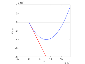
Figure 1: Comparison of the P-U energies as a function of $m$ evaluated at $\bar{n}$ in the Schrödinger and polymeric representation.

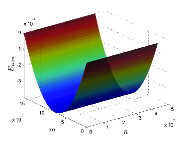
Figure 2: The polymeric P-U energy $E_{n,m}$ as a function of $n$ and $m$.

With exception of the ground state we have that the negative energy of the system increases without limit. This case may be interesting to analyze from a field point of view, since in this case the propagators turn to be suppressed by the high scale propagators . For the rigid rotator case in which $\lambda_{1}$ is large as well as $\lambda_{2}$, achieved for example taking large values of the original mass parameter $m$, one can see that the energy spectrum goes as $E_{n,m}\approx\frac{\hbar}{8}(\lambda_{1}^{2}n^{2}-\lambda_{2}^{2}m^{2})$ which can be more negative with respect to the Schrödinger representation for the same occupation numbers $(n,m)$. In this case there is no improvement for stability. Let us focus on the case $\lambda_{1}\ll 1$ and $\lambda_{2}\ll 1$ for which the total energy $E_{n,m}$ of the system can be written as

$$E_{n,m} = \frac{\hbar\omega_{1}}{2}\left((2n+1)-\frac{1}{16}(2n^{2}+2n+1)\lambda_{1}^{2}\right)$$ (47)

$$- \frac{\hbar\omega_{2}}{2}\left((2m+1)-\frac{1}{16}(2m^{2}+2m+1)\lambda_{2}^{2}\right).$$

Analogously to the Schrödinger quantization the high energy oscillator seems to lead to the instability, however we will show below that in certain regions the Hamiltonian can be defined well bounded from below. It is important to emphasize that in the absence of operators connecting the two Hilbert spaces the negative energy is not to serious and the problem of instability appears upon introducing the interactions.

Let us consider the constraints imposed on the number of normal particles $n$ that follows from the absence of any polymeric effect in quantum mechanics. From the first term in (47), it can be seen that the positive-oscillator corrections become significant or $\mathcal{O}(1)$ at the value $\bar{n}=\sqrt{h_{1}}$. For example considering the vibrational modes of a carbon monoxide molecule with mass $m=10^{-26}$ kg and frequency $\omega_{1}=10^{15}\text{s}^{-1}$, and estimating the polymer scale to be $\mu_{1}=10^{-19}$ m, we find $\bar{n}\approx 10^{7}$, see ash . In addition, in several approaches to polymer quantum mechanics a cutoff in the energy eigenvalues has been justified for the harmonic oscillator in order to implement a consistent renormalization corichi . This upper limit is key to define our effective region, since now, in contrast to what happens in the usual P-U model for higher values of the occupation number $m$ and for fixed $n=\bar{n}$ the polymeric energy is bounded from below, see Fig. 1. In the general setting where both occupation numbers $n$ and $m$ vary freely the total energy of the system is well bounded from below, avoiding possible stability problems, as shown in Fig. 2.

V Conclusions

In this work we have analyzed the stability of theories containing higher-order time derivatives within the framework of polymeric quantization. For this we have focused on the well-known Pais-Uhlenbeck model with fourth-order time derivatives in the Lagrangian. Using a canonical transformation we have cast the theory into a sum of two decoupled harmonic oscillators, one with positive energy and the other with negative energy. The negative-energy oscillator is responsible for the instabilities that arise in the presence of interactions.

We have shown that the discrete nature of the polymer Hilbert space introduces corrections in the energy spectrum of the P-U model which allows to define a region of positive defined Hamiltonian. For this we have set a cutoff from observational constraints from quantum mechanics due to the absence of any polymeric effect and further motivated by a consistent renormalization program. We have established an effective region defined by small values of the parameters $\lambda_{1}$ and $\lambda_{2}$ at which the theory has a well bounded Hamiltonian. However, for the case with large $\lambda_{1}$ and $\lambda_{2}$ , we have found that the instability shows up for very low occupation numbers with no improvement with respect to the usual Schrödinger quantization. We leave for future investigations the inclusion of interactions and the case of large $\lambda_{2}$ in the context of quantum field theory.

References

- (1) D. A. Eliezer and R. P. Woodard, Nucl. Phys. B 325, 389 (1989).
- (2) R. Gambini and J. Pullin, Phys. Rev. D 59, 124021 (1999).
- (3) J. Alfaro, H. A. Morales-Tecotl and L. F. Urrutia, Phys. Rev. Lett. 84, 2318 (2000).
- (4) J. Alfaro, H. A. Morales-Tecotl and L. F. Urrutia, Phys. Rev. D 65, 103509 (2002).
- (5) J. Alfaro, H. A. Morales-Tecotl and L. F. Urrutia, Phys. Rev. D 66, 124006 (2002).
- (6) H. Sahlmann and T. Thiemann, Class. Quant. Grav. 23, 867 (2006).
- (7) H. Sahlmann and T. Thiemann, Class. Quant. Grav. 23, 909 (2006).
- (8) V. A. Kostelecky and M. Mewes, Phys. Rev. D 80, 015020 (2009).
- (9) V. A. Kostelecky and M. Mewes, Phys. Rev. D 88, 096006 (2013).
- (10) V. A. Kostelecky and M. Mewes, Phys. Rev. D 85, 096005 (2012).
- (11) R. C. Myers and M. Pospelov, Phys. Rev. Lett. 90 (2003) 211601.
- (12) M. Schreck, Phys. Rev. D 89, 105019 (2014).
- (13) M. Schreck, Phys. Rev. D 90, 085025 (2014).
- (14) C. M. Reyes, Phys. Rev. D 82, 125036 (2010).
- (15) P. M. Crichigno and H. Vucetich, Phys. Lett. B 651, 313 (2007).
- (16) C. M. Reyes, L. F. Urrutia, J. D. Vergara, Phys. Rev. D78, 125011 (2008).
- (17) C. M. Reyes, L. F. Urrutia, J. D. Vergara, Phys. Lett. B675, 336-339 (2009).
- (18) C. M. Reyes, S. Ossandon and C. Reyes, Phys. Lett. B 746, 190 (2015).
- (19) J. R. Espinosa, B. Grinstein, D. O’Connell, M. B. Wise, Phys. Rev. D77, 085002 (2008).
- (20) B. Grinstein, D. O’Connell, M. B. Wise, Phys. Rev. D77, 025012 (2008).
- (21) T. Mariz, Phys. Rev. D 83, 045018 (2011).
- (22) T. Mariz, J. R. Nascimento and A. Y. .Petrov, Phys. Rev. D 85, 125003 (2012).
- (23) J. Leite, T. Mariz and W. Serafim, J. Phys. G 40, 075003 (2013).
- (24) R. Casana, M. M. Ferreira, Jr., R. V. Maluf and F. E. P. dos Santos, Phys. Lett. B 726, 815 (2013).
- (25) R. Casana, M. M. Ferreira, F. E. P. Dos Santos, E. O. Silva and E. Passos, arXiv:1309.3928 [hep-th].
- (26) R. Casana, M. M. Ferreira, Jr, E. O. Silva, E. Passos and F. E. P. dos Santos, Phys. Rev. D 87, no. 4, 047701 (2013).
- (27) R. Casana, M. M. Ferreira, R. V. Maluf and F. E. P. dos Santos, Phys. Rev. D 86, 125033 (2012).
- (28) F. S. Gama, M. Gomes, J. R. Nascimento, A. Y. .Petrov and A. J. da Silva, Phys. Rev. D 89, 085018 (2014).
- (29) M. A. Anacleto, F. A. Brito, O. B. Holanda, E. Passos and A. Y. .Petrov, arXiv:1405.1998 [hep-th].
- (30) I. L. Shapiro, Class. Quant. Grav. 25, 103001 (2008).
- (31) Ostrogradsky M., Mem. Acad. St. Petersbourg VI 4 (1850), 385–517.
- (32) M. S. Plyushchay, Mod. Phys. Lett. A 4, 837 (1989).
- (33) A. Pais and G. E. Uhlenbeck, Phys. Rev. 79, 145 (1950).
- (34) T. C. Cheng, P. M. Ho and M. C. Yeh, Nucl. Phys. B 625, 151 (2002).
- (35) T. C. Cheng, P. M. Ho and M. C. Yeh, Phys. Rev. D 66, 085015 (2002).
- (36) C. M. Reyes, Phys. Rev. D 80, 105008 (2009).
- (37) A. Dector, H. A. Morales-Tecotl, L. F. Urrutia and J. D. Vergara, SIGMA 5, 053 (2009).
- (38) C. M. Bender and P. D. Mannheim, Phys. Rev. Lett. 100, 110402 (2008).
- (39) C. M. Bender and P. D. Mannheim, Phys. Rev. D 78, 025022 (2008).
- (40) C. M. Bender and P. D. Mannheim, J. Phys. A 41, 304018 (2008).
- (41) S. W. Hawking and T. Hertog, Phys. Rev. D 65, 103515 (2002).
- (42) F. d. O. Salles and I. L. Shapiro, Phys. Rev. D 89, no. 8, 084054 (2014).
- (43) G. Cusin, F. d. O. Salles and I. L. Shapiro, arXiv:1503.08059 [gr-qc].
- (44) T. D. Lee and G. C. Wick, Nucl. Phys. B 9 (1969) 209.
- (45) T. D. Lee and G. C. Wick, Phys. Rev. D 2, 1033 (1970).
- (46) J. Lopez-Sarrion and C. M. Reyes, Eur. Phys. J. C 73, no. 4, 2391 (2013).
- (47) C. M. Reyes, Phys. Rev. D 87, no. 12, 125028 (2013).
- (48) M. Maniatis and C. M. Reyes, Phys. Rev. D 89, no. 5, 056009 (2014).
- (49) A. Ashtekar, S. Fairhurst and J. L. Willis, Class. Quant. Grav. 20, 1031 (2003).
- (50) M. Bojowald, Phys. Rev. Lett. 86, 5227 (2001).
- (51) G. M. Hossain, V. Husain and S. S. Seahra, Phys. Rev. D 82, 124032 (2010).
- (52) E. Flores-Gonzalez, H. A. Morales-Tecotl and J. D. Reyes, Annals Phys. 336, 394 (2013).
- (53) A. A. Garcia-Chung and H. A. Morales-Tecotl, Phys. Rev. D 89, no. 6, 065014 (2014).
- (54) J. F. Barbero G., T. Pawlowski and E. J. S. Villasenor, Phys. Rev. D 90, no. 6, 067505 (2014)
- (55) V. Husain, J. Louko and O. Winkler, Phys. Rev. D 76, 084002 (2007).
- (56) G. Kunstatter, J. Louko and J. Ziprick, Phys. Rev. A 79, 032104 (2009).
- (57) M. Bojowald, G. M. Paily and J. D. Reyes, Phys. Rev. D 90, no. 2, 025025 (2014).
- (58) G. Chacon-Acosta, E. Manrique, L. Dagdug and H. A. Morales-Tecotl, SIGMA 7, 110 (2011).
- (59) G. Chacon-Acosta and H. H. Hernandez-Hernandez, Int. J. Mod. Phys. D 24, no. 05, 1550033 (2015).
- (60) A. Corichi, T. Vukasinac and J. A. Zapata, Class. Quant. Grav. 24, 1495 (2007).
- (61) A. Corichi, T. Vukasinac and J. A. Zapata, Phys. Rev. D 76, 044016 (2007).
- (62) R. M. Wald, “Quantum field theory in curved space-time and black hole thermodynamics,” The University of Chicago Press, Chicago 60637 (1994).
- (63) L. E. Ballentine, “Quantum Mechanics,” World Scientific, (1998).
- (64) J. F. Barbero G., J. Prieto and E. J. S. Villase or, Class. Quant. Grav. 30, 165011 (2013).