Robust Connectivity Analysis for Multi-Agent Systems

Abstract.

In this report we provide a decentralized robust control approach, which guarantees that connectivity of a multi-agent network is maintained when certain bounded input terms are added to the control strategy. Our main motivation for this framework is to determine abstractions for multi-agent systems under coupled constraints which are further exploited for high level plan generation.

1. Introduction

Cooperative control of multi-agent systems constitutes a highly active area of research during the last two decades. Typical objectives are the consensus problem, which is concerned with finding a protocol that achieves convergence to a common value [9], reference tracking [1] and formation control [6]. A common feature in the approach to these problems is the design of decentralized control laws in order to achieve a global goal.

In the case of mobile robot networks with limited sensing and communication ranges, connectivity maintenance plays a fundamental role [14]. In particular, it is required to constrain the control input in such a way that the network topology remains connected during the evolution of the system. For instance, in [6] the rendezvous and formation control problems are studied while preserving connectivity, whereas in [3] swarm aggregation is achieved by means of a control scheme that guarantees both connectivity and collision avoidance.

In our approach we provide a control law for each agent comprising of a decentralized feedback component and a free input term, which ensures connectivity maintenance, for all possible free input signals up to a certain bound of magnitude. The motivation for this approach comes from distributed control and coordination of multi-agent systems with locally assigned Linear Temporal Logic (LTL) specifications. In particular, by virtue of the invariance and robust connectivity maintenance properties, it is possible to define well posed decentralized abstractions for the multi-agent system which can be exploited for motion planning. The latter problem has been studied in our recent work [2] for the single integrator dynamics case.

In this work, we design a bounded control law which results in network connectivity of the system for all future times provided that the initial relative distances of interconnected agents and the free input terms satisfy appropriate bounds. Furthermore, in the case of a spherical domain, it is shown that adding an extra repulsive vector field near the boundary of the domain can also guarantee invariance of the solutions and simultaneously maintain the robust connectivity property. The latter framework enables the construction of finite abstractions for the single integrator case.

The rest of the report is organized as follows. Section 2 introduces basic notation and preliminaries. In Section 3, results on robust connectivity maintenance are provided and explicit controllers which establish this property are designed. In Section 4, the corresponding controllers are appropriately modified, in order to additionally guarantee invariance of the solution for the case of a spherical domain. We summarize the results and discuss possible extensions in Section 5.

2. Preliminaries and Notation

2.1. Notation

We use the notation $|x|$ for the Euclidean norm of a vector $x\in\mathbb{R}^{n}$. For a matrix $A\in\mathbb{R}^{m\times n}$ we use the notation $|A|:=\max\{|Ax|:x\in\mathbb{R}^{n}\}$ for the induced Euclidean matrix norm and $A^{T}$ for its transpose. For two vectors $x,y\in\mathbb{R}^{n}(=\mathbb{R}^{n\times 1})$ we denote their inner product by $\langle x,y\rangle:=x^{T}y$. Given a subset $S$ of $\mathbb{R}^{n}$, we denote by ${\rm cl}(S)$, ${\rm int}(S)$ and $\partial S$ its closure, interior and boundary, respectively, where $\partial S:={\rm cl}(S)\setminus{\rm int}(S)$. For $R>0$, we denote by $B(R)$ the closed ball with center $0\in\mathbb{R}^{n}$ and radius $R$. Given a vector $x=(x^{1},\ldots,x^{n})\in\mathbb{R}^{n}$ we define the component operators $c_{l}(x):=x^{l}$, $l=1,\ldots,n$. Likewise, for a vector $x=(x_{1},\ldots,x_{N})\in\mathbb{R}^{Nn}$ we define the component operators $c_{l}(x):=(c_{l}(x_{1}),\ldots,c_{l}(x_{N}))\in\mathbb{R}^{N}$, $l=1,\ldots,n$.

Consider a multi-agent system with $N$ agents. For each agent $i\in\{1,\ldots,N\}:=\mathcal{N}$ we use the notation $\mathcal{N}_{i}$ for the set of its neighbors and $|\mathcal{N}_{i}|$ for its cardinality. We also consider an ordering of the agent’s neighbors which we denote by $j_{1},\ldots,j_{|\mathcal{N}_{i}|}$. $\mathcal{E}$ stands for the undirected network’s edge set and $\{i,j\}\in\mathcal{E}$ iff $j\in\mathcal{N}_{i}$. The network graph $\mathcal{G}:=(\mathcal{N},\mathcal{E})$ is connected if for each $i,j\in\mathcal{N}$ there exists a finite sequence $i_{1},\ldots,i_{l}\in\mathcal{N}$ with $i_{1}=i$, $i_{l}=j$ and $\{i_{k},i_{k+1}\}\in\mathcal{E}$, for all $k=1,\ldots,l-1$. Consider an arbitrary orientation of the network graph $\mathcal{G}$, which assigns to each edge $\{i,j\}\in\mathcal{E}$ precisely one of the ordered pairs $(i,j)$ or $(j,i)$. When selecting the pair $(i,j)$ we say that $i$ is the tail and $j$ is the head of edge $\{i,j\}$. By considering a numbering $l=1,\ldots,M$ of the graph’s edge set we define the $N\times M$ incidence matrix $D(\mathcal{G})$ corresponding to the particular orientation as follows:

$$D(\mathcal{G})_{kl}:=\left\{\begin{array}[]{ll}1,&\textup{if vertex}\;k\;\textup{is the head of edge}\;l\\ -1,&\textup{if vertex}\;k\;\textup{is the tail of edge}\;l\\ 0,&\textup{otherwise}\end{array}\right.$$

The graph Laplacian $L(\mathcal{G})$ is the $N\times N$ positive semidefinite symmetric matrix $L(\mathcal{G}):=D(\mathcal{G})\times D(\mathcal{G})^{T}$. If we denote by $\mathbb{1}$ the vector $(1,\ldots,1)\in\mathbb{R}^{N}$, then $L(\mathcal{G})\mathbb{1}=D(\mathcal{G})^{T}\mathbb{1}=0$. Let $0=\lambda_{1}(\mathcal{G})\leq\lambda_{2}(\mathcal{G})\leq\cdots\leq\lambda_{N}(\mathcal{G})$ be the ordered eigenvalues of $L(\mathcal{G})$. Then each corresponding set of eigenvectors is orthogonal and $\lambda_{2}(\mathcal{G})>0$ iff $\mathcal{G}$ is connected.

2.2. Problem Statement

We focus on single integrator multi-agent systems with dynamics

$$\dot{x}_{i}=u_{i},x_{i}\in\mathbb{R}^{n},i=1,\ldots,N$$ (2.1)

We aim at designing decentralized control laws of the form

$$u_{i}:=k_{i}(x_{i},x_{j_{1}},\ldots,x_{j_{|\mathcal{N}_{i}|}})+v_{i}$$ (2.2)

which ensure that appropriate apriori bounds on the initial relative distances of interconnected agents guarantee network connectivity for all future times, for all free inputs $v_{i}$ bounded by certain constant. In particular, we assume that the network graph is connected as long as the maximum distance between two interconnected agents does not exceed a given positive constant $R$. In addition, we make the following connectivity hypothesis for the initial states of the agents.

(ICH) We assume that the agents’ communication graph is initially connected and that

$$\max\{|x_{i}(0)-x_{j}(0)|:\{i,j\}\in\mathcal{E}\}\leq\tilde{R}\;\textup{for certain constant}\;\tilde{R}\in(0,R)$$ (2.3)

2.3. Potential Functions

We proceed by defining certain mappings which we exploit in order to design the control law (2.2) and prove that network connectivity is maintained. Let $r:\mathbb{R}_{\geq 0}\to\mathbb{R}_{\geq 0}$ be a continuous function satisfying the following property.

(P) $r(\cdot)$ is increasing and $r(0)>0$.

Also, consider the integral

$$P(\rho)=\int_{0}^{\rho}r(s)sds,\rho\in\mathbb{R}_{\geq 0}$$ (2.4)

For each pair $(i,j)\in\mathcal{N}\times\mathcal{N}$ with $\{i,j\}\in\mathcal{E}$ we define the potential function $V_{ij}:\mathbb{R}^{Nn}\to\mathbb{R}_{\geq 0}$ as

$$V_{ij}(x)=P(|x_{i}-x_{j}|),\forall x=(x_{1},\ldots,x_{N})\in\mathbb{R}^{Nn}$$ (2.5)

Notice that $V_{ij}(\cdot)=V_{ji}(\cdot)$. Furthermore, it can be shown that $V_{ij}(\cdot)$ is continuously differentiable and that

$$\frac{\partial}{\partial x_{i}}V_{ij}(x)=r(|x_{i}-x_{j}|)(x_{i}-x_{j})^{T}$$ (2.6)

where $\frac{\partial}{\partial x_{i}}$ stands for the derivative with respect to the $x_{i}$-coordinates.

Remark 2.1.

Notice that we are only interested in the values of the mappings $r(\cdot)$ and $P(\cdot)$ in the interval $[0,R]$, which stands for the maximum distance that two interconnected agents may achieve before losing connectivity. Yet, defining them on the whole positive line provides us certain technical flexibilities for the analysis employed in the proof of connectivity maintenance.

3. Connectivity Analysis

In the following proposition we provide a control law (2.2) and an upper bound on the magnitude of the input terms $v_{i}(\cdot)$ which guarantee connectivity of the multi-agent network.

Proposition 3.1.

For the multi-agent system (2.1), assume that (ICH) is fulfilled and define the control law

$$u_{i}=-\sum_{j\in\mathcal{N}_{i}}r(|x_{i}-x_{j}|)(x_{i}-x_{j})+v_{i}$$ (3.1)

for certain continuous $r(\cdot)$ satisfying Property (P). Also, consider a constant $\delta>0$ and define

$$K:=\frac{2\sqrt{N(N-1)}|D(\mathcal{G})^{T}|}{\lambda_{2}(\mathcal{G})^{2}}$$ (3.2)

where $D(\mathcal{G})$ is the incidence matrix of the systems’ graph and $\lambda_{2}(\mathcal{G})$ the second eigenvalue of the graph Laplacian. We assume that the positive constant $\delta$, the maximum initial distance $\tilde{R}$ and the function $r(\cdot)$ satisfy the restrictions

$$\delta\leq\frac{1}{K}r(0)^{2}\frac{s}{r(s)},s\geq\tilde{R}$$ (3.3)

with $K$ as given in (3.2) and

$$MP(\tilde{R})\leq P(R)$$ (3.4)

where $P(\cdot)$ is given in (2.4), and $M=|\mathcal{E}|$ is the cardinality of the system’s graph edge set. Then, the system remains connected for all positive times, provided that the input terms $v_{i}(\cdot)$, $i=1,\ldots,N$ satisfy

$$|v_{i}(t)|\leq\delta,\forall t\geq 0$$ (3.5)

Proof.

For the proof we follow parts of the analysis in [6] (see also [8, Section 7.2]). Consider the energy function

$$V:=\frac{1}{2}\sum_{i=1}^{N}\sum_{j\in\mathcal{N}_{i}}V_{ij}$$ (3.6)

where the mappings $V_{ij}$, $\{i,j\}\in\mathcal{E}$ are given in (2.5). Then it follows from (2.6) that

$$\frac{\partial}{\partial x_{i}}V(x)=\sum_{j\in\mathcal{N}_{i}}r(|x_{i}-x_{j}|)(x_{i}-x_{j})^{T}$$ (3.7)

Also, in accordance with [8, Section 7.2] we have for $l=1,\ldots,n$ that

$$c_{l}\left(\sum_{j\in\mathcal{N}_{i}}r(|x_{i}-x_{j}|)(x_{i}-x_{j})\right)=L_{w}(x)c_{l}(x)$$ (3.8)

The weighted Laplacian matrix $L_{w}(x)$ is given as

$$L_{w}(x)=D(\mathcal{G})W(x)D(\mathcal{G})^{T}$$ (3.9)

where $D(\mathcal{G})$ is the incidence matrix of the communication graph (see Notation) and

$$W(x):={\rm diag}\{w_{1}(x),\ldots,w_{M}(x)\}:={\rm diag}\{r(|x_{i}-x_{j}|),\{i,j\}\in\mathcal{E}\}$$ (3.10)

(recall that $M=|\mathcal{E}|$). Then, by evaluating the time derivative of $V$ along the trajectories of (2.1)-(3.1) and taking into account (3.6), (3.7) and (3.8) we get

$$\dot{V} =-\sum_{l=1}^{n}c_{l}\left(\frac{\partial}{\partial x}V(x)\right)c_{l}(\dot{x})$$

$$=-\sum_{l=1}^{n}c_{l}(x)^{T}L_{w}(x)(L_{w}(x)c_{l}(x)-c_{l}(v))$$

$$=-\sum_{l=1}^{n}c_{l}(x)^{T}L_{w}(x)^{2}c_{l}(x)+\sum_{l=1}^{n}c_{l}(x)^{T}L_{w}(x)c_{l}(v)$$

$$\leq-\sum_{l=1}^{n}c_{l}(x)^{T}L_{w}(x)^{2}c_{l}(x)+\left|\sum_{l=1}^{n}c_{l}(x)^{T}L_{w}(x)c_{l}(v)\right|$$ (3.11)

We want to provide appropriate bounds for the right hand side of (3.11) which can guarantee that the sign of $\dot{V}$ is negative whenever the maximum distance between two agents exceeds the bound $\tilde{R}$ on the maximum initial distance as given in (2.3). First, we provide certain useful inequalities between the eigenvalues of the weighted Laplacian $L_{w}(x)$ and the Laplacian matrix of the graph $L(\mathcal{G})$. Notice, that due to (3.10), for each $i=1,\ldots,M$ we have $w_{i}(x)=r(|x_{k}-x_{\ell}|)$ for certain $\{k,\ell\}\in\mathcal{E}$ and hence, by virtue of Property (P), it holds

$$0<r(0)\leq w_{i}(x)\leq\max_{\{k,\ell\}\in\mathcal{E}}r(|x_{k}-x_{\ell}|)$$ (3.12)

From (3.12), it follows that $L_{w}(x)$ has precisely the same properties with those provided for $L(\mathcal{G})$ in the Notation subsection. Furthermore, it holds

$$\lambda_{2}(x)\geq\lambda_{2}(\mathcal{G})r(0)$$ (3.13)

where $0=\lambda_{1}(x)<\lambda_{2}(x)\leq\cdots\leq\lambda_{N}(x)$ and $0=\lambda_{1}(\mathcal{G})<\lambda_{2}(\mathcal{G})\leq\cdots\leq\lambda_{N}(\mathcal{G})$ are the eigenvalues of $L_{w}(x)$ and the Laplacian matrix of the graph $L(\mathcal{G})$, respectively. Indeed, in order to show (3.13), notice that

$$L_{w}(x) =D(\mathcal{G}){\rm diag}\{w_{1}(x),\ldots,w_{M}(x)\}D(\mathcal{G})^{T}$$

$$=D(\mathcal{G}){\rm diag}\{r(0),\ldots,r(0)\}D(\mathcal{G})^{T}$$

$$+D(\mathcal{G}){\rm diag}\{w_{1}(x)-r(0),\ldots,w_{M}(x)-r(0)\}D(\mathcal{G})^{T}=r(0)L(\mathcal{G})+B$$

where (3.12) implies that $B:=D(\mathcal{G}){\rm diag}\{w_{1}(x)-r(0),\ldots,w_{M}(x)-r(0)\}D(\mathcal{G})^{T}$ is positive semidefinite. Hence, it holds $L_{w}(x)\succeq r(0)L(\mathcal{G})$, with $\succeq$ being the partial order on the set of symmetric $N\times N$ matrices and thus, we deduce from Corollary 7.7.4(c) in [4, page 495] that (3.13) is fulfilled.

In the sequel we introduce some additional notation. Let $H$ be the subspace

$$H:=\{x\in\mathbb{R}^{Nn}:x_{1}=x_{2}=\cdots=x_{N}\}$$

For a vector $x\in\mathbb{R}^{Nn}$ we denote by $\bar{x}$ its projection to the subspace $H$, and $x^{\perp}$ its orthogonal complement with respect to that subspace, namely $x^{\perp}:=x-\bar{x}$. By taking into account that for all $y\in H$ we have $D(\mathcal{G})^{T}c_{l}(y)=0$ and hence, due to (3.9), that $c_{l}(y)\in\ker(L_{w}(x))$, it follows that for every vector $x\in\mathbb{R}^{Nn}$ with $x=\bar{x}+x^{\perp}$ it holds

$$L_{w}(x)c_{l}(\bar{x})=0\Rightarrow L_{w}(x)c_{l}(x)=L_{w}(x)c_{l}(\bar{x}+x^{\perp})=L_{w}(x)c_{l}(x^{\perp})$$ (3.14)

We also denote by $\Delta x\in\mathbb{R}^{Mn}$ the stack column vector of the vectors $x_{i}-x_{j},\{i,j\}\in\mathcal{E}$ with the edges ordered as in the case of the incidence matrix. It is thus straightforward to check that for all $x\in\mathbb{R}^{Nn}$

$$D(\mathcal{G})^{T}x=\Delta x$$ (3.15)

and furthermore, due to (3.10) and (3.12), that

$$|W(x)|\leq r(|\Delta x|_{\infty})$$ (3.16)

where

$$|\Delta x|_{\infty}:=\max\{|\Delta x_{i}|,i=1,\ldots,M\}$$ (3.17)

Before proceeding we state the following elementary facts, whose proofs can be found in the Appendix. In particular, for the vectors $x=(x_{1},\ldots,x_{N}),y=(y_{1},\ldots,y_{N})\in\mathbb{R}^{Nn}$ the following properties hold.

Fact I.

$$|L_{w}(x)c_{l}(x^{\perp})|\geq\lambda_{2}(x)|c_{l}(x^{\perp})|,\forall l=1,\ldots,n$$ (3.18)

Fact II.

$$\sum_{l=1}^{n}|c_{l}(x)||c_{l}(y)|\leq|x||y|$$ (3.19)

Fact III.

$$|x^{\perp}|\geq\frac{1}{\sqrt{2(N-1)}}|\Delta x|$$ (3.20)

Fact IV.

$$\sqrt{2}|x^{\perp}|\geq|\Delta x|_{\infty}$$ (3.21)

We are now in position to bound the derivative of the energy function $V$ and exploit the result in order to prove the desired connectivity maintenance property. We break the subsequent proof in two main steps.

Step 1: Bound estimation for the rhs of (3.11).

Bound for the first term in (3.11). By taking into account (3.14), it follows that

$$\sum_{l=1}^{n}c_{l}(x)^{T}L_{w}(x)^{2}c_{l}(x)=\sum_{l=1}^{n}\left|L_{w}(x)c_{l}(x)\right|^{2}=\sum_{l=1}^{n}\left|L_{w}(x)c_{l}(x^{\perp})\right|^{2}$$ (3.22)

and by exploiting Fact I and (3.13), we get

$$\sum_{l=1}^{n}\left|L_{w}(x)c_{l}(x^{\perp})\right|^{2} \geq\sum_{l=1}^{n}\lambda_{2}(x)^{2}|c_{l}(x^{\perp})|^{2}\geq\sum_{l=1}^{n}[\lambda_{2}(\mathcal{G})r(0)]^{2}|c_{l}(x^{\perp})|^{2}$$

$$=[\lambda_{2}(\mathcal{G})r(0)]^{2}\sum_{l=1}^{n}\left|c_{l}(x^{\perp})\right|^{2}=[\lambda_{2}(\mathcal{G})r(0)]^{2}|x^{\perp}|^{2}$$ (3.23)

Thus, it follows from (3.22) and (3.23) that

$$\sum_{l=1}^{n}c_{l}(x)^{T}L_{w}(x)^{2}c_{l}(x)\geq[\lambda_{2}(\mathcal{G})r(0)]^{2}|x^{\perp}|^{2}$$ (3.24)

Bound for the second term in (3.11). For this term, we have from (3.9) and (3.15) that

$$\left|\sum_{l=1}^{n}c_{l}(x)^{T}L_{w}(x)c_{l}(v)\right| \leq\sum_{l=1}^{n}|c_{l}(x)^{T}L_{w}(x)c_{l}(v)|$$

$$=\sum_{l=1}^{n}|c_{l}(x)^{T}D(\mathcal{G})W(x)D(\mathcal{G})^{T}c_{l}(v)|$$

$$=\sum_{l=1}^{n}|c_{l}(\Delta x)^{T}W(x)D(\mathcal{G})^{T}c_{l}(v)|$$

$$\leq\sum_{l=1}^{n}|c_{l}(\Delta x)||W(x)||D(\mathcal{G})^{T}||c_{l}(v)|$$ (3.25)

By taking into account (3.16), we obtain

$$\sum_{l=1}^{n}|c_{l}(\Delta x)||W(x)||D(\mathcal{G})^{T}||c_{l}(v)|\leq\sum_{l=1}^{n}|c_{l}(\Delta x)|r(|\Delta x|_{\infty})|D(\mathcal{G})^{T}||c_{l}(v)|$$ (3.26)

Also, by exploiting Fact II, we get that

$$\sum_{l=1}^{n}|c_{l}(\Delta x)|r(|\Delta x|_{\infty}) |D(\mathcal{G})^{T}||c_{l}(v)|$$

$$= r(|\Delta x|_{\infty})|D(\mathcal{G})^{T}|\sum_{l=1}^{n}|c_{l}(\Delta x)||c_{l}(v)|$$

$$\leq r(|\Delta x|_{\infty})|D(\mathcal{G})^{T}||\Delta x||c_{l}(v)|$$

$$\leq r(|\Delta x|_{\infty})|D(\mathcal{G})^{T}||\Delta x|\sqrt{N}|v|_{\infty}$$ (3.27)

where

$$|v|_{\infty}:=\max\{|v_{i}|,i=1,\ldots,N\}$$

Hence, it follows from (3)-(3) that

$$\left|\sum_{l=1}^{n}c_{l}(x)^{T}L_{w}(x)c_{l}(v)\right|\leq\sqrt{N}|D(\mathcal{G})^{T}||\Delta x|r(|\Delta x|_{\infty})|v|_{\infty}$$ (3.28)

Thus, we get from (3.11), (3.24) and (3.28) that

$$\dot{V}\leq-[\lambda_{2}(\mathcal{G})r(0)]^{2}|x^{\perp}|^{2}+\sqrt{N}|D(\mathcal{G})^{T}||\Delta x|r(|\Delta x|_{\infty})|v|_{\infty}$$

and by exploiting Facts III and IV, that

$$\dot{V} \leq-[\lambda_{2}(\mathcal{G})r(0)]^{2}\frac{1}{\sqrt{2(N-1)}}|\Delta x|\frac{1}{\sqrt{2}}|\Delta x|_{\infty}+\sqrt{N}|D(\mathcal{G})^{T}||\Delta x|r(|\Delta x|_{\infty})|v|_{\infty}$$

$$=|\Delta x|\left(-\frac{1}{2\sqrt{N-1}}[\lambda_{2}(\mathcal{G})r(0)]^{2}|\Delta x|_{\infty}+\sqrt{N}|D(\mathcal{G})^{T}|r(|\Delta x|_{\infty})|v|_{\infty}\right)$$

By using the notation $|\Delta x|_{\infty}:=s$, in order to guarantee that the above rhs is negative for $s\geq\tilde{R}$, it should hold

$$-\frac{\lambda_{2}(\mathcal{G})^{2}}{2\sqrt{(N-1)}}r(0)^{2}s+\sqrt{N}|D(\mathcal{G})^{T}|r(s)|v|_{\infty}\leq 0,\forall s\geq\tilde{R}\iff$$

$$\frac{2\sqrt{N(N-1)}|D(\mathcal{G})^{T}|}{\lambda_{2}(\mathcal{G})^{2}}|v|_{\infty}\leq r(0)^{2}\frac{s}{r(s)},\forall s\geq\tilde{R}$$

or equivalently

$$|v|_{\infty}\leq\frac{1}{K}r(0)^{2}\frac{s}{r(s)},\forall s\geq\tilde{R}$$ (3.29)

with $K$ as given in (3.2). Hence, we have shown that for $v$ satisfying (3.29) the following implication holds

$$|\Delta x|_{\infty}\geq\tilde{R}\Rightarrow\dot{V}\leq 0$$ (3.30)

Step 2: Proof of connectivity.

By assuming that conditions (3.5), (3.3) and (3.4) in the statement of the proposition are fulfilled and recalling that according to (ICH) (2.3) holds, we can show that the system will remain connected for all future times. Indeed, let $x(\cdot)$ be the solution of the closed loop system (2.1)-(3.1) with initial condition satisfying (2.3), defined on the maximal right interval $[0,T_{\max})$. We claim that the system remains connected on $[0,T_{\max})$, namely, that $\max\{|x_{i}(t)-x_{j}(t)|:\{i,j\}\in\mathcal{E}\}\leq R$ for all $t\in[0,T_{\max})$, which by boundedness of the dynamics on the set $\mathcal{F}:=\{x\in\mathbb{R}^{Nn}:|x_{i}-x_{j}|\leq R,\forall\{i,j\}\in\mathcal{E}\}$ implies that $T_{\max}=\infty$. In order to prove the last assertion, assume on the contrary that $T_{\max}<\infty$. Then, by taking into account that $x(t)$ remains in $\mathcal{F}$ for all $t\in[0,T_{\max})$ and that the dynamics are bounded on $\mathcal{F}$, it follows that $x(t)$ remains in a compact subset of $\mathbb{R}^{Nn}$ for all $t\in[0,T_{\max})$ and hence, that it can be extended, contradicting maximality of $[0,T_{\max})$. We proceed with the proof of connectivity. First, notice that

$$V(x(0))\leq\frac{1}{2}P(R)$$ (3.31)

Indeed, by exploiting (2.3) and (3.4) we get that

$$V(x(0)) =\frac{1}{2}\sum_{i=1}^{N}\sum_{j\in\mathcal{N}_{i}}P(|x_{i}(0)-x_{j}(0)|)$$

$$\leq\frac{1}{2}\sum_{i=1}^{N}\sum_{j\in\mathcal{N}_{i}}P(\tilde{R})=\frac{M}{2}P(\tilde{R})\leq\frac{1}{2}P(R)$$ (3.32)

In order to prove our claim, it suffices to show that

$$V(x(t))\leq\frac{1}{2}P(R),\forall t\in[0,T_{\max})$$ (3.33)

because if $|x_{i}(t)-x_{j}(t)|>R$ for certain $t\in[0,T_{\max})$ and $\{i,j\}\in\mathcal{E}$, then $V(x(t))\geq\frac{1}{2}P(|x_{i}(t)-x_{j}(t)|)>\frac{1}{2}P(R)$. We prove (3.33) by contradiction. Indeed, suppose on the contrary that there exists $T\in(0,T_{\max})$ (due to (3.31)) such that

$$V(x(T))>\frac{1}{2}P(R)$$ (3.34)

and define

$$\tau:=\min\{t\in[0,T]:V(x(\bar{t}))>\tfrac{1}{2}P(R),\forall\bar{t}\in(t,T]\}$$ (3.35)

which due to (3.34) and continuity of $V(x(\cdot))$ is well defined. Then it follows from (3.31) and (3.35) that

$$V(x(\tau))=\frac{1}{2}P(R),V(x(t))>\frac{1}{2}P(R),\forall t\in(\tau,T]$$ (3.36)

hence, there exists $\bar{\tau}\in(\tau,T)$ such that

$$\dot{V}(x(\bar{\tau}))=\frac{V(x(T))-V(x(\tau))}{T-\tau}>0$$ (3.37)

On the other hand, due to (3.36), it holds

$$V(x(\bar{\tau}))>\frac{1}{2}P(R)$$ (3.38)

which implies that there exists $\{i,j\}\in\mathcal{E}$ with

$$|x_{i}(\bar{\tau})-x_{j}(\bar{\tau})|>\tilde{R}$$ (3.39)

Indeed, if (3.39) does not hold, then we can show as in (3.32) that $V(x(\bar{\tau}))\leq\frac{1}{2}P(R)$ which contradicts (3.38). Notice that by virtue of (3.5) and (3.3), (3.29) is fulfilled. Hence, we get from (3.39) that $|\Delta x(\bar{\tau})|_{\infty}>\tilde{R}$ and thus from (3.30) it follows that $\dot{V}(x(\bar{\tau}))\leq 0$, which contradicts (3.37). We conclude that (3.33) holds and the proof is complete. ∎

In the following corollary, we apply the result of Proposition 3.1 in order to provide two explicit feedback laws of the form (3.1), a linear and a nonlinear one and compare their performance in the subsequent remark.

Corollary 3.2.

For the multi agent system (2.1), assume that (ICH) is fulfilled and consider the control law (2.2) as given by (3.1). By imposing the additional requirement $r(0)=r(\tilde{R})=1$ and defining

$$\delta:=\frac{\tilde{R}}{K}$$ (3.40)

with $\tilde{R}$ and $K$ as given in (2.3) and (3.2), respectively, the system remains connected for all positive times, provided that the function $r(\cdot)$ and the constant $\tilde{R}$ are selected as in the following two cases (L) and (NL) (providing a linear and a nonlinear feedback, respectively).

Case (L). We select

$$r(s):=1,s\geq 0$$ (3.41)

and

$$\tilde{R}\leq\frac{1}{\sqrt{M}}R$$ (3.42)

where $M$ is the cardinality of the system’s graph edge set.

Case (NL). We select

$$r(s):=\left\{\begin{array}[]{ll}1,&s\in[0,\tilde{R}]\\ \frac{s}{\tilde{R}},&s\in(\tilde{R},R]\\ \frac{R}{\tilde{R}},&s\in(R,\infty)\end{array}\right.$$ (3.43)

and

$$\tilde{R}\leq\left(\frac{2}{3M-1}\right)^{\frac{1}{3}}R$$ (3.44)

Proof.

For the proof we apply the result of Proposition (3.1). In particular, it suffices to show that for both cases (L) and (NL) the selection of the function $r(\cdot)$ and the initial maximum distance $\tilde{R}$ satisfy (3.3) and (3.4), with $\delta$ as given by (3.40).

Case (L). Indeed, it follows from (3.40) and (3.41) that

$$\delta=\frac{\tilde{R}}{K}=\frac{1}{K}\frac{\tilde{R}}{r(s)}r(0)^{2}\leq\frac{1}{K}\frac{s}{r(s)}r(0)^{2},\forall s\geq\tilde{R}$$

hence, (3.3) is fulfilled. Furthermore, it follows from (3.41) and (2.4) that

$$MP(\tilde{R})\leq P(R) \iff M\int_{0}^{\tilde{R}}r(s)sds\leq\int_{0}^{R}r(s)sds$$

$$\iff M\int_{0}^{\tilde{R}}sds\leq\int_{\tilde{R}}^{R}sds\iff M\frac{\tilde{R}^{2}}{2}\leq\frac{R^{2}}{2}\iff\tilde{R}\leq\frac{1}{\sqrt{M}}R$$

Case (NL). Also in this case, it follows from (3.40) and (3.43) that

$$\delta=\frac{\tilde{R}}{K}=\frac{\tilde{R}}{K}\frac{s}{s}r(0)^{2}\leq\frac{1}{K}\frac{s}{\frac{s}{\tilde{R}}}r(0)^{2}=\frac{1}{K}\frac{s}{r(s)}r(0)^{2},\forall s\in(\tilde{R},R]$$

and that

$$\delta =\frac{\tilde{R}}{K}\leq\frac{\tilde{R}}{K}\frac{s}{R}r(0)^{2}$$

$$=\frac{1}{K}\frac{s}{\frac{s}{\tilde{R}}}r(0)^{2}\leq\frac{1}{K}\frac{s}{\frac{R}{\tilde{R}}}r(0)^{2}=\frac{1}{K}\frac{s}{r(s)}r(0)^{2},\forall s\geq R$$

hence, (3.3) is again fulfilled. In addition, it follows from (3.43) and (2.4) that

$$MP(\tilde{R})\leq P(R) \iff M\int_{0}^{\tilde{R}}r(s)sds\leq\int_{0}^{R}r(s)sds$$

$$\iff M\int_{0}^{\tilde{R}}r(s)sds\leq\int_{0}^{\tilde{R}}r(s)sds+\int_{\tilde{R}}^{R}r(s)sds$$

$$\iff(M-1)\int_{0}^{\tilde{R}}sds\leq\frac{1}{\tilde{R}}\int_{\tilde{R}}^{R}s^{2}ds\iff(M-1)\frac{\tilde{R}^{2}}{2}\leq\frac{1}{\tilde{R}}\left.\frac{1}{3}s^{3}\right|_{\tilde{R}}^{R}$$

$$\iff\frac{M-1}{2}\tilde{R}^{3}\leq\frac{1}{3}R^{3}-\frac{1}{3}\tilde{R}^{3}\iff\frac{3M-3}{6}\tilde{R}^{3}+\frac{2}{6}\tilde{R}^{3}\leq\frac{1}{3}R^{3}$$

$$\iff\frac{3M-1}{2}\tilde{R}^{3}\leq R^{3}\iff\tilde{R}\leq\left(\frac{2}{3M-1}\right)^{\frac{1}{3}}R$$

∎

Remark 3.3.

At this point we derive the advantage of using the nonlinear controller over the linear one by comparing the ratio of the maximal initial relative distance that maintains connectivity for these two cases. In both cases we have the same bound on the free input terms and the same feedback law up to some distance between neighboring agents, which allows us to compare their performance under the criterion of maximizing the largest initial distance between two interconnected agents. In particular, this ratio, which depends on the number of edges in the systems’ graph, is given by

$$Rat(M):=\frac{\frac{1}{\sqrt{M}}}{\left(\frac{2}{3M-1}\right)^{\frac{1}{3}}}$$ (3.45)

It is evident from the plot of $Rat(M)$ in Figure 1 that it is a decreasing function of $M$ with values less than 1 for $M\geq 1$. The latter property follows quite intuitively if we take a look at Figure 2. Indeed, as sown in the proof of Proposition (3.1), both the maximal initial distance $\tilde{R}_{L}$ for the linear and $\tilde{R}_{NL}$ for the nonlinear case are expressed by virtue of (3.4) as the solutions of the equation $\frac{P(\tilde{R})}{P(R)-P(\tilde{R})}=\frac{1}{M-1}$. In Figure 2, both the quotient of the area inside the orange frame over the area in the red frame and the quotient of the violet area over the blue area are the same and equal to $\frac{P(\tilde{R})}{P(R)-P(\tilde{R})}=\frac{1}{M-1}$, with $P(\cdot)$ as defined for both the cases (L) and (NL) through (2.4), (3.41) and (3.43). It is thus straightforward that the quotient of $\tilde{R}_{L}$ over $\tilde{R}_{NL}$, namely $Rat(M)$ should be less than 1. Yet, we also provide a formal proof of this argument by studying the monotonicity of $Rat(\cdot)$.

For convenience we consider the 6-th power of $Rat(M)$, namely the function

$$Rat^{6}(M):=\left[\frac{\frac{1}{\sqrt{M}}}{\left(\frac{2}{3M-1}\right)^{\frac{1}{3}}}\right]^{6}=\frac{(3M-1)^{2}}{{2^{3}M^{3}}}$$

Hence, by evaluating the derivative of $Rat^{6}(M)$ we obtain

$$\frac{d}{dM}Rat^{6}(M) =\frac{d}{dM}\frac{(3M-1)^{2}}{{2^{3}M^{3}}}=\frac{2(3M-1)3\cdot 2^{3}M^{3}-(3M-1)^{2}2^{3}3M^{2}}{2^{6}M{6}}$$

$$=\frac{3\cdot 2^{3}M^{2}(3M-1)[2M-(3M-1)]}{2^{6}M^{6}}=\frac{3}{2^{3}}\cdot\frac{3M-1}{M^{4}}(1-M)<0,\;{\rm for}\;M>1$$

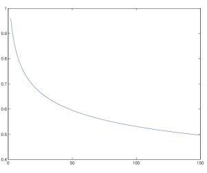
Figure 1. This figure shows the ratio $\frac{1}{\sqrt{M}}\;/\;\left(\frac{2}{3M-1}\right)^{\frac{1}{3}}$ for the number of edges ranging from 2 to 150

Figure 2. $\tilde{R}_{L}$ and $\tilde{R}_{NL}$ and norms of the respective feedback control laws for $M=12$

4. Invariance Analysis

In what follows, we assume that the agents’ initial states belong to a given domain $D\subset\mathbb{R}^{n}$. In order to simplify the subsequent analysis, we assume that $D={\rm int}(B(\mathfrak{R}))$, namely the interior of the ball with center $0\in\mathbb{R}^{n}$ and radius $\mathfrak{R}>0$. We aim at designing an appropriate modification of the feedback law (3.1) which guarantees that the trajectories of the agents remain in $D$ for all future times.

For each $\varepsilon\in(0,\mathfrak{R})$, let $N_{\varepsilon}$ be the region with distance $\varepsilon$ from the boundary of $\partial D$ towards the interior of $D$, namely

$$N_{\varepsilon}:=\{x\in\mathbb{R}^{n}:R-\varepsilon\leq|x|<R\}$$ (4.1)

and

$$D_{\varepsilon}:=D\setminus N_{\varepsilon}$$ (4.2)

We proceed by defining a repulsive from the boundary of $D$ vector field, which when added to the dynamics of each agent in (3.1), will ensure the desired invariance of the closed loop system and simultaneously guarantee the same robust connectivity result established above. Let $h:[0,1]\to[0,1]$ be a Lipschitz continuous function that satisfies

$$h(0)=0;\;h(1)=1;\;h(\cdot)\;\textup{strictly increasing}$$ (4.3)

We define the vector field $g:D\to\mathbb{R}^{n}$ as

$$g(x):=\left\{\begin{array}[]{ll}-c\delta h\left(\frac{\varepsilon+|x|-R}{\varepsilon}\right)\frac{x}{|x|},&{\rm if}\;x\in N_{\varepsilon}\\ 0,&{\rm if}\;x\in D_{\varepsilon}\end{array}\right.$$ (4.4)

with $h(\cdot)$ as given above and appropriate positive constants $c$, $\delta$ which serve as design parameters. Then, it follows from (4.3), (4.4) and the Lipschitz property for $h(\cdot)$ that the vector field $g(\cdot)$ is Lipschitz continuous on $D$.

Having defined the mappings for the extra term in the dynamics of the modified controller which will guarantee the desired invariance property, we now state our main result.

Proposition 4.1.

For the multi-agent system (2.1), assume that $D={\rm int}(B(\mathfrak{R}))$, for certain $\mathfrak{R}>0$ and that (ICH) is fulfilled. Furthermore, let $\varepsilon\in(0,\mathfrak{R})$, $N_{\varepsilon}$ and $D_{\varepsilon}$ as defined by (4.1) and (4.2), respectively and assume that the initial states of all agents lie in $D_{\varepsilon}$. Then, there exists a control law (2.2) (with free inputs $v_{i}$) which guarantees both connectivity and invariance of $D$ for the solution of the system for all future times and is defined as

$$u_{i}=g(x_{i})-\sum_{j\in\mathcal{N}_{i}}r(|x_{i}-x_{j}|)(x_{i}-x_{j})+v_{i}$$ (4.5)

with $g(\cdot)$ given in (4.4) and certain $r(\cdot)$ satisfying Property (P). We choose the same positive constant $\delta$ in both (3.5) and (4.4) and select the constant $c$ in (4.4) greater that 1. Then the connectivity-invariance result is valid provided that the parameters $\delta$, $\tilde{R}$ and the function $r(\cdot)$ satisfy the restrictions (3.3), (3.4) and the input terms $v_{i}(\cdot)$, $i=1,\ldots,N$ satisfy (3.5).

Proof.

We break the proof in two steps. In the first step, we show that as long as the invariance assumption is satisfied, namely, the solution of the closed loop system (2.1)-(4.5) is defined and remains in $D$, network connectivity is maintained. In the second step, we show that for all times where the solution is defined, it remains inside a compact subset of $D$, which implies that the solution is defined and remains in $D$ for all future times, thus providing the desired invariance property.

Step 1: Proof of network connectivity.

The proof of this step is based on an appropriate modification of the corresponding proof of Proposition 3.1. In particular, we exploit the energy function $V$ as given by (3.6) and show that when $|\Delta x|_{\infty}\geq\tilde{R}$, namely, when the maximum distance between two agents exceeds $\tilde{R}$ then its derivative along the solutions of the closed loop system is negative. Thus by using the same arguments with those in proof of Proposition 3.1 we can deduce that the system remains connected. Indeed, by evaluating the derivative of $V$ along the solutions of (2.1)-(4.5) we obtain

$$\dot{V} =\sum_{i=1}^{N}\frac{\partial}{\partial x_{i}}V(x)\dot{x}_{i}$$

$$=\sum_{i=1}^{N}\frac{\partial}{\partial x_{i}}V(x)g(x_{i})-\sum_{l=1}^{n}c_{l}(x)^{T}L_{w}(x)^{2}c_{l}(x)+\sum_{l=1}^{n}c_{l}(x)^{T}L_{w}(x)c_{l}(v)$$

$$\leq\sum_{i=1}^{N}\frac{\partial}{\partial x_{i}}V(x)g(x_{i})-\sum_{l=1}^{n}c_{l}(x)^{T}L_{w}(x)^{2}c_{l}(x)+\left|\sum_{l=1}^{n}c_{l}(x)^{T}L_{w}(x)c_{l}(v)\right|$$ (4.6)

By taking into account (3.11) and using precisely the same arguments with those in proof of Steps 1 and 2 of Proposition 3.1 it suffices to show that the first term of inequality (4.6), which by virtue of (3.7) is equal to

$$\sum_{i=1}^{N}\frac{\partial}{\partial x_{i}}V(x)g(x_{i})=\sum_{i=1}^{N}\sum_{j\in\mathcal{N}_{i}}r(|x_{i}-x_{j}|)\langle(x_{i}-x_{j}),g(x_{i})\rangle$$

is nonpositive for all $x\in D$. Given the partition $D_{\varepsilon}$, $N_{\varepsilon}$ of $D$, we consider for each agent $i\in\mathcal{N}$ the partition $\mathcal{N}_{i}^{D_{\varepsilon}}$, $\mathcal{N}_{i}^{N_{\varepsilon}}$ of its neighbors’ set, corresponding to its neighbors that belong to $D_{\varepsilon}$ and $N_{\varepsilon}$, respectively. Also, we denote by $\mathcal{E}^{N_{\varepsilon}}$ the set of edges $\{i,j\}$ with both $x_{i},x_{j}\in N_{\varepsilon}$. Then, by taking into account that due to (4.4), $g(x_{i})=0$ for $x_{i}\in D_{\varepsilon}$, it follows that

$$\sum_{i=1}^{N}\sum_{j\in\mathcal{N}_{i}}r(|x_{i}-x_{j}|)\langle(x_{i}-x_{j}),g(x_{i})\rangle$$

$$= \sum_{\{i\in\mathcal{N}:x_{i}\in N_{\varepsilon}\}}\sum_{j\in\mathcal{N}_{i}}r(|x_{i}-x_{j}|)\langle(x_{i}-x_{j}),g(x_{i})\rangle$$

$$= \sum_{\{i\in\mathcal{N}:x_{i}\in N_{\varepsilon}\}}\sum_{j\in\mathcal{N}_{i}^{D_{\varepsilon}}\cup\mathcal{N}_{i}^{N_{\varepsilon}}}r(|x_{i}-x_{j}|)\langle(x_{i}-x_{j}),g(x_{i})\rangle$$

$$= \sum_{\{i\in\mathcal{N}:x_{i}\in N_{\varepsilon}\}}\sum_{j\in\mathcal{N}_{i}^{D_{\varepsilon}}}r(|x_{i}-x_{j}|)\langle(x_{i}-x_{j}),g(x_{i})\rangle$$

$$+ \sum_{\{i,j\}\in\mathcal{E}^{N_{\varepsilon}}}r(|x_{i}-x_{j}|)[\langle(x_{i}-x_{j}),g(x_{i})\rangle+\langle(x_{j}-x_{i}),g(x_{j})\rangle]$$ (4.7)

In order to prove that both terms in (4.7) are less than or equal to zero and hence derive our desired result on the sign of $\dot{V}$, we exploit the following facts.

Fact V. Consider the vectors $\alpha,\beta,\gamma\in\mathbb{R}^{n}$ with the following properties:

$$|\alpha|=1,\;|\beta|=1$$ (4.8)

$$\langle\alpha,\gamma\rangle\geq 0,\;\langle\beta,\gamma\rangle\leq 0$$ (4.9)

Then for every quadruple $\lambda_{\alpha},\lambda_{\beta},\mu_{\alpha},\mu_{\beta}\in\mathbb{R}_{\geq 0}$ satisfying

$$\lambda_{\alpha}\geq\lambda_{\beta},\mu_{\alpha}\geq\mu_{\beta}$$ (4.10)

it holds

$$\langle(\mu_{\alpha}\alpha-\mu_{\beta}\beta),\tilde{\delta}\rangle\geq 0$$ (4.11)

where

$$\tilde{\delta}:=\lambda_{\alpha}\alpha+\gamma-\lambda_{\beta}\beta$$ (4.12)

We provide the proof of Fact V in the Appendix.

Fact VI. For any $x,\tilde{x}\in N_{\varepsilon}$ with $x=\lambda{\tilde{x}}$, $\lambda>0$ and $y\in{\rm cl}(D_{\varepsilon})$ it holds

$$\langle(\tilde{x}-y),x\rangle\geq 0$$

The proof of Fact VI is based on the elementary properties $y\in{\rm cl}(D_{\varepsilon})\Rightarrow|y|\leq\mathfrak{R}-\varepsilon$ and $x,\tilde{x}\in N_{\varepsilon}\Rightarrow\mathfrak{R}-\varepsilon\leq|x|$ and $\mathfrak{R}-\varepsilon\leq|\tilde{x}|$. Hence we have that

$$\langle(\tilde{x}-y),x\rangle\geq|x||\tilde{x}|-|x||y|\geq 0$$

We are now in position to show that both terms in the right hand side of (4.7) are nonpositive, which according to our previous discussion establishes the desired connectivity maintenance result.

Proof of the fact that the first term in (4.7) is nonpositive. For each $i,j$ in the first term in (4.7) we get by applying Fact VI with $x,\tilde{x}=x_{i}\in N_{\varepsilon}$ and $y=x_{j}\in D_{\varepsilon}$ that

$$r(|x_{i}-x_{j}|)\langle(x_{i}-x_{j}),g(x_{i})\rangle$$

$$= r(|x_{i}-x_{j}|)\frac{-c\delta h\left(\frac{\varepsilon+|x_{i}|-\mathfrak{R}}{\varepsilon}\right)}{|x_{i}|}\langle(x_{i}-x_{j}),x_{i}\rangle\leq 0$$

and hence that the first term is nonpositive.

Proof of the fact that the second term in (4.7) is nonpositive. We exploit Fact V in order to prove that for each $\{i,j\}\in\mathcal{E}^{N_{\varepsilon}}$ the quantity

$$\langle(x_{i}-x_{j}),g(x_{i})\rangle+\langle(x_{j}-x_{i}),g(x_{j})\rangle$$ (4.13)

in the second term of (4.7) is nonpositive as well. Notice that both $x_{i},x_{j}\in N_{\varepsilon}$ and without loss of generality we may assume that

$$|x_{i}|\geq|x_{j}|$$ (4.14)

namely, that $x_{i}$ is farther from the boundary of $D_{\varepsilon}$ than $x_{j}$. Then by setting

$$\alpha:= \frac{x_{i}}{|x_{i}|}$$ (4.15)

$$\beta:= \frac{x_{j}}{|x_{j}|}$$ (4.16)

$$\gamma:= \tilde{x}_{i}-\tilde{x}_{j}$$ (4.17)

with

$$\tilde{x}_{i}:= x_{i}-(|x_{i}|+\varepsilon-\mathfrak{R})\frac{x_{i}}{|x_{i}|}$$ (4.18)

$$\tilde{x}_{j}:= x_{j}-(|x_{j}|+\varepsilon-\mathfrak{R})\frac{x_{j}}{|x_{j}|}$$ (4.19)

and

$$\lambda_{\alpha}:= |x_{i}|+\varepsilon-\mathfrak{R}$$ (4.20)

$$\lambda_{\beta}:= |x_{j}|+\varepsilon-\mathfrak{R}$$ (4.21)

$$\mu_{\alpha}:= c\delta h\left(|x_{i}|+\varepsilon-\mathfrak{R}\right)$$ (4.22)

$$\mu_{\beta}:= c\delta h\left(|x_{j}|+\varepsilon-\mathfrak{R}\right)$$ (4.23)

it follows from (4.15) and (4.16) that

$$|\alpha|=|\beta|=1$$

and from (4.3), (4.14), (4.20), (4.21), (4.22) and (4.23) that

$$\lambda_{\alpha}\geq\lambda_{\beta}\geq 0,\mu_{\alpha}\geq\mu_{\beta}\geq 0$$

Furthermore, we get from (4.18) and (4.19) that $|\tilde{x}_{i}|=|\tilde{x}_{j}|=\mathfrak{R}-\varepsilon\Rightarrow\tilde{x}_{i},\tilde{x}_{j}\in\partial D_{\varepsilon}$. Thus, it follows from (4.15), (4.16), (4.17) and application of Fact VI with $x=x_{i}$, $\tilde{x}=\tilde{x}_{i}$ and $y=\tilde{x}_{j}$ that

$$\langle\alpha,\gamma\rangle\geq 0$$

and similarly that

$$\langle\beta,\gamma\rangle\leq 0$$

It follows that all requirements of Fact V are fulfilled. Furthermore, by taking into account (4.15)-(4.21), we get that

$$\tilde{\delta}=\lambda_{\alpha}\alpha+\gamma-\lambda_{\beta}\beta=x_{i}-x_{j}$$ (4.24)

Thus we establish by virtue of (4.4), (4.11), (4.12), (4.15), (4.16), (4.22), (4.23) and (4.24) that

$$\langle(\mu_{\alpha}\alpha-\mu_{\beta}\beta),\tilde{\delta}\rangle=-\langle(g(x_{i})-g(x_{j})),(x_{i}-x_{j})\rangle\geq 0 \iff$$

$$\langle(x_{i}-x_{j}),g(x_{i})\rangle+\langle(x_{j}-x_{i}),g(x_{j})\rangle\leq 0$$

as desired.

Step 2: Proof of forward invariance of $D$ with respect to the solution of (2.1)-(4.5).

We proceed by proving that the control law (4.5) also guarantees the desired invariance property for the solutions of system (2.1)-(4.5), provided that the input terms $v_{i}(\cdot)$, $i=1,\ldots,N$ satisfy (3.5). Let $[0,T_{\max})$ be the maximal forward interval for which the solution $x(\cdot)$ of (2.1)-(4.5) with $x(0)\in D_{\varepsilon}$ exists and remains inside $D$. We claim that for all $t\in[0,T_{\max})$ the solution remains inside ${\rm cl}(D_{\frac{\tilde{c}-1}{\tilde{c}}\varepsilon})$ with

$$\tilde{c}=\frac{1}{h^{-1}\left(\frac{1}{c}\right)}\iff h\left(\frac{1}{\tilde{c}}\right)=\frac{1}{c};\tilde{c}>1$$ (4.25)

and where $c>1$ and $h(\cdot)$ are given in the statement of the proposition and (4.3), respectively. Then, it also follows from the fact that $x(t)$ remains in the compact subset ${\rm cl}(D_{\frac{\tilde{c}-1}{\tilde{c}}\varepsilon})$ of $D$ for all $t\in[0,T_{\max})$, that $T_{\max}=\infty$, which provides the desired result. In order to prove our claim, we need to define certain auxiliary mappings. For each $i\in\{1,\ldots,N\}$ we define the functions

$$m_{i}(t):=\left\{\begin{array}[]{ll}\varepsilon+|x_{i}(t)|-\mathfrak{R},&{\rm if}\;x_{i}(t)\in N_{\varepsilon}\\ 0,&{\rm if}\;x_{i}(t)\in D_{\varepsilon}\end{array}\right.,\quad t\in[0,T_{\max})$$ (4.26)

and

$$m(t):=\max\{m_{i}(t):i=1,\ldots,N\},t\in[0,T_{\max})$$ (4.27)

where $m_{i}(t)$ denotes the distance of agent $i$ from $D_{\varepsilon}$ at time $t$ and $m(t)$ is the maximum over those distances for all agents. Hence, for all $t\in[0,T_{\max})$ and all $\bar{\varepsilon}\in(0,\varepsilon]$ we have the following equivalences

$$x_{i}(t)\in N_{\bar{\varepsilon}} \iff m_{i}(t)\in[\varepsilon-\bar{\varepsilon},\varepsilon)$$ (4.28)

$$x_{i}(t)\in\partial D_{\bar{\varepsilon}} \iff m_{i}(t)=\varepsilon-\bar{\varepsilon}$$ (4.29)

and for all $i=1,\ldots,N$ that

$$x_{i}(t)\in{\rm cl}(D_{\bar{\varepsilon}}),\forall i=1,\ldots,N\iff m(t)\in[0,\varepsilon-\bar{\varepsilon}]$$ (4.30)

Notice that the functions $m_{i}(\cdot)$, $i=1,\ldots,N$ and $m(\cdot)$ are continuous and due to our hypothesis that $x(0)\in D_{\varepsilon}$, satisfy

$$m(0)=0$$ (4.31)

We claim that

$$m(t)\leq\frac{\varepsilon}{\tilde{c}},\forall t\in[0,T_{\max})$$ (4.32)

with $\tilde{c}$ as given in (4.25). Indeed, suppose on the contrary that there exists $T\in(0,T_{\max})$ such that

$$m(T)=\tilde{\varepsilon}\in\left(\frac{\varepsilon}{\tilde{c}},\varepsilon\right)$$ (4.33)

and define

$$\tau:=\min\left\{\tilde{\tau}\in[0,T]:m(t)\geq\frac{1}{2}\left(\tilde{\varepsilon}+\frac{\varepsilon}{\tilde{c}}\right),\forall t\in[\tilde{\tau},T]\right\}$$ (4.34)

Then it follows from (4.33) that $\tau$ is well defined and from (4.31), (4.34) and the continuity of $m(\cdot)$ that

$$m(\tau)=\frac{1}{2}\left(\tilde{\varepsilon}+\frac{\varepsilon}{\tilde{c}}\right)$$ (4.35)

and that there exists a sequence $(t_{\nu})_{\nu\in\mathbb{N}}$ with

$$t_{\nu}\searrow\tau\;{\rm and}\;m(t_{\nu})\geq\frac{1}{2}\left(\tilde{\varepsilon}+\frac{\varepsilon}{\tilde{c}}\right),\forall\nu\in\mathbb{N}$$ (4.36)

From (4.27), (4.35), (4.36) and the infinite pigeonhole principle we deduce that there exists $i\in\{1,\ldots,N\}$ and a subsequence $(t_{\nu_{k}})_{k\in\mathbb{N}}$ of $(t_{\nu})_{\nu\in\mathbb{N}}$ such that

$$m_{i}(t_{\nu_{k}})\geq\frac{1}{2}\left(\tilde{\varepsilon}+\frac{\varepsilon}{\tilde{c}}\right),\forall k\in\mathbb{N};m_{i}(\tau)=\frac{1}{2}\left(\tilde{\varepsilon}+\frac{\varepsilon}{\tilde{c}}\right)$$ (4.37)

Thus, it follows by virtue of (4.28) and (4.29) that

$$x_{i}(t_{\nu_{k}})\in N_{\varepsilon-\frac{1}{2}\left(\tilde{\varepsilon}+\frac{\varepsilon}{\tilde{c}}\right)},\forall k\in\mathbb{N};x_{i}(\tau)\in\partial D_{\varepsilon-\frac{1}{2}\left(\tilde{\varepsilon}+\frac{\varepsilon}{\tilde{c}}\right)}$$ (4.38)

Set $W(x)=|x|^{2}$ and notice that due to (4.38) it holds $|x_{i}(t_{\nu_{k}})|\geq|x_{i}(\tau)|$, $\forall k\in\mathbb{N}$. The latter implies that

$$\left.\frac{d}{dt}W(x_{i}(t))\right|_{t=\tau}=\lim_{k\to\infty}\frac{W(x_{i}(t_{\nu_{k}}))-W(x_{i}(\tau))}{t_{\nu_{k}}-\tau}\geq 0$$ (4.39)

On the other hand, we have that

$$\left.\frac{d}{dt}W(x_{i}(t))\right|_{t=\tau} =\nabla W(x_{i}(\tau))\dot{x}_{i}(\tau)$$

$$=x_{i}(\tau)^{T}\left[g(x_{i}(\tau))+v_{i}(\tau)-\sum_{j\in\mathcal{N}_{i}}r(|x_{i}(\tau)-x_{j}(\tau)|)(x_{i}(\tau)-x_{j}(\tau))\right]$$ (4.40)

By taking into account (4.33) and (4.38) we get that

$$|x_{i}(\tau)|=\mathfrak{R}-\varepsilon+\frac{1}{2}\left(\tilde{\varepsilon}+\frac{\varepsilon}{\tilde{c}}\right)>\mathfrak{R}-\varepsilon+\frac{\varepsilon}{\tilde{c}}=\mathfrak{R}-\frac{\tilde{c}-1}{\tilde{c}}\varepsilon$$

and hence from (4.3), (4.4) and (4.25) that

$$|g(x_{i}(\tau))|>c\delta h\left(\frac{\varepsilon+\mathfrak{R}-\frac{\tilde{c}-1}{\tilde{c}}\varepsilon-\mathfrak{R}}{\varepsilon}\right)=c\delta h\left(1-\frac{\tilde{c}-1}{\tilde{c}}\right)=c\delta h\left(\frac{1}{\tilde{c}}\right)=\delta$$ (4.41)

Also, due to (4.4) it holds

$$x_{i}(\tau)=-ag(x_{i}(\tau))$$ (4.42)

for certain $a>0$. Then we get from (4.41), (4.42) and the fact that $|v_{i}(\tau)|\leq\delta$ that

$$x_{i}(\tau)^{T}[g(x_{i}(\tau))+v_{i}(\tau)] \leq x_{i}(\tau)^{T}g(x_{i}(\tau))+|x_{i}(\tau)||v_{i}(\tau)|$$

$$=-|x_{i}(\tau)||g(x_{i}(\tau))|+|x_{i}(\tau)||v_{i}(\tau)|$$

$$=-|x_{i}(\tau)|(|g(x_{i}(\tau))|-|v_{i}(\tau)|)<0$$ (4.43)

Furthermore, we have from (4.35) and (4.30) that $x_{j}(\tau)\in{\rm cl}(D_{\varepsilon-\frac{1}{2}\left(\tilde{\varepsilon}+\frac{\varepsilon}{\tilde{c}}\right)})$ for all $j\in\mathcal{N}_{i}$ and from (4.38) that $x_{i}(\tau)\in N_{\varepsilon-\frac{1}{2}\left(\tilde{\varepsilon}+\frac{\varepsilon}{\tilde{c}}\right)}$. Thus, it follows from Fact VI that

$$x_{i}(\tau)^{T}(x_{i}(\tau)-x_{j}(\tau))=\langle x_{i}(\tau),(x_{i}(\tau)-x_{j}(\tau))\rangle\leq 0$$ (4.44)

From (4) and (4.44), we obtain that (4) is negative, which contradicts (4.39). Hence, (4.32) holds, which implies that $x(t)$ remains in the compact subset ${\rm cl}(D_{\frac{\tilde{c}-1}{\tilde{c}}\varepsilon})$ of $D$ for all $t\in[0,T_{\max})$. Thus, $T_{\max}=\infty$ and we conclude that the solution $x(\cdot)$ of the system remains in $D$ for all $t\geq 0$. ∎

5. Conclusions

We have provided a distributed control scheme which guarantees connectivity of a multi-agent network governed by single integrator dynamics. The corresponding control law is robust with respect to additional free input terms which can further be exploited for motion planning. For the case of a spherical domain, adding a repulsive vector field near the boundary ensures that the agents remain inside the domain for all future times. The latter framework is motivated by the fact that it allows us to abstract the behaviour of the system through a finite transition system and exploit formal method tools for high level planning.

Further research directions include the generalization of the invariance result of Section 4 for the case where the domain is convex and has smooth boundary and the improvement of the bound on the free input terms, by allowing the bound to be state dependent.

6. Appendix

In the Appendix, we provide the proofs of Facts I, II, III and IV which were used in proof of Proposition 3.1 and of Fact V, in proof of Proposition 4.1. For convenience we state the elementary inequality

$$2(|w|^{2}+|z|^{2})\geq|w-z|^{2},\forall w,z\in\mathbb{R}^{n}$$ (6.1)

Proof of Fact I. Let $\{e_{k}\}_{k=1,\ldots,N}$ be an orthonormal basis of eigenvectors corresponding to the ordered eigenvalues of $L_{w}(x)$. Then, for each $l=1,\ldots,n$ we have that

$$c_{l}(x^{\perp})=\sum_{k=2}^{N}\mu_{k}e_{k};\mu_{k}\in\mathbb{R},k=2,\ldots,N$$

and hence, that

$$|c_{l}(x^{\perp})|=\left(\sum_{k=2}^{N}\mu_{k}^{2}\right)^{\frac{1}{2}}$$

Thus, we get that

$$|L_{w}(x)c_{l}(x^{\perp})| =\left|\sum_{k=2}^{N}\mu_{k}L_{w}(x)e_{k}\right|=\left|\sum_{k=2}^{N}\mu_{k}\lambda_{k}(x)e_{k}\right|$$

$$=\left(\sum_{k=2}^{N}(\mu_{k}\lambda_{k}(x))^{2}\right)^{\frac{1}{2}}\geq\lambda_{2}(x)\left(\sum_{k=2}^{N}\mu_{k}^{2}\right)^{\frac{1}{2}}=\lambda_{2}(x)|c_{l}(x^{\perp})|$$

which establishes (3.18).

Proof of Fact II. By taking into account the Cauchy Schwartz inequality we obtain

$$\sum_{l=1}^{n}|c_{l}(x)||c_{l}(y)| \leq\left(\sum_{l=1}^{n}|c_{l}(x)|^{2}\right)^{\frac{1}{2}}\left(\sum_{l=1}^{n}|c_{l}(y)|^{2}\right)^{\frac{1}{2}}$$

$$=\left(\sum_{l=1}^{n}\sum_{i=1}^{N}c_{l}(x_{i})^{2}\right)^{\frac{1}{2}}\left(\sum_{l=1}^{n}\sum_{i=1}^{N}c_{l}(y_{i})^{2}\right)^{\frac{1}{2}}$$

$$=\left(\sum_{i=1}^{N}\sum_{l=1}^{n}c_{l}(x_{i})^{2}\right)^{\frac{1}{2}}\left(\sum_{i=1}^{N}\sum_{l=1}^{n}c_{l}(y_{i})^{2}\right)^{\frac{1}{2}}$$

$$=\left(\sum_{i=1}^{N}|x_{i}|^{2}\right)^{\frac{1}{2}}\left(\sum_{l=1}^{N}|y_{i}|^{2}\right)^{\frac{1}{2}}=|x||y|$$

and hence (3.19) holds.

Proof of Fact III. By the definition of $x^{\perp}$ and $\bar{x}$, it follows that there exists $\tilde{x}\in\mathbb{R}^{n}$ such that $x-x^{\perp}=\bar{x}=(\tilde{x},\ldots,\tilde{x})\in\mathbb{R}^{Nn}$. Hence, we have that

$$|x^{\perp}|=|x-\bar{x}| =|(x_{1},\ldots,x_{N})-(\tilde{x},\ldots,\tilde{x})|=|(x_{1}-\tilde{x},\ldots,x_{N}-\tilde{x})|$$

$$=\left(\sum_{i=1}^{N}|x_{i}-\tilde{x}|^{2}\right)^{\frac{1}{2}}\Rightarrow$$

$$\sqrt{2(N-1)}|x^{\perp}| =\left(\sum_{i=1}^{N}2(N-1)|x_{i}-\tilde{x}|^{2}\right)^{\frac{1}{2}}=\left(\sum_{\{i,j\}\in\mathcal{E}(K(\mathcal{N}))}2(|x_{i}-\tilde{x}|^{2}+|x_{j}-\tilde{x}|^{2})\right)^{\frac{1}{2}}$$

where $\mathcal{E}(K(\mathcal{N}))$ stands for the edge set of the complete graph with vertex set $\mathcal{N}$. Then, it follows from (6.1) that

$$\left(\sum_{\{i,j\}\in\mathcal{E}(K(\mathcal{N}))}2(|x_{i}-\tilde{x}|^{2}+|x_{j}-\tilde{x}|^{2})\right)^{\frac{1}{2}} \geq\left(\sum_{\{i,j\}\in\mathcal{E}(K(\mathcal{N}))}|x_{i}-x_{j}|^{2}\right)^{\frac{1}{2}}$$

$$\geq\left(\sum_{\{i,j\}\in\mathcal{E}}|x_{i}-x_{j}|^{2}\right)^{\frac{1}{2}}=|\Delta x|$$

which provides the desired result.

Proof of Fact IV. Notice that (3.21) is equivalently written as

$$\sqrt{2}|x^{\perp}|\geq\max_{\{i,j\}\in\mathcal{E}}|x_{i}-x_{j}| \iff 2|x^{\perp}|\geq\max_{\{i,j\}\in\mathcal{E}}|x_{i}-x_{j}|^{2}$$

$$\iff 2\left(\sum_{i=1}^{N}|x_{i}-\tilde{x}|^{2}\right)\geq\max_{\{i,j\}\in\mathcal{E}}|x_{i}-x_{j}|^{2}$$

with $\tilde{x}\in\mathbb{R}^{n}$ as in proof of Fact III. Let $\{\hat{i},\hat{j}\}\in\mathcal{E}$ such that $|x_{\hat{i}}-x_{\hat{j}}|=\max_{\{i,j\}\in\mathcal{E}}|x_{i}-x_{j}|$. Then, by taking into account (6.1) we have

$$2\left(\sum_{i=1}^{N}|x_{i}-\tilde{x}|^{2}\right)\geq 2(|x_{\hat{i}}-\tilde{x}|^{2}+|x_{\hat{j}}-\tilde{x}|^{2})\geq|x_{\hat{i}}-x_{\hat{j}}|^{2}=\max_{\{i,j\}\in\mathcal{E}}|x_{i}-x_{j}|^{2}$$

and thus (3.21) is fulfilled.

Proof of Fact V. By taking into account (4.8)-(4.10) and (4.12) we evaluate

$$\langle(\mu_{\alpha}\alpha-\mu_{\beta}\beta),\tilde{\delta}\rangle =\langle(\mu_{\alpha}\alpha-\mu_{\beta}\beta),(\lambda_{\alpha}\alpha-\lambda_{\beta}\beta)+\gamma\rangle$$

$$=\langle(\mu_{\alpha}\alpha-\mu_{\beta}\beta),(\lambda_{\alpha}\alpha-\lambda_{\beta}\beta)\rangle+\mu_{\alpha}\langle\alpha,\gamma\rangle-\mu_{\beta}\langle\beta,\gamma\rangle$$

$$\geq\langle(\mu_{\alpha}\alpha-\mu_{\beta}\beta),(\lambda_{\alpha}\alpha-\lambda_{\beta}\beta)\rangle$$

$$=\mu_{\alpha}\lambda_{\alpha}|\alpha|^{2}-(\mu_{\alpha}\lambda_{\beta}+\mu_{\beta}\lambda_{\alpha})\langle\alpha,\beta\rangle+\mu_{\beta}\lambda_{\beta}|\beta|^{2}$$

$$\geq\mu_{\alpha}\lambda_{\alpha}|\alpha|^{2}-(\mu_{\alpha}\lambda_{\beta}+\mu_{\beta}\lambda_{\alpha})|\alpha||\beta|+\mu_{\beta}\lambda_{\beta}|\beta|^{2}$$

$$=\mu_{\alpha}\lambda_{\alpha}-\mu_{\alpha}\lambda_{\beta}-\mu_{\beta}\lambda_{\alpha}+\mu_{\beta}\lambda_{\beta}$$

$$=\mu_{\alpha}(\lambda_{\alpha}-\lambda_{\beta})-\mu_{\beta}(\lambda_{\alpha}-\lambda_{\beta})=(\mu_{\alpha}-\mu_{\beta})(\lambda_{\alpha}-\lambda_{\beta})\geq 0$$

and hence (4.11) holds.

7. Acknowledgements

This work was supported by the EU STREP RECONFIG: FP7-ICT-2011-9-600825, the H2020 ERC Starting Grant BUCOPHSYS and the Swedish Research Council (VR).

References

- [1] A. Ajorlou, A. Momeni, and A. G. Aghdam. A Class of Bounded Distributed Control Strategies for Connectivity Preservation in Multi-Agent Systems. IEEE Transactions on Automatic Control, 55(12):2828–2833, 2010.
- [2] D. Boskos, and D. V. Dimarogonas. Decentralized Abstractions for Feedback Interconnected Multi-Agent Systems. submitted to CDC 2015, arXiv:1502.08037.
- [3] D. V. Dimarogonas, and K. J. Kyriakopoulos. Connectedness Preserving Distributed Swarm Aggregation for Multiple Kinematic Robots. IEEE Transactions on Robotics, 24(5):1213–1223, 2008.
- [4] R. Horn, and C. Johnson. Matrix Analysis. Cambridge University Press, 2013.
- [5] M. C. De Gennaro, and A. Jadbabaie. Decentralized control of connectivity for multi-agent systems. IEEE Conference on Decision and Control (CDC), 3628–3633, 2006.
- [6] M. Ji, and M. Egerstedt. Distributed Coordination Control of Multi-Agent Systems While Preserving Connectedness. IEEE Transactions on Robotics, 23(4):693–703, 2007.
- [7] Z. Kan, A. P. Dani, J. M. Shea, and W. E. Dixon. Network Connectivity Preserving Formation Stabilization and Obstacle Avoidance via a Decentralized Controller. IEEE Transactions on Automatic Control, 57(7):1827–1832, 2012.
- [8] M. Mesbahi, and M. Egerstedt. Graph Theoretic Methods for Multiagent Networks. Princeton University Press, 2010.
- [9] W. Ren, R. W. Beard, and E. M. Atkins. A survey of consensus problems in multi-agent coordination. American Control Conference (ACC), 1859–1864, 2005.
- [10] Q. Wang, H. Fang, J. Chen, Y. Mao, and L. Dou. Flocking with Obstacle Avoidance and Connectivity Maintenance in Multi-agent Systems. IEEE Conference on Decision and Control (CDC), 4009–4014, 2012.
- [11] P. Yang, R. A. Freeman, G. J. Gordon, K. M. Lynch, S. S. Srinivasa, and R. Sukthankar. Decentralized estimation and control of graph connectivity for mobile sensor networks. Automatica, 46(2):390–396, 2010.
- [12] Z. Yao and K. Gupta. Backbone-based connectivity control for mobile networks. IEEE International Conference on Robotics and Automation, 1133–1139, 2009.
- [13] M. Zavlanos, and G. Pappas. Potential Fields for Maintaining Connectivity of Mobile Networks, IEEE Transactions on Robotics, 23(4):812–816, 2007.
- [14] M. M. Zavlanos, M. B. Egerstedt, and G. J. Pappas. Graph-Theoretic Connectivity Control of Mobile Robot Networks. in Proceedings of the IEEE: Special Issue on Swarming in Natural and Engineered Systems, 99(9):1525–1540, 2011.