Cost-Optimal Switching Protection Strategy in Adaptive Networks

Abstract

In this paper, we study a model of network adaptation mechanism to control spreading processes over switching contact networks, called adaptive susceptible-infected-susceptible model. The edges in the network model are randomly removed or added depending on the risk of spread through them. By analyzing the joint evolution of the spreading dynamics “in the network” and the structural dynamics “of the network”, we derive conditions on the adaptation law to control the dynamics of the spread in the resulting switching network. In contrast with the results in the literature, we allow the initial topology of the network to be an arbitrary graph. Furthermore, assuming there is a cost associated to switching edges in the network, we propose an optimization framework to find the cost-optimal network adaptation law, i.e., the cost-optimal edge switching probabilities. Under certain conditions on the switching costs, we show that the optimal adaptation law can be found using convex optimization. We illustrate our results with numerical simulations.

I Introduction

Accurate prediction and effective control of spreading dynamics over networks are relevant problems in epidemiology and public health, computer malware, or security of cyberphysical networks. Although we find many recent advances in the field of network epidemiology [1], there are still many open questions to transfer this knowledge to realistic epidemiological situations. One fundamental result in the mathematical analysis of spreading in networks is the close connection between the eigenstructure of the contact network and epidemic thresholds [2, 3, 4]. This result enabled the authors in [5, 6, 7, 8] to propose a convex optimization framework to design the optimal distribution of pharmaceutical resources to control disease spread. This framework is specially adapted to static network structures in which the pattern of interconnections does not change over time. As we argue below, this may not be the case in many practical situations.

Social distancing is one of the most important nonpharmaceutical approaches to control disease spread over human contact networks [9, 10]. Examples of social distancing are, for instance, isolation of patients, school closures, and avoidance of crowds. In spite of the obvious effect that such behavior have on the dynamics of the spread, there is a lack of studies about the role of social distancing in the spread of diseases over human contact networks. One of the reasons is that social distancing induces an adaptation of the network structure that depends on the state of the infection. Although there are results in the literature about disease spreading over time-varying networks (see, e.g., [11, 12, 13]), these works are based on the assumption that the evolution of the network is independent of the state of the individuals. In this paper, we propose a tractable framework to analyze the co-evolution of the state-dependent network structure and the dynamics of the spreading process taking place on it.

Most of the available studies of spreading processes over human networks with social distancing have been relying on various unrealistic simplifying assumptions. The authors in [14, 15, 16, 17] propose epidemic thresholds under the so-called mixing assumption; all the individuals in a network interact randomly with each other. However, this assumption is not satisfied in structured human populations. Although the analysis in [18] does not rely on the mixing assumption, it relies on the quantity called a reproduction number, whose validity for disease spread over time-varying networks is not yet fully established [19].

This paper analyzes, without the mixing assumption, the dynamics of spreading processes taking place in switching networks whose structure adapt to the state of the spread. The disease spread is modeled by an extended version of the well-known susceptible-infected-susceptible (SIS) model, which is called the adaptive SIS model [16]. Without the mixing assumption employed in [16], we derive conditions under which the network adaptation is able to protect against the spread of the disease. We furthermore use these conditions to propose a cost-optimal adaptation policy to contain the disease. This policy is based on the assumption that adapting the network structure to the state of the disease has an associated cost. The optimal policy can be then found by solving an optimization program. Under certain conditions, this optimization program can be effectively solved using elements from convex optimization [20].

This paper is organized as follows. In Section II, we introduce the adaptive SIS model studied in this paper. In Section III, we analyze the exponential stability of the infection-free equilibrium of the adaptive SIS models. Based on our stability analysis, Sections IV and V study an cost-optimal adaptation strategy for networks of homogeneous and heterogeneous agents, respectively.

I-A Mathematical Preliminaries

The probability of an event is denoted by $P(\cdot)$. The expectation of a random variable is denoted by $E[\cdot]$. We let $I$ denote the identity matrix and $\mathbbold{1}_{p}$ the $p$-dimensional vector whose entries are all one (we omit the dimension $p$ when it is obvious from the context). A real matrix $A$, or a vector as its special case, is said to be nonnegative, denoted by $A\geq 0$, if all the entries of $A$ are nonnegative. The notations $A>0$, $A\leq 0$ and $A<0$ are understood in the obvious manner. For another matrix $B$ having the same dimensions as $A$, the notation $A\leq B$ implies $A-B\leq 0$. We again understand $A<B$, $A\geq B$, and $A>B$ in the obvious manner. The Kronecker product [21] of $A$ and $B$ is denoted by $A\otimes B$. Let $A$ be a square matrix. The maximum real part of the eigenvalues of $A$ is denoted by $\eta(A)$. We say that $A$ is Hurwitz stable if $\eta(A)<0$. Also, we say that $A$ is Metzler if the off-diagonal entries of $A$ are all non-negative. We say that $A$ is irreducible if no similarity transformation by a permutation matrix makes $A$ into a block upper triangular matrix. For matrices $A_{1}$, $\dotsc$, $A_{n}$, the direct sum $\bigoplus_{i=1}^{n}A_{i}$ is defined as the block diagonal matrix having the block diagonals $A_{1}$, $\dotsc$, $A_{n}$. When $A_{1}$, $\dotsc$, $A_{n}$ have the same number of columns, we define $\operatorname*{col}_{1\leq i\leq n}A_{i}=\operatorname*{col}(A_{1},\dotsc,A_{n})$ as the block matrix obtained by stacking the matrices $A_{1}$, $\dotsc$, $A_{n}$.

A directed graph is a pair $\mathscr{G}=(\mathscr{V},\mathscr{E})$, where $\mathscr{V}$ is a finite set of nodes, and $\mathscr{E}\subseteq\mathscr{V}\times\mathscr{V}$ is a set of directed edges. Unless otherwise stated, we assume $\mathscr{V}=\{1,\dotsc,n\}$. A directed path from $i$ to $j$ in $\mathscr{G}$ is an ordered set of nodes $(i_{0},\cdots,i_{\ell})$ such that $i_{0}=i$, $(i_{k},i_{k+1})\in\mathscr{E}$ for $k=0,\dotsc,\ell-1$, and $i_{\ell}=j$. We say that $\mathscr{G}$ is strongly connected if there exists a directed path from $i$ to $j$ for all $i,j\in\mathscr{V}$. The adjacency matrix of $\mathscr{G}$ is defined as the $n\times n$ matrix $A=[a_{ij}]_{i,j}$ such that $a_{ij}=1$ if $(i,j)\in\mathscr{E}$ and $a_{ij}=0$ otherwise. Similarly, an undirected graph is a pair $\mathscr{G}=(\mathscr{V},\mathscr{E})$, where $\mathscr{V}$ is a finite set and $\mathscr{E}$ is a subset of unordered pairs $\{i,j\}$ of the elements $i,j\in\mathscr{V}$. The adjacency matrix of an undirected graph is defined in a similar manner. A graph is strongly connected if and only if its adjacency matrix is irreducible.

Finally, we recall basic facts about a class of optimization problems called geometric programs [20]. Let $x_{1}$, $\dotsc$, $x_{m}$ denote $m$ real positive variables. We say that a real-valued function $f$ of $x=(x_{1},\dotsc,x_{m})$ is a monomial function if there exist $c>0$ and $a_{1},\dotsc,a_{m}\in\mathbb{R}$ such that $f(x)=c{\mathstrut x}_{1}^{a_{1}}\dotsm{\mathstrut x}_{m}^{a_{m}}$. Also, we say that $f$ is a posynomial function if it is a sum of monomial functions of $x$. Given posynomial functions $f_{0}$, $\dotsc$, $f_{p}$ and monomial functions $g_{1}$, $\dotsc$, $g_{q}$, the optimization problem

$$\operatorname*{minimize}_{x} f_{0}(x)$$

$$\operatorname*{subject\ to} f_{i}(x)\leq 1,\quad i=1,\dotsc,p,$$

$$g_{j}(x)=1,\quad j=1,\dotsc,q,$$

is called a geometric program. It is known [20] that a geometric program can be converted into a convex optimization problem.

II Susceptible-Infected-Susceptible Model
over Adaptive Networks

This section introduces the model of spreading processes over adaptive networks studied in this paper and state the optimal design problem under consideration. Each node in the network can be in one of two states: susceptible or infected. The state of node $i$ evolves over time and is represented by a binary variable $x_{i}\in\{0,1\}$. We say that node $i$ is susceptible at time $t$ if $x_{i}(t)=0$, and is infected at time $t$ if $x_{i}(t)=1$. In this paper, we model the evolution of $x_{i}$ as a continuous-time stochastic process taking values in $\{0,1\}$. We also assume that the structure of the network in which the spreading process is taking place evolves over time. In particular, we model the network $\mathscr{G}$ as a continuous-time random graph process taking values in the set of undirected graphs with $n$ nodes. In other words, we model the dynamics of spreading as a stochastic process taking place over a random graph process. We denote by $\mathscr{N}_{i}(t)$ the set of neighbors of node $i$ in the graph $\mathscr{G}(t)$, i.e., $\mathscr{N}_{i}(t)=\{j\in\mathscr{V}\colon\{i,j\}\in\mathscr{G}(t)\}$, and by $A(t)=[a_{ij}(t)]_{i,j}$ the adjacency matrix of $\mathscr{G}(t)$.

The spreading models over adaptive networks studied in this paper are formally introduced as the class of pairs $(x,\mathscr{G})=(\{x_{i}\}_{i=1}^{n},\mathscr{G})$ satisfying the following definition:

Definition II.1

Let $\mathscr{G}_{0}=(\mathscr{V},\mathscr{E}_{0})$ be an undirected graph with adjacency matrix $A_{0}=[a_{ij}(0)]_{i,j}$. The pair $(x,\mathscr{G})$ is said to be an adaptive susceptible-infected-susceptible model over $\mathscr{G}_{0}$ (ASIS model for short) if there exist nonnegative numbers $\beta_{i}$, $\delta_{i}$, $\phi_{i}$, and $\psi_{ij}$ ($i,j=1,\dotsc,n$) such that the following conditions hold:

1. $\mathscr{G}(0)=\mathscr{G}_{0}$;

2. The process $(x,\mathscr{G})$ is Markov;

3. For every $i$, the transition probabilities of $x_{i}$ are given by

   $$P(x_{i}(t+h)=1\mid x_{i}(t)=0) =\beta_{i}\ \sum_{\mathclap{k\in\mathscr{N}_{i}(t)}}\ x_{k}(t)\,h+o(h),$$ (1)

   $$P(x_{i}(t+h)=0\mid x_{i}(t)=1) =\delta_{i}\,h+o(h),$$ (2)

   where $o(h)$ is a function such that $\lim_{h\to 0}o(h)/h=0$.

4. For all $i,j$, the transition probabilities of $a_{ij}$ are given by

   $$P(a_{ij}(t+h)\!=\!0\!\mid\!a_{ij}(t)\!=\!1) =(\phi_{i}x_{i}(t)+\phi_{\!j}x_{\!j}(t))h+o(h),$$ (3)

   $$P(a_{ij}(t+h)\!=\!1\!\mid\!a_{ij}(t)\!=\!0) =a_{ij}(0)\psi_{ij}h+o(h).$$ (4)

5. $\psi_{ij}=\psi_{ji}$ for all $i$ and $j$.

The constants $\beta_{i}$, $\delta_{i}$, $\phi_{i}$, and $\psi_{ij}$ are respectively called infection, recovery, cutting, and rewiring rates.

We can interpret the above model as follows. Item b) indicates that the future evolution of the spread, given the present state, does not depend on the past. The probabilities in c) describe how nodal states evolve. Notice that, if $\mathscr{G}(t)$ were a static network, these probabilities would coincide with those of the NIMFA model [4] with heterogeneous infection and recovery rates. Eqn. (1) indicates that, if node $i$ is susceptible and its neighbor $j$ is infected, then $i$ becomes infected with the instantaneous infection rate $\beta_{i}$. Moreover, the rate is proportional to the number of infected neighbors. Eqn. (2) implies that, once node $i$ becomes infected, it will become susceptible with an instantaneous recovery rate $\delta_{i}$.

Item d) describes an adaptation mechanism of the network to the state of the disease. Eqn. (3) indicates that, whenever a node $i$ is infected, the node adaptively removes edges connecting the node and its neighbors according to a Poisson process with rate $\phi_{i}$. This mechanism is designed to contain the spread through edges connected to infected nodes. Moreover, (4) describes a mechanism for which ‘cut’ edges are ‘rewired’ or added back to the network. We assume that edge $\{i,j\}$ is added to the network with a rewiring rate $\psi_{ij}$. See Fig. 1 for a schematic picture of these transition probabilities.

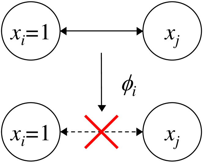
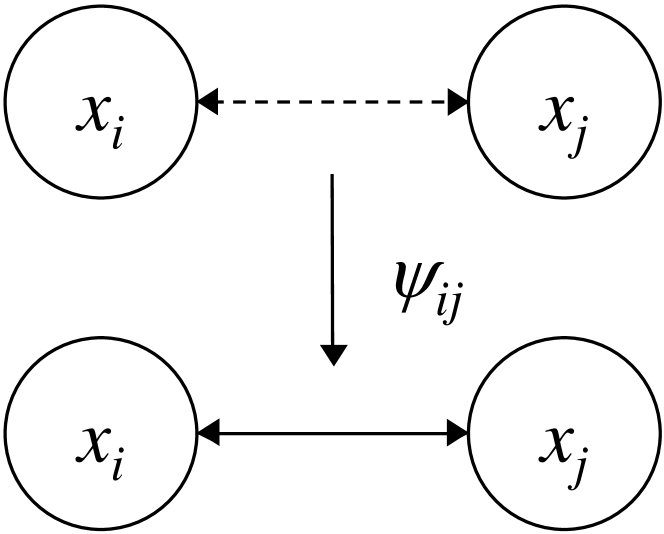
Figure 1: Adaptively switching network.

Finally, Item e) follows from the assumption that $\mathscr{G}(t)$ is undirected, although this is not an essential restriction and could be relaxed to account for directed contact networks. Also, notice that we have included the term $a_{ij}(0)$ in (4) to guarantee that only those edges that were present at the initial time $t=0$ can be added later on by the rewiring process.

Remark II.2

A model similar to the ASIS model proposed in this paper was studied in [16], where it was assumed that the initial graph $\mathscr{G}_{0}$ is the complete graph. A major difference between our model and the one in [16] is the information available to each node. In the model in [16], it is assumed that nodes know the states of their neighbors. In contrast, we do not assume to have access to this knowledge in our model. This difference has a direct implication in the link-breaking process. For example, in [16], an infected node does not break the edge between itself and its infected neighbors. On the other hand, in our model, an infected node will break edges independent of the state of its neighbors.

Once the adaptive network under consideration is described, we define the exponential stability of the infection-free equilibrium $p_{i}(t)=0$ of ASIS models, as follows:

Definition II.3

For $t\geq 0$ let $p_{i}(t)=P(x_{i}(t)=1)$ be the infection probability of node $i$. We say that the infection-free equilibrium $p_{i}(t)\equiv 0$ of the adaptive SIS model $(x,\mathscr{G})$ is exponentially stable if there exist $K\geq 0$ and $\alpha>0$ such that $p_{i}(t)\leq Ke^{-\alpha t}$ for all $i$, $t$, and $x_{i}(0)$. We call $\alpha$ the decay rate.

In many practical situations, there is a cost associated to the mechanisms of cutting and rewiring edges in a network. Accordingly, we assume we have two scalar cost functions $f$ and $g$, defined on $[0,\infty)$, describing the cost associated to the rates of cutting and rewiring edges, respectively. The main purpose of this paper is to find the cost-optimal switching strategy, defined by the values of the cutting and rewiring rates, to drive the state of the spread towards the disease-free equilibrium at a given exponential rate. The total cost of a switching strategy is given by:

$$C=\sum_{i=1}^{n}f(\phi_{i})+\smashoperator[r]{\sum_{\{i,j\}\in\mathscr{E}_{0}}^{}}\ g(\psi_{ij}).$$

We also assume the following bounds on the rates:

$$\underaccent{\bar}{\phi}\leq\phi_{i}\leq\bar{\phi},\ \underaccent{\bar}{\psi}\leq\psi_{ij}\leq\bar{\psi}$$ (5)

for some nonnegative numbers $\underaccent{\bar}{\phi}$, $\bar{\phi}$, $\underaccent{\bar}{\psi}$, and $\bar{\psi}$. Now, we are ready to state the problem investigated in this paper.

Problem II.4

Given $\alpha>0$, find the cutting and rewiring rates $\phi_{i}$ and $\psi_{ij}$ satisfying (5) such that the adaptive SIS model is exponentially stable with decay rate $\alpha$ and the total cost $C$ is minimized.

In this paper we solve Problem II.4 under the following reasonable assumption:

Assumption II.5

$\mathscr{G}_{0}$ is strongly connected. Moreover, $\beta_{i}>0$, $\delta_{i}>0$, and $\psi_{ij}>0$ for all $\{i,j\}\in\mathscr{E}_{0}$.

III Stability Analysis

In this section, we perform a stability analysis of the ASIS model $(x,\mathscr{G})$ over $\mathscr{G}_{0}$. We begin by representing the model as a set of stochastic differential equations with Poisson counters. For $\gamma\geq 0$, we let $N_{\gamma}$ denote a Poisson counter with rate $\gamma$. We assume that all Poisson counters appearing in this paper are stochastically independent. We will use superscripts for the Poisson counters to distinguish those that has the same rates but are independent. Then, from (1) and (2), the evolution of the nodal states can be described as:

$$dx_{i}=-x_{i}\,dN_{\delta_{i}}+(1-x_{i})\ \sum_{\mathclap{k\in\mathscr{N}_{i}(0)}}\ a_{ik}x_{k}\,dN_{\beta_{i}}^{(k)}.$$ (6)

Similarly, from (3) and (4), the evolution of the edges can be written as:

$$da_{ij}=-a_{ij}(x_{i}\,dN_{\phi_{i}}^{(j)}+x_{\!j}\,dN_{\phi_{\!j}}^{(i)})+(1-a_{ij})\,dN_{\psi_{ij}},$$ (7)

for all $i$ and $j$ such that $\{i,j\}\in\mathscr{E}_{0}$.

Using the stochastic differential equations (6) and (7), we derive an upper bounding linear model for the infection probabilities $p_{i}$. To state the linear model, we define the following variables. Let us define $p(t)\in\mathbb{R}^{n}$ by $p=\operatorname*{col}_{1\leq i\leq n}p_{i}$. Also, for $i=1,\dotsc,n$ and $j\in\mathscr{N}_{i}(0)$, define $q_{ij}(t)=E[a_{ij}(t)x_{i}(t)]$ and let $q_{i}=\operatorname*{col}_{j\in\mathscr{N}_{i}(0)}q_{ij}$ and $q=\operatorname*{col}_{1\leq i\leq n}q_{i}$. Let $d_{i}$ denote the degree of node $i$ in the initial graph $\mathscr{G}_{0}$ and $m$ the number of the edges in $\mathscr{G}_{0}$. Then, $q$ has the dimension $\sum_{i=1}^{N}d_{i}=2m$. We also introduce the following matrices. Define $T_{i}\in\mathbb{R}^{1\times(2m)}$ as the unique matrix satisfying:

$$T_{i}q=\sum_{k\in\mathscr{N}_{i}(0)}q_{ki}.$$ (8)

Then define the matrices $B_{1}=\operatorname*{col}_{1\leq i\leq n}(\beta_{i}T_{i})$, $B_{2}=\operatorname*{col}_{1\leq i\leq n}(\beta_{i}\mathbbold{1}_{d_{i}}\otimes T_{i})$, $D_{1}=\bigoplus_{i=1}^{n}\delta_{i}$, $D_{2}=\bigoplus_{i=1}^{n}(\delta_{i}I_{d_{i}})$, $\Phi=\bigoplus_{i=1}^{n}(\phi_{i}I_{d_{i}})$, $\Psi_{1}=\bigoplus_{i=1}^{n}\operatorname*{col}_{j\in{\mathscr{N}}_{i}(0)}\psi_{ij}$, $\Psi_{2}=\bigoplus_{i=1}^{n}\bigoplus_{{j\in\mathscr{N}_{i}(0)}}\;\psi_{ij}$. Now, we can state the following theorem:

Theorem III.1

Define $M\in\mathbb{R}^{(n+2m)\times(n+2m)}$ by

$$M=\begin{bmatrix}-D_{1}&B_{1}\\ \Psi_{1}&B_{2}-D_{2}-\Phi-\Psi_{2}\end{bmatrix}.$$ (9)

Then, for all $x_{1}(0)$, $\dotsc$, $x_{n}(0)$, it holds that

$$\frac{d}{dt}\begin{bmatrix}p\\ q\end{bmatrix}\leq M\begin{bmatrix}p\\ q\end{bmatrix}.$$ (10)

Proof:

Taking the expectations in (6) yields that

$$\frac{d}{dt}E[x_{i}]=-\delta_{i}E[x_{i}]+\beta_{i}\ \ \sum_{\mathclap{k\in\mathscr{N}_{i}(0)}}\ \ E[(1-x_{i})a_{ik}x_{k}].$$

Since $E[(1-x_{i})a_{ik}x_{k}]\leq E[a_{ik}x_{k}]=q_{ki}$, from the definition of $T_{i}$ in (8), we obtain ${dp_{i}}/{dt}\leq-\delta_{i}p_{i}+\beta_{i}T_{i}q$. This implies that $dp\!/dt\leq-D_{1}p+B_{1}q$, which proves the upper half block of the inequality (10).

Then, let us evaluate $dq/dt$. The Itô rule for jump processes [22] yields that

$$d(a_{ij}x_{i})\begin{multlined}=-a_{ij}x_{i}\,dN_{\phi_{i}}^{(j)}-a_{ij}x_{i}x_{\!j}\,dN_{\phi_{\!j}}^{(i)}+(1-a_{ij})x_{i}\,dN_{\psi_{ij}}\\ \hskip 14.22636pt-a_{ij}x_{i}\,dN_{\delta_{i}}+a_{ij}(1-x_{i})\ \sum_{\mathclap{k\in\mathscr{N}_{i}(0)}}\ a_{ik}x_{k}\,dN_{\beta_{i}}^{(k)}.\end{multlined}=-a_{ij}x_{i}\,dN_{\phi_{i}}^{(j)}-a_{ij}x_{i}x_{\!j}\,dN_{\phi_{\!j}}^{(i)}+(1-a_{ij})x_{i}\,dN_{\psi_{ij}}\\ \hskip 14.22636pt-a_{ij}x_{i}\,dN_{\delta_{i}}+a_{ij}(1-x_{i})\ \sum_{\mathclap{k\in\mathscr{N}_{i}(0)}}\ a_{ik}x_{k}\,dN_{\beta_{i}}^{(k)}.$$

Taking expectations in this equation, we obtain

$$\begin{multlined}\frac{dq_{ij}}{dt}=-\phi_{i}E[a_{ij}x_{i}]-\phi_{\!j}E[a_{ij}x_{i}x_{\!j}]+\\ \psi_{ij}E[(1-a_{ij})x_{i}]-\delta_{i}q_{ij}+\beta_{i}\ \sum_{\mathclap{k\in\mathscr{N}_{i}(0)}}\,E[a_{ij}(1-x_{i})a_{ik}x_{k}].\end{multlined}\frac{dq_{ij}}{dt}=-\phi_{i}E[a_{ij}x_{i}]-\phi_{\!j}E[a_{ij}x_{i}x_{\!j}]+\\ \psi_{ij}E[(1-a_{ij})x_{i}]-\delta_{i}q_{ij}+\beta_{i}\ \sum_{\mathclap{k\in\mathscr{N}_{i}(0)}}\,E[a_{ij}(1-x_{i})a_{ik}x_{k}].$$ (11)

Since $\sum_{k\in\mathscr{N}_{i}(0)}E[a_{ij}(1-x_{i})a_{ik}x_{k}]\leq\sum_{{k\in\mathscr{N}_{i}(0)}}E[a_{ik}x_{k}]=T_{i}q$, we obtain ${dq_{ij}}/{dt}\leq\psi_{ij}p_{i}-(\phi_{i}+\psi_{ij}+\delta_{i})q_{ij}+\beta_{i}\mathbbold{1}^{\top}_{d_{i}}T_{i}q$ from (11). Stacking the variables $q_{ij}$ for all $j\in\mathscr{N}_{i}(0)$ yields ${dq_{i}}/{dt}\leq\operatorname*{col}_{{j\in\mathscr{N}_{i}(0)}}(\psi_{ij}p_{i})-(\phi_{i}+\delta_{i})q_{i}-\psi_{j}q_{i}+\beta_{i}(\mathbbold{1}_{d_{i}}\otimes T_{i})q$, where $\psi_{j}=\bigoplus_{j\in\mathscr{N}_{i}(0)}\psi_{ji}$. This proves the lower half block of the inequality (10) and completes the proof. ∎

From Theorem III.1 we immediately have the following sufficient condition for exponential stability of the infection-free equilibrium.

Theorem III.2

If $M$ is Hurwitz stable, then the infection-free equilibrium of the adaptive SIS model is exponentially stable with a decay rate $-\eta(M)$.

Before closing this section, we prove the following proposition that plays an important role in the rest of the paper.

Proposition III.3

The matrix $M$ is irreducible.

Proof:

Define

$$L=\begin{bmatrix}O&T\\ J&S\end{bmatrix},$$

where

$$J=\bigoplus_{i=1}^{n}\mathbbold{1}_{d_{i}},\ T=\operatorname*{col}_{1\leq i\leq n}T_{i},\ S=\operatorname*{col}_{1\leq i\leq n}(\mathbbold{1}_{d_{i}}\otimes T_{i}).$$ (12)

Since $\beta_{i}$ and $\psi_{ij}$ are positive by Assumption II.5, if $M_{ij}=0$, then $L_{ij}=0$ for all distinct $i$ and $j$. From this we see that, to show the irreducibility of $M$, it is sufficient to show that $L$ is irreducible.

In order to show that $L$ is irreducible, we shall show that the directed graph $\mathscr{H}$, defined as the graph having adjacency matrix $L$, is strongly connected. We identify the nodes $1,\dotsc,n+2m$ of $\mathscr{H}$ using the variables $p_{1}$, $\dotsc$, $p_{n}$, $q_{1j}$ ($j\in\mathscr{N}_{1}(0)$), $\dotsc$, $q_{nj}$ ($j\in\mathscr{N}_{n}(0)$). Then, the upper-right block $T$ of the matrix $L$ shows that the graph $\mathscr{H}$ has directed edge $(p_{i},q_{ji})$ for all $i=1,\dotsc,n$ and $j\in\mathscr{N}_{i}(0)$. Similarly, from the matrices $J$ and $S$, we see that $\mathscr{H}$ has the edges $(q_{ij},p_{i})$ and $(q_{ij},q_{ki})$ for all $i=1,\dotsc,n$ and $j,k\in\mathscr{N}_{i}(0)$. Then, let us show that $\mathscr{H}$ has a directed path from $p_{i}$ to $p_{j}$ for all $i,j\in\{1,\dotsc,n\}$. Since $\mathscr{G}_{0}$ is strongly connected, it has a path $(i_{0},\dotsc,i_{\ell})$ such that $i_{0}=i$ and $i_{\ell}=j$. Therefore, from the above fact, we can see that $\mathscr{H}$ contains the directed path $(p_{i},q_{i_{1},i_{0}},q_{i_{2},i_{1}},\dotsc,q_{i_{\ell},i_{\ell-1}},p_{j})$. In the same way, we can show that $\mathscr{H}$ also contains the directed path $(p_{i},q_{ji},q_{ij},p_{i})$ for every $\{i,j\}\in\mathscr{E}_{0}$. These two observations show that $\mathscr{H}$ is strongly connected and, hence, $L$ is irreducible. ∎

IV Homogeneous Case

Based on the stability analysis presented in the previous section, we study the optimal design problem stated in Problem II.4. We start our analysis by assuming that the ASIS model is homogeneous, as defined below (this restriction is relaxed in the next section):

Definition IV.1

We say that the adaptive SIS model is homogeneous if there exist nonnegative constants $\beta$, $\delta$, $\phi$, and $\psi$ such that $\beta_{i}=\beta$, $\delta_{i}=\delta$, $\phi_{i}=\phi$, and $\psi_{ij}=\psi$ for all $i$ and $j$.

In the homogeneous case, the stability criterion in Theorem III.2 reduces to the next simple condition.

Theorem IV.2

Assume that the adaptive SIS model is homogeneous. Let $\rho=\eta(A_{0})$. Then, the infection-free equilibrium of the adaptive SIS model is exponentially stable if

$$\delta>\frac{\beta\rho-\phi-\psi}{2}+\frac{\sqrt{(\beta\rho+\phi+\psi)^{2}-4\beta\rho\phi}}{2}.$$ (13)

Proof:

Assume that the model is homogeneous. Then, the matrix $M$ defined in (9) takes the form

$$M=\begin{bmatrix}-\delta I&\beta T\\ \psi J&\beta S-(\delta+\phi+\psi)I\end{bmatrix},$$

where the matrices $J$, $T$, and $S$ are defined by (12). We prove the theorem under the assumption that $\beta\rho\neq\phi$. Since $\mathscr{G}_{0}$ is strongly connected by Assumption II.5, $A_{0}$ is irreducible and therefore has a positive eigenvector $v$ corresponding to the eigenvalue $\rho$ (see [23]). Define the positive vector $w=\operatorname*{col}_{1\leq i\leq n}(v_{i}\mathbbold{1}_{d_{i}})$. Then, the definition of $T_{i}$ shows $T_{i}w=\sum_{k\in\mathscr{N}_{i}(0)}w_{ki}=\sum_{k\in\mathscr{N}_{i}(0)}v_{k}=(Av)_{i}=\rho v_{i}$ and therefore $Tw=\lambda v$. In the same manner, we can show $Sw=\rho w$. Since we have $Jv=w$, for a nonnegative number $c$ it follows that

$$M\begin{bmatrix}cv\\ w\end{bmatrix}=\begin{bmatrix}(\beta\rho-c\delta)v\\ \left(c\psi+\beta\rho-(\delta+\phi+\psi)\right)w\end{bmatrix}.$$ (14)

Hence, if a real number $\lambda$ satisfies the following equations:

$$\beta\rho-c\delta=c\lambda,\ c\psi+\beta\rho-(\delta+\phi+\psi)=\lambda,$$ (15)

then, by (14), we see that the nonnegative vector $\operatorname*{col}(cv,w)$ is an eigenvector of the irreducible and Metzler matrix $M$ corresponding to the eigenvalue $\lambda$. This implies that $\eta(M)=\lambda$ (see [23, Theorem 17]). Therefore, the condition $\lambda<0$ is sufficient for exponential stability of the adaptive SIS model by Theorem III.2.

To find such $\lambda$, we solve (15) with respect to $\lambda$ and obtain $\lambda^{2}+(2\delta+\phi+\psi-\beta\rho)\lambda+\delta(\delta+\phi+\psi)-\beta\rho(\delta+\psi)=0$. This equation is satisfied by $\lambda=\lambda_{+}$, where

$$\lambda_{+}=\frac{\beta\rho-2\delta-\phi-\psi+\sqrt{(\beta\rho+\phi+\psi)^{2}-4\beta\rho\phi}}{2}.$$

Then, the pair $(c,\lambda)=(\beta\rho/(\lambda_{+}+\delta),\lambda_{+})$ satisfies (15). We remark that $\lambda_{+}+\delta$ is positive because of the initial assumption $\beta\rho\neq\phi$. Therefore, $c\geq 0$ and hence the above argument shows that

$$\eta(M)=\lambda_{+}.$$ (16)

Therefore, by Theorem III.2, the infection-free equilibrium of the adaptive SIS model is exponentially stable if $\lambda_{+}<0$, which is equivalent to (13). ∎

Remark IV.3

In the special case when the network does not adapt to the prevalence of infection, i.e., when $\phi=0$, Proposition IV.2 recovers the well-known stability condition $\delta>\beta\rho(A_{0})$ for the SIS models over static networks [2, 4].

The following theorem provides a solution to Problem II.4, in the homogeneous case:

Theorem IV.4

Assume that the adaptive SIS model is homogeneous. Let $\phi$ and $\psi$ be the solutions of the optimization problem:

$$\operatorname*{minimize}_{\phi,\psi}\ nf(\phi)+mg(\psi)$$

$$\operatorname*{subject\ to}\ \phi\geq(\beta\eta-\delta+1)\left({\psi}/{(\delta-\alpha)}+1\right),$$ (17)

$$\underaccent{\bar}{\phi}\leq\phi\leq\bar{\phi},\ \underaccent{\bar}{\psi}\leq\psi\leq\bar{\psi}.$$

Then, the pair $(\phi,\psi)$ gives the solution of Problem II.4.

Proof:

It is sufficient to show that $\eta(M)\leq-\alpha$ if and only if the (17) holds, but this easily follows from (16). ∎

V Heterogeneous Case

In this section, we extend our analysis to non-homogeneous adaptive SIS models. We will show that Problem II.4 can be effectively solved under the following assumption.

Assumption V.1

1. The values of $\psi_{ij}$ are given for every $\{i,j\}\in\mathscr{E}_{0}$;

2. There exist constants $r>\bar{\phi}$ and $s$ such that the function $F\colon[r-\bar{\phi},r-\underaccent{\bar}{\phi}]\to\mathbb{R}\colon x\mapsto s+f(r-x)$ is a posynomial function.

In order to state the main result of this section, we will need the next proposition.

Proposition V.2

Let $\bar{\delta}=\max_{i}\delta_{i}$ and define $\tilde{\delta}_{i}=\bar{\delta}-\delta_{i}$. Similarly, let $\bar{\psi}=\max_{i,j}\psi_{ij}$ and define $\tilde{\psi}_{ij}=\bar{\psi}-\psi_{ij}$. Let $\tilde{\phi}_{1}$, $\dotsc$, $\tilde{\phi}_{n}$ be real numbers. Define the matrices $\tilde{D}_{1}=\bigoplus_{i=1}^{n}\tilde{\delta}_{i}$, $\tilde{D}_{2}=\bigoplus_{i=1}^{n}(\tilde{\delta}_{i}I_{d_{i}})$, $\tilde{\Phi}=\bigoplus_{i=1}^{n}(\tilde{\phi}_{i}I_{d_{i}})$, and $\tilde{\Psi}_{2}=\bigoplus_{i=1}^{n}\bigoplus_{j\in\mathscr{N}_{i}(0)}\tilde{\psi}_{ij}$. Define the nonnegative matrix

$$\tilde{M}=\begin{bmatrix}\tilde{D}_{1}+\bar{\psi}I+rI&B_{1}\\ \Psi_{1}&B_{2}+\tilde{D}_{2}+\tilde{\Phi}+\tilde{\Psi}_{2}\end{bmatrix}.$$

Then, for a given $\alpha>0$, the following statements are equivalent:

• There exist $\phi_{1},\dotsc,\phi_{n}\in[\underaccent{\bar}{\phi},\bar{\phi}]$ such that $\eta(M)\leq-\alpha$.

• There exist $\tilde{\phi}_{1},\dotsc,\tilde{\phi}_{n}\in[r-\bar{\phi},r-\underaccent{\bar}{\phi}]$ such that $\eta(\tilde{M})+\alpha\leq{\psi_{0}}+\bar{\delta}+r$.

Moreover, between $\{\phi_{i}\}_{i=1}^{n}$ and $\{\tilde{\phi}_{i}\}_{i=1}^{n}$, there is a one-to-one correspondence given by the equation

$$\phi_{i}=r-\tilde{\phi}_{i}.$$ (18)

Proof:

Assume that there exist $\phi_{1},\dotsc,\phi_{n}\in[\underaccent{\bar}{\phi},\bar{\phi}]$ satisfying $\eta(M)\leq-\alpha$. Define $\tilde{\phi}_{i}$ by (18). Then we see that $\tilde{M}=M+(\bar{\delta}+r+\bar{\psi})I$. This implies $\eta(\tilde{M})+\alpha\leq\bar{\delta}+r+{\bar{\psi}}$. We also have $\tilde{\phi}_{i}\in[r-\bar{\phi},r-\underaccent{\bar}{\phi}]$. The other direction can be shown in the same way and, hence, its proof is omitted. ∎

Using Proposition V.2, we can reduce Problem II.4 to a geometric program under Assumption V.1, as stated in the following theorem:

Theorem V.3

Let $\tilde{\phi}_{1}$, $\dotsc$, $\tilde{\phi}_{n}$ be the solutions to the following geometric program:

$$\operatorname*{minimize}_{\tilde{\phi_{i}},\,v}\ \sum_{i=1}^{n}F(\tilde{\phi}_{i})$$ (19a)

$$\operatorname*{subject\ to}\ \left(\tilde{M}+\alpha I\right)v\leq\left(\bar{\delta}+r+\bar{\psi}\right)v,\hskip 14.22636pt$$ (19b)

$$\phantom{\operatorname*{subject\ to}}\ v>0,$$ (19c)

$$\phantom{\operatorname*{subject\ to}}\ r-\bar{\phi}\leq\tilde{\phi}_{i}\leq r-\underaccent{\bar}{\phi}.$$ (19d)

Then, $\{\phi_{i}\}_{i=1}^{n}$, defined in (18) solve Problem II.4.

Proof:

By Proposition V.2, Problem II.4 is equivalent to the optimization problem

$$\operatorname*{minimize}_{\tilde{\phi}_{i}}\ \sum_{i=1}^{n}f(r-\tilde{\phi_{i}})$$

$$\operatorname*{subject\ to}\ \eta(\tilde{M}+\alpha I)\leq\bar{\delta}+r+{\bar{\psi}},$$ (20)

$$r-\bar{\phi}\leq\tilde{\phi}_{i}\leq r-\underaccent{\bar}{\phi},$$

after the change of variables (18). Minimizing the objective function in this problem is equivalent to minimizing the one in (19) by the definition of $F$, whose constant term $s$ can be ignored in the optimization. Then, since $\tilde{M}+\alpha I$ is irreducible by Proposition III.3, we can replace the constraint (20) into (19b) and (19c) in the same way as in [8] using Perron-Frobenius lemma. Also, by a similar argument as in [8], we can show that (19) is a geometric program. This is because $F$ is a posynomial and each entry of the matrix $\tilde{M}+\alpha I$ is a posynomial in the variables $\tilde{\phi}_{1}$, $\dotsc$, $\tilde{\phi}_{n}$. The details are omitted. ∎

Remark V.4

When $\psi_{ij}$ are also design variables, the above argument reduces Problem II.4 to a signomial program, which are (in general) hard to solve [20].

VI Numerical Results

We illustrate our results with a numerical example. Let $\mathscr{G}_{0}$ be the graph of a social network of $n=247$ nodes and $m=940$ edges. The adjacency matrix of the graph has spectral radius $\rho=13.53$. We assume that all nodes have identical recovery rate $\delta=0.1$ and infection rate $\beta=\delta/(1.1\rho)=6.720\times 10^{-3}$. Since $\delta/\beta=(1.1)\rho>\rho$, Theorem IV.2 does not guarantee the stability of the infection-free equilibrium when $\phi=0$, i.e., when the network does not adapt.

Let us design the cost-optimal cutting rates so that the spread stabilizes towards the disease-free equilibrium in the adaptive network. We assume $\underaccent{\bar}{\phi}=0$, $\bar{\phi}=4\beta$, and $\psi_{ij}=\beta$ and use the following cost function in our numerical simulations:

$$f(x)=\frac{(r-x)\mathstrut^{-1}-(r-\underaccent{\bar}{\phi})^{-1}}{(r-\bar{\phi})^{-1}-(r-\underaccent{\bar}{\phi})^{-1}}.$$

We have chosen this function since it is increasing and presents diminishing returns. Also, we have normalized it, so that $f(\underaccent{\bar}{\phi})=0$ and $f(\bar{\phi})=1$, and fixed $r=2\bar{\phi}$. Let the desired exponential decay rate be $\alpha=0.005$ and solve the geometric program in Theorem IV.4 to obtain the optimal cutting rates $\phi_{i}$. Fig. 2 shows a scatter plot for the optimal rates, $\phi_{i}$, versus the degrees of the nodes for all $i\in\mathscr{V}$.

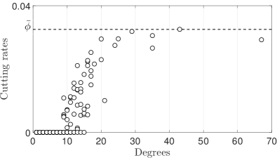
Figure 2: Cost-optimal cutting rates for stabilization

The resulting switching policy suggests that, in general, nodes with a larger degree should have higher cutting rates (as could be naturally expected). However, the relationship between the optimal cutting rates and the degrees is not trivial. Alternatively, we have also studied the relationship between cutting rates and other network centrality measures and $K$-scores (though we omit these figures for space limitations). Our simulations do not show any trivial dependency between cutting rates and any of the measures considered.

VII Conclusion

In this paper, we have studied the dynamics of spreading processes taking place in networks that adapt their structure depending on the state of the dynamics. Our model is based on a collection of stochastic differential equations with Poisson jumps that model the joint evolution of the states of the process taking place in the network, as well as the evolution of the network structure. To illustrate our framework, we have focused our attention in a popular model of spreading dynamics, the SIS model, and study it dynamics over adaptive, switched networks. For this particular model, we have derived conditions for the dynamics of the spread to converge towards the disease-free equilibrium. Using this stability result, we have then formulated an optimization program to find the cost-optimal adaptive strategy to achieve stability. We have also showed that this optimization program can be efficiently solved using geometric programming. A numerical example was included to illustrate our results. An interesting future work is to fully investigate the difference of information structures in our model and the one in [16] addressed in Remark II.2.

References

- [1] R. Pastor-Satorras, C. Castellano, P. Van Mieghem, and A. Vespignani, “Epidemic processes in complex networks,” Reviews of Modern Physics, vol. 87, pp. 925–979, 2015.
- [2] A. Lajmanovich and J. A. Yorke, “A deterministic model for gonorrhea in a nonhomogeneous population,” Mathematical Biosciences, vol. 28, pp. 221–236, 1976.
- [3] D. Chakrabarti, Y. Wang, C. Wang, J. Leskovec, and C. Faloutsos, “Epidemic thresholds in real networks,” ACM Transactions on Information and System Security, vol. 10, 2008.
- [4] P. Van Mieghem, J. Omic, and R. Kooij, “Virus spread in networks,” IEEE/ACM Transactions on Networking, vol. 17, pp. 1–14, 2009.
- [5] V. M. Preciado, M. Zargham, C. Enyioha, A. Jadbabaie, and G. Pappas, “Optimal vaccine allocation to control epidemic outbreaks in arbitrary networks,” in 52nd IEEE Conference on Decision and Control, 2013, pp. 7486–7491.
- [6] V. M. Preciado, F. D. Sahneh, and C. Scoglio, “A convex framework for optimal investment on disease awareness in social networks,” in 2013 IEEE Global Conference on Signal and Information Processing, 2013, pp. 851–854.
- [7] V. M. Preciado and M. Zargham, “Traffic optimization to control epidemic outbreaks in metapopulation models,” in 2013 IEEE Global Conference on Signal and Information Processing, 2013, pp. 847–850.
- [8] V. M. Preciado, M. Zargham, C. Enyioha, A. Jadbabaie, and G. J. Pappas, “Optimal resource allocation for network protection against spreading processes,” IEEE Transactions on Control of Network Systems, vol. 1, pp. 99–108, 2014.
- [9] D. Bell, A. Nicoll, K. Fukuda, P. Horby, A. Monto, F. Hayden, C. Wylks, L. Sanders, and J. Van Tam, “Nonpharmaceutical interventions for pandemic influenza, national and community measures,” Emerging Infectious Diseases, vol. 12, pp. 88–94, 2006.
- [10] S. Funk, M. Salathé, and V. A. A. Jansen, “Modelling the influence of human behaviour on the spread of infectious diseases: a review.” Journal of the Royal Society, Interface / the Royal Society, vol. 7, pp. 1247–1256, 2010.
- [11] E. Volz and L. A. Meyers, “Epidemic thresholds in dynamic contact networks.” Journal of the Royal Society, Interface / the Royal Society, vol. 6, pp. 233–241, 2009.
- [12] N. Perra, B. Gonçalves, R. Pastor-Satorras, and A. Vespignani, “Activity driven modeling of time varying networks.” Scientific reports, vol. 2:469, 2012.
- [13] M. Ogura and V. M. Preciado, “Optimal design of switched networks of positive linear systems via geometric programming,” IEEE Transactions on Control of Network Systems (Accepted), 2015.
- [14] T. Gross, C. J. D. D’Lima, and B. Blasius, “Epidemic dynamics on an adaptive network,” Physical Review Letters, vol. 96, p. 208701, 2006.
- [15] D. H. Zanette and S. Risau-Gusmán, “Infection spreading in a population with evolving contacts,” Journal of Biological Physics, vol. 34, pp. 135–148, 2008.
- [16] D. Guo, S. Trajanovski, R. van de Bovenkamp, H. Wang, and P. Van Mieghem, “Epidemic threshold and topological structure of susceptible-infectious-susceptible epidemics in adaptive networks,” Physical Review E, vol. 88, p. 042802, 2013.
- [17] I. Tunc and L. B. Shaw, “Effects of community structure on epidemic spread in an adaptive network,” Physical Review E, vol. 90, p. 022801, 2014.
- [18] L. D. Valdez, P. A. Macri, and L. A. Braunstein, “Intermittent social distancing strategy for epidemic control,” Physical Review E, vol. 85, p. 036108, 2012.
- [19] P. Holme and N. Masuda, “The basic reproduction number as a predictor for epidemic outbreaks in temporal networks,” PLOS ONE, vol. 10, p. e0120567, 2015.
- [20] S. Boyd, S.-J. Kim, L. Vandenberghe, and A. Hassibi, “A tutorial on geometric programming,” Optimization and Engineering, vol. 8, pp. 67–127, 2007.
- [21] J. Brewer, “Kronecker products and matrix calculus in system theory,” IEEE Transactions on Circuits and Systems, vol. 25, pp. 772–781, 1978.
- [22] R. W. Brockett, “Stochastic Control,” 2008.
- [23] L. Farina and S. Rinaldi, Positive Linear Systems: Theory and Applications. Wiley-Interscience, 2000.