Enhancements of Andreev conductance induced by the photon/vibron scattering

Abstract

We analyze the subgap spectrum and transport properties of the quantum dot embedded between one superconducting and another metallic reservoirs and additionally coupled to an external boson mode. Emission/absorption of the bosonic quanta induces a series of the subgap Andreev states, that eventually interfere with each other. We discuss their signatures in the differential conductance both, for the linear and nonlinear regimes.

I Introduction

The bosonic modes, like photons Platero_Aguado_2004 or vibrational degrees of freedom Galperin_2007 , can strongly affect electron tunneling through the nanoscopic systems Koch_2005 . When a level spacing of nanoobject is large in comparison to the boson energy $\omega_{0}$ and a line-broadening is sufficiently narrow, a series of the side-peaks Fransson_book may appear due to emission/absorption of the bosonic quanta. Such features (spaced by $\omega_{0}$) have been really observed in measurements of the differential conductance for several nanojunctions Sapmaz_2006 ; Leturcq_2009 ; Beebe_2006 ; Pasupathy_2005 .

Similar bosonic modes are currently studied also in the systems, where the quantum dots/impurities are coupled with superconducting reservoirs Cho_1999 ; Song_2008 ; Zazunov_2006 ; Fransson_2010 ; Timm_2012 ; Zhang_2009 ; Bai_2011 ; Sun_2012 ; Zitko_2012 ; Rudzinski_2014 ; Komnik_13 ; Wang_2013 . Since the proximity effect spreads electron pairing onto these quantum dots, the bosonic features manifest themselves in a quite peculiar way. They could be observed by the Josephson Zazunov_2006 ; Fransson_2010 ; Timm_2012 and the Andreev spectroscopies Cho_1999 ; Zhang_2009 ; Bai_2011 ; Sun_2012 ; Zitko_2012 ; Rudzinski_2014 , in photon-assisted subgap tunneling Song_2008 , transient phenomena Komnik_13 , or in prototypes of the nano-refrigerators operating due to the multi-phonon Andreev scattering Wang_2013 .

First of all, in a subgap regime (assuming $\omega_{0}$ smaller than energy gap $\Delta$ of superconductor) the bosonic features are expected to be more numerous than in the normal state. This is a consequence the proximity effect, mixing the particle and hole excitations. Secondly, it has been shown numerically Cho_1999 ; Sun_2012 ; Wang_2013 that the linear (zero-bias) Andreev conductance exhibits the bosonic features spaced by a half of $\omega_{0}$. To our knowledge, this intriguing theoretical result was neither clarified on physical arguments nor checked experimentally. Verification would be feasible by the tunneling spectroscopy using e.g. low-frequency vibrations of some heavy molecules or slowly-varying ac electromagnetic field. Let us emphasize, that such low-energy boson mode need not be related with any pairing mechanism of the superconducting reservoir.

The purpose of our paper is to provide a simple analytical argument, explaining the reduced frequency $\omega_{0}/2$ of the bosonic features in the linear Andreev conductance versus the gate-voltage. We also study in detail the multiple subgap states originating from the boson emission/absorption processes. We analyze their signatures both in the quantum dot spectrum and the tunneling transmission. The latter quantity can be probed by the (low-temperature) differential conductance as a function of the source-drain bias. We predict that the multiple Andreev states could be seen with a period, dependent on the gate voltage.

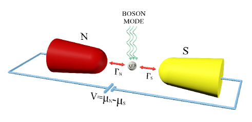
Figure 1: (color online) A scheme of the quantum dot between the metallic (N) and superconducting (S) electrodes and coupled to the monochromatic boson (phonon or photon) mode.

For calculations we consider the setup displayed in figure 1. It can be practically realized in a single electron transistor (SET) using e.g. the carbon nanotube suspended between the external electrodes (like in Refs Sapmaz_2006 ; Leturcq_2009 ). Another possibility could be the scanning tunneling microscope (STM), where the conducting tip (N) probes some vibrating quantum impurity (QD) hosted in a superconducting (S) substrate Balatsky-06 . In both SET and STM configurations such boson mode can be eventually related to external ac field.

In what follows we introduce the Hamiltonian and discuss the method for treating the bosonic mode. We next investigate the bosonic signatures in the QD spectrum and in the subgap Andreev conductance. For clarity, we focus on the limit $\Gamma_{N}\ll\omega_{0}$ whereas the second coupling $\Gamma_{S}$ can be arbitrary. In the last section we address the correlation effects.

II Microscopic model

For microscopic description of the tunneling scheme shown in Fig. 1 we use the Anderson impurity model

$$\hat{H}=\hat{H}_{N}+\hat{H}_{S}+\hat{H}_{mol}+\hat{H}_{T}.$$ (1)

$\hat{H}_{N(S)}$ refers to the normal (superconducting) lead, $\hat{H}_{mol}$ describes the molecular quantum dot (i.e. the localized electrons coupled with the boson mode) and $\hat{H}_{T}$ is a hybridization between the QD and itinerant electrons. We treat the normal electrode as a free Fermi gas $\hat{H}_{N}=\sum_{{\bf k},\sigma}\xi_{{\bf k}N}\hat{c}_{{\bf k}\sigma N}^{\dagger}\hat{c}_{{\bf k}\sigma N}$ and describe the other superconducting lead by the BCS Hamiltonian $\hat{H}_{S}\!=\!\sum_{{\bf k},\sigma}\xi_{{\bf k}S}\hat{c}_{{\bf k}\sigma S}^{\dagger}\hat{c}_{{\bf k}\sigma S}\!-\!\Delta\sum_{\bf k}(\hat{c}_{{\bf k}\uparrow S}^{\dagger}\hat{c}_{-{\bf k}\downarrow S}^{\dagger}\!+\!\hat{c}_{-{\bf k}\downarrow S}\hat{c}_{{\bf k}\uparrow S})$. The annihilation (creation) operators $\hat{c}_{{\bf k}\sigma\beta}^{({\dagger})}$ correspond to mobile $\beta=N,S$ electrons with spin $\sigma=\uparrow,\downarrow$ and energy $\xi_{{\bf k}\beta}\!=\!\varepsilon_{{\bf k}\beta}\!-\!\mu_{\beta}$ measured with respect to the chemical potential $\mu_{\beta}$. Nonequlibrium conditions can be driven by the bias $V=\mu_{L}-\mu_{R}$ and/or temperature difference $T_{L}\neq T_{R}$. The induced currents depend qualitatively on the hybridization $\hat{H}_{T}=\sum_{{\bf k},\sigma,\beta}\left(V_{{\bf k}\beta}\;\hat{d}_{\sigma}^{\dagger}\hat{c}_{{\bf k}\sigma\beta}+\mbox{\rm H.c.}\right)$ and on parameters of the molecular quantum dot

$$\hat{H}_{mol}=\varepsilon\sum_{\sigma}\hat{n}^{\dagger}_{d\sigma}+U\hat{n}_{d\uparrow}\hat{n}_{d\downarrow}+\omega_{0}\hat{a}^{\dagger}\hat{a}+\lambda\sum_{\sigma}\hat{n}_{d\sigma}(\hat{a}^{\dagger}\!+\hat{a}).$$

The number operator $\hat{n}_{d\sigma}=\hat{d}^{\dagger}_{\sigma}\hat{d}_{\sigma}$ counts the localized electrons with spin $\sigma$, $\varepsilon$ is the QD energy level and $U$ denotes the Coulomb potential between opposite spin electrons. The boson field (described by $\hat{a}^{(\dagger)}$ operators) is assumed as a monochromatic mode $\omega_{0}$ and its coupling with the QD electrons is denoted by $\lambda$.

III Multiple subgap states

There are three main obstacles in determining the effective energy spectrum and the tunneling transmission of our system: i) the electron-boson coupling $\lambda$, ii) the proximity induced on-dot pairing (due to $\Delta$), and iii) the correlation effects caused by the Coulomb repulsion $U$. The most reliable way for studying them on equal footing would be possible within the numerical renormalization group Zitko_2012 approach, however such method encounters problems in estimating the Andreev transmission. To get some insight into the spectrum and transport properties we start by neglecting the correlations and then (in the last section) treat them using the superconducting atomic limit solution.

Following Cho_1999 ; Song_2008 ; Zazunov_2006 ; Fransson_2010 ; Timm_2012 ; Zhang_2009 ; Bai_2011 ; Sun_2012 ; Zitko_2012 ; Rudzinski_2014 ; Wang_2013 we apply the unitary transformation $e^{\hat{S}}\hat{H}e^{-\hat{S}}=\hat{\tilde{H}}$ to decouple the electron from boson quasiparticles. With the Lang-Firsov generating operator Lang_Firsov

$$\hat{S}=\frac{\lambda}{\omega_{0}}\sum_{\sigma}\hat{n}_{d\sigma}\left(\hat{a}^{\dagger}-\hat{a}\right)$$ (2)

the molecular Hamiltonian (II) is transformed to

$$\hat{\tilde{H}}_{mol}=\sum_{\sigma}\tilde{\varepsilon}\hat{\tilde{d}}_{\sigma}^{\dagger}\hat{\tilde{d}}_{\sigma}+\tilde{U}\hat{\tilde{n}}_{\downarrow}\hat{\tilde{n}}_{\uparrow}+\omega_{0}\hat{a}^{\dagger}\hat{a},$$ (3)

where the energy level is lowered by the polaronic shift $\tilde{\epsilon}=\varepsilon\!-\!\lambda^{2}/\omega_{0}$ and the effective potential $\tilde{U}\!=\!U-2\lambda^{2}/\omega_{0}$. Boson operators are shifted $\hat{\tilde{a}}^{(\dagger)}=\hat{a}^{(\dagger)}-\frac{\lambda}{\omega_{0}}\sum_{\sigma}\hat{d}_{\sigma}^{\dagger}\hat{d}_{\sigma}$ whereas fermions are dressed with the polaronic cloud

$$\hat{\tilde{d}}_{\sigma}^{(\dagger)}=\hat{d}_{\sigma}^{(\dagger)}\hat{X}^{(\dagger)},\hskip 28.45274pt\hat{X}=e^{-(\lambda/\omega_{0})(\hat{a}^{\dagger}-\hat{a})}.$$ (4)

Reservoirs $\hat{H}_{\beta}$ are invariant on the unitary transformation (2) but the operator $\hat{X}$ appears in the hybridization term $\hat{\tilde{H}}_{T}$. For simplicity we absorb it into the effective coupling constants $\Gamma_{\beta}=2\pi\sum_{\bf k}|V_{{\bf k}\beta}|^{2}\;\langle\hat{X}^{\dagger}\hat{X}\rangle\delta(\omega\!-\!\xi_{{\bf k}\beta})$ which can be defined for the wide band limit.

The effective single particle excitation spectrum is given by the Green’s function

$${\mbox{\boldmath{$G$}}}_{\sigma}(\tau_{1},\tau_{2})=-i\;\left\langle\hat{T}_{\tau}\hat{d}_{\sigma}(\tau_{1})\hat{d}_{\sigma}^{\dagger}(\tau_{2})\right\rangle_{\hat{H}},$$ (5)

where $\hat{T}_{\tau}$ denotes the time ordering operator. Since trace is invariant on the unitary transformations $\langle...\rangle_{\hat{H}}=\langle...\rangle_{\hat{\tilde{H}}}$ it is convenient to compute the statistical averages with respect to $\hat{\tilde{H}}$. In particular, (5) can be expressed as

$${\mbox{\boldmath{$G$}}}_{\sigma}(\tau_{1},\tau_{2})=-i\left\langle\hat{T}_{\tau}\hat{d}_{\sigma}(\tau_{1})\hat{d}_{\sigma}^{\dagger}(\tau_{2})\right\rangle_{\hat{\tilde{H}}_{fer}}\!\!\left\langle\hat{T}_{\tau}\hat{X}(\tau_{1})\hat{X}^{\dagger}(\tau_{2})\right\rangle_{\hat{\tilde{H}}_{bos}}$$ (6)

because the fermionic and bosonic degrees of freedom are separated by the Lang-Firsov transformation. From a standard procedure Fransson_book ; Mahan_book one obtains

$$\left\langle\hat{T}_{\tau}\hat{X}(\tau_{1})\hat{X}(\tau_{2})^{\dagger}\right\rangle_{\hat{\tilde{H}}_{bos}}=\mbox{\rm exp}\left\{-(\lambda/\omega_{0})^{2}\right.\;\times$$ (7)

$$\left.[(1-e^{-i\omega_{0}(\tau_{1}-\tau_{2})})(1+N_{p})+(1-e^{i\omega_{0}(\tau_{1}-\tau_{2})})N_{p}]\right\}$$

with the Bose-Einstein distribution $N_{p}=\left[e^{\beta\omega_{0}}-1\right]^{-1}$. Fourier transform of the Green’s function (7) is found as

$${\mbox{\boldmath{$G$}}}_{\sigma}(\omega) = \sum_{l}{\mbox{\boldmath{$g$}}}_{\sigma}(\omega\!-\!l\omega_{0})\;\;e^{-(\lambda\sqrt{1+2N_{p}}/\omega_{0})^{2}}$$

$$\times e^{l\beta\omega_{0}/2}I_{l}\left[2(\frac{\lambda}{\omega_{0}})^{2}\sqrt{N_{p}(1+N_{p})}\right],$$

where $I_{l}$ denote the modified Bessel functions and ${\mbox{\boldmath{$g$}}}_{\sigma}(\tau_{1},\tau_{2})=-i\left\langle\hat{T}_{\tau}\hat{d}_{\sigma}(\tau_{1})\hat{d}_{\sigma}^{\dagger}(\tau_{2})\right\rangle_{\hat{\tilde{H}}_{fer}}$ is the fermionic part of (6). In the ground state (III) simplifies to

$$\lim_{T\rightarrow 0}{\mbox{\boldmath{$G$}}}_{\sigma}(\omega)=\sum_{l}{\mbox{\boldmath{$g$}}}_{\sigma}(\omega\!-\!l\omega_{0})\;\;e^{-g}\;\frac{g^{l}}{l!}$$ (9)

with the adiabatic parameter $g=(\lambda/\omega_{0})^{2}$.

Due to the proximity induced on-dot pairing the single particle Green’s function ${\mbox{\boldmath{$G$}}}_{\uparrow}(\tau_{1},\tau_{2})$ is mixed with the (anomalous) propagator

$${\mbox{\boldmath{$F$}}}(\tau_{1},\tau_{2})=-i\left\langle\hat{T}_{\tau}\hat{d}_{\downarrow}^{\dagger}(\tau_{1})\hat{d}_{\uparrow}^{\dagger}(\tau_{2})\right\rangle_{\hat{H}}=$$ (10)

$$-i\left\langle\hat{T}_{\tau}\hat{d}_{\downarrow}^{\dagger}(\tau_{1})\hat{d}_{\uparrow}^{\dagger}(\tau_{2})\right\rangle_{\hat{\tilde{H}}_{fer}}\left\langle\hat{T}_{\tau}\hat{X}^{\dagger}(\tau_{1})\hat{X}^{\dagger}(\tau_{2})\right\rangle_{\hat{\tilde{H}}_{bos}}.$$

This important fact has been remarked in the previous considerations of dc Josephson current Timm_2012 and it also plays significant role for the Andreev spectroscopy (see the next section). The boson part of the anomalous propagator (10) takes the following form

$$\left\langle\hat{T}_{\tau}\hat{X}^{\dagger}(\tau_{1})\hat{X}(\tau_{2})^{\dagger}\right\rangle_{bos}=\mbox{\rm exp}\left\{-(\lambda/\omega_{0})^{2}\right.\;\times$$ (11)

$$\left.[(1+e^{-i\omega_{0}(\tau_{1}-\tau_{2})})(1+N_{p})+(1+e^{i\omega_{0}(\tau_{1}-\tau_{2})})N_{p}]\right\}.$$

At zero temperature its Fourier transform simplifies to

$$\lim_{T\rightarrow 0}{\mbox{\boldmath{$F$}}}(\omega)=\sum_{l}{\mbox{\boldmath{$f$}}}(\omega\!-\!l\omega_{0})\;\;e^{-g}\;\frac{(-g)^{l}}{l!}.$$ (12)

As regards the fermion part ${\mbox{\boldmath{$f$}}}(\tau_{1},\tau_{2})=-i\langle\hat{T}_{\tau}\hat{d}^{\dagger}_{\downarrow}(\tau_{1})\hat{d}_{\uparrow}^{\dagger}(\tau_{2})\rangle_{\hat{\tilde{H}}_{fer}}$ it couples to the Green’s function ${\mbox{\boldmath{$g$}}}(\tau_{1},\tau_{2})$. Their Fourier components obey the Dyson equation

$$\left[\begin{array}[]{cc}{\mbox{\boldmath{$g$}}}(\omega)&{\mbox{\boldmath{$f$}}}(\omega)\\ {\mbox{\boldmath{$f$}}}^{\star}(-\omega)&-{\mbox{\boldmath{$g$}}}^{\star}(-\omega)\end{array}\right]^{-1}$$ (15)

$$= \left[\begin{array}[]{cc}\omega\!-\!\tilde{\varepsilon}&0\\ 0&\omega\!+\!\tilde{\varepsilon}\end{array}\right]-{{\mbox{\boldmath{$\Sigma$}}}}_{QD}^{0}(\omega)-{{\mbox{\boldmath{$\Sigma$}}}}_{QD}^{corr}(\omega),$$ (18)

where ${{\mbox{\boldmath{$\Sigma$}}}}_{d}^{0}$ is the selfenergy matrix of uncorrelated molecular dot and the second contribution ${{\mbox{\boldmath{$\Sigma$}}}}_{d}^{corr}$ is due to the effective Coulomb interaction $\tilde{U}$. In the wide-band limit the selfenergy ${{\mbox{\boldmath{$\Sigma$}}}}_{QD}^{0}(\omega)$ can be expressed as

$${\mbox{\boldmath{$\Sigma$}}}_{QD}^{0}(\omega)=-i\frac{\Gamma_{N}}{2}\;\left(\begin{array}[]{cc}1&0\\ 0&1\end{array}\right)-\frac{\Gamma_{S}}{2}\gamma(\omega)\left(\begin{array}[]{cc}1&\frac{\Delta}{\omega}\\ \frac{\Delta}{\omega}&1\end{array}\right)$$ (23)

with

$$\gamma(\omega)=\left\{\begin{array}[]{ll}\frac{\omega}{\sqrt{\Delta^{2}-\omega^{2}}}&\mbox{\rm for }|\omega|<\Delta,\\ \frac{i\;|\omega|}{\sqrt{\omega^{2}-\Delta^{2}}}&\mbox{\rm for }|\omega|>\Delta.\end{array}\right.$$ (26)

We investigated the effective spectral function $\rho(\omega)=-\pi^{-1}\mbox{\rm Im}{\mbox{\boldmath{$G$}}}(\omega+i0^{+})$ at zero temperature, focusing on the intermediate electron-boson coupling $g\sim 1$. Figures 2–4 show the QD spectrum for $\tilde{U}\!=\!0$, neglecting the correlation effects ${{\mbox{\boldmath{$\Sigma$}}}}_{d}^{corr}$. Influence of the Coulomb potential $\tilde{U}$ is discussed in section V.

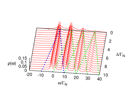
Figure 2: (color online) Energy spectrum $\rho(\omega)$ of the uncorrelated quantum dot ($\tilde{U}\!=\!0)$ obtained at $T=0$ for $\tilde{\varepsilon}=0$, $g=1$, $\omega_{0}=10\Gamma_{N}$. The filled triangles at $l\omega_{0}\pm\Delta$ are only guide to eye. For increasing $\Delta$ the boson peaks split into the lower and upper states and their broadening shrinks to $\Gamma_{N}$.

Fig 2 illustrates evolution of the bosonic features with respect to the superconductor gap $\Delta$. In the normal state (for $\Delta=0$) such lorentzian peaks are located at $\omega=\tilde{\varepsilon}+l\omega_{0}$ (with integer $l\geq 0$) and their broadening is $\Gamma_{N}+\Gamma_{S}$. For finite $\Delta$ all peaks split into the lower and upper ones due to the induced on-dot pairing. In the extreme limit $\Delta\gg\Gamma_{S}$ the selfenergy ${\mbox{\boldmath{$\Sigma$}}}_{QD}^{0}(\omega)$ becomes static

$$\lim_{\Delta\gg\Gamma_{S}}{\mbox{\boldmath{$\Sigma$}}}_{QD}^{0}(\omega)=-\;\frac{1}{2}\;\left(\begin{array}[]{cc}i\Gamma_{N}&\Gamma_{S}\\ \Gamma_{S}&i\Gamma_{N}\end{array}\right)$$ (29)

therefore the effective quasiparticle energies evolve to $l\omega_{0}\pm\sqrt{\tilde{\varepsilon}^{2}+(\Gamma_{S}/2)^{2}}$ and their broadening shrinks to $\Gamma_{N}$.

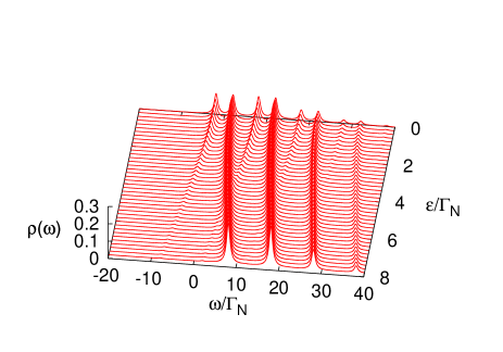
Figure 3: (color online) Spectrum of the uncorrelated quantum dot for $\omega_{0}=10\Gamma_{N}$, $g=1$, $\Gamma_{S}=4\Gamma_{N}$, $T=0$. The neighboring boson peaks are crossing at $\omega=(\frac{1}{2}+l)\omega_{0}$ for $\tilde{\varepsilon}\simeq\omega_{0}/2$.

Focusing on such superconducting atomic limit (29) we show in Fig. 4 the subgap bosonic peaks with respect to $\tilde{\varepsilon}$. In the SET configuration the energy level $\tilde{\varepsilon}$ would be tunable by applying the gate voltage. In particular, these peaks may overlap with each other when $\tilde{\varepsilon}\simeq\omega_{0}/2$ as reported earlier in the Refs Cho_1999 ; Sun_2012 ; Wang_2013 . This effect can be deduced analytically from

$$l\omega_{0}+\sqrt{\tilde{\varepsilon}^{2}+(\Gamma_{S}/2)^{2}}=l^{\prime}\omega_{0}-\sqrt{\tilde{\varepsilon}^{2}+(\Gamma_{S}/2)^{2}}.$$ (30)

The neighboring peaks ($l^{\prime}\!=\!l\!+\!1$) overlap when $\omega_{0}/2=\sqrt{\tilde{\varepsilon}^{2}+(\Gamma_{S}/2)^{2}}$. For small $\Gamma_{S}$ such situation takes place at $\tilde{\varepsilon}\simeq\frac{1}{2}\omega_{0}$. Other crossings would be eventually possible for the higher-order multiplications of $\omega_{0}/2$.

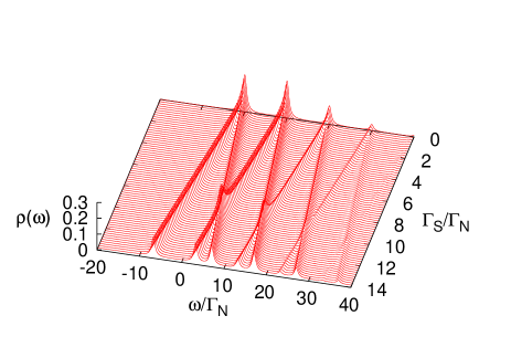
Figure 4: (color online) Spectrum of the uncorrelated quantum dot for $\tilde{\varepsilon}=0$, $g=1$, $\omega_{0}=10\Gamma_{N}$, $T=0$, $\Delta\gg\Gamma_{S}$. The bosonic features cross each other at $\omega=(\frac{1}{2}+l)\omega_{0}$ for $\Gamma_{S}=\omega_{0}$.

Figure 4 displays the subgap spectrum $\rho(\omega)$ as a function of the coupling $\Gamma_{S}$. From (30) we conclude that for $\tilde{\varepsilon}=0$ the bosonic peaks overlap at $\Gamma_{S}=\omega_{0}$. Energy of these crossing points is $\omega=(\frac{1}{2}+l)\omega_{0}$. Here (for $g=1$) we observe four such crossings, but for stronger electron-boson couplings a number of the in-gap states and their crossings would increase.

IV Andreev conductance

Under nonequilibrium conditions the charge current can be transmitted at small voltage $|eV|\!<\!\Delta$ via the Andreev scattering, engaging the in-gap states. This anomalous transport channel occurs when electrons from the metallic lead are converted into the Cooper pairs (propagating in superconducting electrode) with the holes reflected back to $N$ electrode. The resulting current $I_{A}(V)$ can be expressed by the Landauer-type formula transport_formula

$$I_{A}(V)=\frac{2e}{h}\int\!\!d\omega\;T_{A}(\omega)\left[f_{FD}(\omega\!-\!eV)\!-\!f_{FD}(\omega\!+\!eV)\right],$$ (31)

with the Fermi-Dirac function $f_{FD}(\omega)=\left[e^{\omega/k_{B}T}+1\right]^{-1}$ and the Andreev transmittance transport_formula

$$T_{A}(\omega)=\Gamma_{N}^{2}\;\left|{{\mbox{\boldmath{$F$}}}}(\omega)\right|^{2}.$$ (32)

Optimal conditions for this subgap transmittance occur when $\omega$ coincides with the subgap quasiparticle states. In our present case we thus expect a number of such enhancements due the bosonic features. Let’s remark that $T_{A}(-\omega)\!=\!T_{A}(\omega)$ implies the Andreev conductance $G_{A}(V)=\frac{\partial I_{A}(V)}{\partial V}$ to be an even function of the bias $V$.

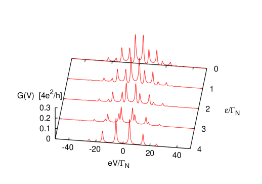
Figure 5: (color online) The differential Andreev conductance $G_{A}(V)$ versus the source-drain voltage $V$ and the QD level $\varepsilon$ (tunable by the gate voltage). Results are obtained for $T=0$, $g=1$, $\Gamma_{S}/\Gamma_{N}$=6, $\omega_{0}/\Gamma_{N}=10$, $\tilde{U}=0$ and $\Delta\gg\Gamma_{S}$. Conductance is expressed in units of $4e^{2}/h$.

Fig. 5 shows the Andreev conductance as a function of voltage $V$ applied between the metallic and superconducting electrodes. We notice the differential conductance enhancements whenever $V$ coincides with the in-gap quasiparticle energies. Since $T_{A}(-\omega)\!=\!T_{A}(\omega)$ we observe these maxima at $\pm\sqrt{\tilde{\varepsilon}^{2}+(\Gamma_{S}/2)^{2}}\pm l\omega_{0}$. They eventually overlap when (30) is satisfied. In particular, for $\Gamma_{S}=6\Gamma_{N}$ and $\omega_{0}=10\Gamma_{N}$ the nearest bosonic peaks overlap when $\tilde{\varepsilon}=4\Gamma_{N}$. Figure 5 clearly shows that the resulting maxima appear at $|eV|=\omega_{0}(1/2+l)$.

V Correlation effects

In various experimental realizations of the quantum dots (such as self-assembled InAs islands Deacon-10 , carbon nanotubes Pillet2013 ; Schindele2014 or semiconducting nanowires Lee2012 ; Lee2014 ) attached to the superconducting leads the energy gap $\Delta$ was safely smaller than the repulsion potential $U$. For this reason, in the subgap Andreev spectroscopy the correlations hardly contributed any Coulomb blockade. Instead of it, they can eventually induce the singlet-doublet quantum phase transition Bauer-08 and/or the Kondo physics Zitko-15 . In this paper we consider the strongly asymmetric coupling $\Gamma_{N}\ll\Gamma_{S}$ and focus on the deep subgap regime $\Gamma_{N,S}\ll\Delta$, therefore the Kondo-type effects Domanski-EOM ; Koerting-10 ; Rodero-11 ; Yamada-11 ; Zitko-15 would be rather negligible.

Analysis of such singlet-doublet transition for the vibrating quantum dot has been previously addressed Zitko_2012 using the NRG technique. We revisit the same issue here, determining the differential Andreev conductance (unavailable for the NRG calculations Zitko_2012 ), because this quantity could be of interest for experimentalists. For the sake of simplicity, we analyze the correlation effects in the superconducting atomic limit $\Delta\gg\Gamma_{S}$. Hamiltonian of the molecular quantum dot (3) can be additionally updated with the pairing terms $\frac{1}{2}\Gamma_{S}\left(\hat{d}^{\dagger}_{\uparrow}\hat{d}^{\dagger}_{\downarrow}+\hat{d}_{\uparrow}\hat{d}_{\downarrow}\right)$ originating from the static off-diagonal parts of the selfenergy matrix (29).

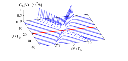
Figure 6: (color online) The differential Andreev conductance $G_{A}(V)$ versus the Coulomb potential $U$ and bias $V$ obtained in the superconducting atomic limit $\Delta\gg\Gamma_{S}$ for $T=0$, $\Gamma_{S}/\Gamma_{N}=20$ in absence of the boson mode $g=0$. The thick (red) line indicates the QPT at $U=\Gamma_{S}$.

In absence of the boson field (i.e for $\lambda\!=\!0$) the exact solution of such problem has been discussed by a number of authors (e.g. see the references cited in Baranski_2013 ). The effective quasiparticle energies are given by $\pm U/2\pm E_{d}$, where $E_{d}=\sqrt{(\varepsilon+U/2)^{2}+(\Gamma_{S}/2)^{2}}$. In the realistic situations only two branches $\pm\left(U/2-E_{d}\right)$ appear in the subgap regime, whereas the other high energy states $\pm\left(U/2+E_{d}\right)$ overlap with a continuum beyond the gap. The quantum phase transition (QPT) from the singlet $u\left|0\right>+v\left|\uparrow\downarrow\right>$ to doublet $\left|\sigma\right>$ configuration occurs at $U/2=E_{d}$ Bauer-08 . In order to estimate quantitatively the Andreev conductance we use the off-diagonal Green’s function ${\mbox{\boldmath{$f$}}}(\omega)$ Bauer-08 ; Baranski_2013 , restricting to its subgap part

$${\mbox{\boldmath{$f$}}}_{sub}(\omega)\simeq\frac{\alpha\;uv}{\omega\!+\!\frac{i\Gamma_{N}}{2}-\left(\frac{U}{2}\!-\!E_{d}\right)}-\frac{\alpha\;uv}{\omega\!+\!\frac{i\Gamma_{N}}{2}+\left(\frac{U}{2}\!-\!E_{d}\right)}$$

(33)

with the usual BCS coefficient $uv=\Gamma_{S}/4E_{d}$ and the spectral weight $\alpha=\left[\mbox{\rm exp}\left({\frac{U}{2k_{B}T}}\right)+\mbox{\rm exp}\left(\frac{E_{d}}{k_{B}T}\right)\right]/{\cal{Z}}$, where ${\cal{Z}}=2\;\mbox{\rm exp}\left({\frac{U}{2k_{B}T}}\right)+\mbox{\rm exp}\left(\frac{-E_{d}}{k_{B}T}\right)+\mbox{\rm exp}\left(\frac{E_{d}}{k_{B}T}\right)$. The missing part of spectral weight $1-\alpha$ belongs to the high-energy states (outside the gap). At zero temperature this subgap weight changes abruptly from $\alpha=1$ (in the singlet state when $U/2<E_{d}$) to $\alpha=0.5$ (in the doublet state when $U/2>E_{d}$).

In figure 6 we plot the Andreev conductance obtained for the half-filled quantum dot $\varepsilon=-U/2$ (QPT occurs then at $U=\Gamma_{S}$). We notice the subgap conductance enhancements around $|eV|=U/2-E_{d}$. Yet, exactly at the QPT, both the singlet and doublet contributions cancel each other. Formally, this is due to the odd (asymmetric) structure of the Green’s function (33).

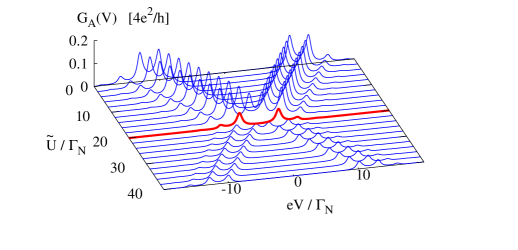
Figure 7: (color online) The subgap Andreev conductance $G_{A}(V)$ as a function of the Coulomb potential $\tilde{U}$ and voltage $V$ obtained for $g=1$, $\omega_{0}/\Gamma_{N}=10$ and the same model parameters as in figure 6.

The superconducting atomic limit solution can be generalized onto $g\neq 0$ case in a straightforward way. The unitary transformation (2) implies $\varepsilon\rightarrow\tilde{\varepsilon}$, $U\rightarrow\tilde{U}$ and following the steps (10-29) we can determine the off-diagonal Green’s function. At zero temperature, we find

$${\mbox{\boldmath{$F$}}}_{sub}(\omega) \simeq \alpha\;uv\;\sum_{l=0}^{\infty}\left\{\frac{e^{-g}\;(-g)^{l}\;/l!}{\omega\!+\!\frac{i\Gamma_{N}}{2}-\left(\frac{\tilde{U}}{2}\!-\!E_{d}\right)\!+\!s\;l\omega_{0}}\right.$$ (34)

$$- \left.\frac{e^{-g}\;(-g)^{l}\;/l!}{\omega\!+\!\frac{i\Gamma_{N}}{2}+\left(\frac{\tilde{U}}{2}\!-\!E_{d}\right)\!-\!s\;l\omega_{0}}\right\}$$

with $s\equiv\mbox{\rm sign}(\frac{\tilde{U}}{2}-E_{d})$.

Figure 7 shows the Andreev conductance obtained for the half-filled quantum dot using $g=1$, $\omega_{0}/\Gamma_{N}=10$, $\Gamma_{S}/\Gamma_{N}=20$, $T=0$. The bosonic side-peaks give rise to additional subgap branches, similar to what has been reported for the spectral function Zitko_2012 . Right at the QPT, the zero-bias conductance again vanishes $G(0)\rightarrow 0$ and we observe only the higher order maxima at $|eV|=l\omega_{0}$ (with $l\geq 1$). Away from the QPT, the Andreev conductance shows the usual maxima at $|eV|=|\tilde{U}/2-E_{d}|+l\omega_{0}$ whose spectral weights depend on $\tilde{U}$ and $l$.

VI Summary

We have investigated the subgap spectrum and transport properties of the quantum dot coupled between the metallic and superconducting electrodes in presence of the external boson mode $\omega_{0}$. We have found that the induced Andreev states eventually cross each upon varying the gate potential (through $\varepsilon$) or due to the correlations (via quantum phase transition from the singlet to doublet configurations). We have explored their signatures in the measurable charge transport. The tunneling conductance of such multilevel ’molecule’ shows a series of characteristic enhancements, dependent on: the gate voltage with frequency $\omega_{0}/2$ (which can be deduced from Eqn. 30), the bias $V$ applied between external leads (Fig. 5), and the correlations (Fig. 7). External boson reservoir can thus substantially affect the anomalous Andreev current and it can be probed experimentally using the low-energy vibrational modes or the slowly-varying ac fields Platero_Aguado_2004 .

References

- (1) G. Platero and R. Aguado, Phys. Rep. 395, 1 (2004).
- (2) M. Galperin, M.A. Ratner, and A. Nitzan, J. Phys.: Condens. Matter 19, 103201 (2007).
- (3) J. Koch and F. von Oppen, Phys. Rev. Lett. 94, 206804 (2005); J. Koch, F. von Oppen, and A.V. Andreev, Phys. Rev. B 74, 2054368 (2006).
- (4) J. Fransson, Non-Equilibrium Nano-Physics: A Many-Body Approach, Lecture Notes in Physics 809 (Springer, Dordrecht 2010).
- (5) S. Sapmaz, P. Jarillo-Herrero, Ya.M. Blanter, C. Dekker, and H.S.J. van der Zant, Phys. Rev. Lett. 96, 026801 (2006).
- (6) R. Leturcq, C. Stampfer, K. Inderbitzin, L. Durrer, C. Hierold, E. Mariani, M.G. Schultz, F. von Oppen F, and K. Ensslin, Nature Phys. 5, 327 (2009).
- (7) J.M. Beebe, B.S. Kim, J.W. Gadzuk, C.D. Frisbie, and J.G. Kushmerick, Phys. Rev. Lett. 97, 026801 (2006).
- (8) A.N. Pasupathy, J. Park, C. Chang, A.V. Soldatov, S. Lebedkin, R.C. Bialczak, J.E. Grose, L.A.K. Donev, J.P. Sethna, D.C. Ralph, and P.L. McEuen, NanoLetters 5, 203 (2005).
- (9) A. Zazunov, R. Egger, C. Mora, and T. Martin, Phys. Rev. B 73, 214501 (2006).
- (10) J. Fransson, A.V. Balatsky, and J.-X. Zhu, Phys. Rev. B 81, 155440 (2010).
- (11) B.H. Wu, J.C. Cao, and C. Timm, Phys. Rev. B 86, 035406 (2012).
- (12) S.Y. Cho, K. Kang, and C.-M. Ryu, Phys. Rev. B 60, 16874 (1999).
- (13) P. Zhang and Y.-X. Li, J. Phys.: Condens. Matter 21, 095602 (2009);
- (14) L. Bai, Z.-Z. Zhang, and J. Jiang, Phys. Lett. A 375, 661 (2011).
- (15) D. Golež, J. Bonča, and R. Žitko, Phys. Rev. B 86, 085142 (2012).
- (16) S.N. Zhang, W. Pei, T.F. Fang, and Q.F. Sun, Phys. Rev. B 86, 104513 (2012).
- (17) K. Bocian and W. Rudziński, Acta Phys. Polon. A 126, 374 (2014).
- (18) H.-Y. Song and S.-P. Zhou, Phys. Lett. A 372, 6773 (2008).
- (19) K.F. Albrecht, H. Soller, L. Mühlbacher, and A. Komnik, Physica E 54, 15 (2013).
- (20) Q. Wang, H. Xie, H. Jiao, and Y.-H. Nie, Europhys. Lett. 101, 47008 (2013).
- (21) A.V. Balatsky, I. Vekhter, and J.-X. Zhu, Rev. Mod. Phys. 78, 373 (2006).
- (22) I.G. Lang and Y.A. Firsov, Sov. Phys. JETP 16, 1301 (1963).
- (23) G.D. Mahan, Many-Particle Physics (Plenum Press, New York, 1990).
- (24) Q.-F. Sun, J. Wang, and T.-H. Lin, Phys. Rev. B 59, 3831 (1999); Q.-F. Sun, H. Guo, and T.-H. Lin, Phys. Rev. Lett. 87, 176601 (2001); M. Krawiec and K.I. Wysokiński, Supercond. Sci. Technol. 17, 103 (2004).
- (25) R.S. Deacon, Y. Tanaka, A. Oiwa, R. Sakano, K. Yoshida, K. Shibata, K. Hirakawa, and S. Tarucha, Phys. Rev. Lett. 104, 076805 (2010); R.S. Deacon, Y. Tanaka, A. Oiwa, R. Sakano, K. Yoshida, K. Shibata, K. Hirakawa, and S. Tarucha, Phys. Rev. B 81, 121308(R) (2010).
- (26) J.D. Pillet, P. Joyez, R. Žitko, and F.M. Goffman, Phys. Rev. B 88, 045101 (2013).
- (27) J. Schindele, A. Baumgartner, R. Maurand, M. Weiss, and C. Schönenberger, Phys. Rev. B 89, 045422 (2014).
- (28) E.J.H. Lee, X. Jiang, R. Aguado, G. Katsaros, C.M. Lieber, and S. De Franceschi, Phys. Rev. Lett. 109, 186802 (2012).
- (29) E.J.H. Lee, X. Jiang, M. Houzet, R. Aguado, Ch.M. Lieber, S. De Franceschi, Nature Nanotechnology 9, 79 (2014).
- (30) T. Domański and A. Donabidowicz, Phys. Rev. B 78, 073105 (2008); T. Domański, A. Donabidowicz, and K.I. Wysokiński, Phys. Rev. B 78, 144515 (2008); Phys. Rev. B 76, 104514 (2007).
- (31) V. Koerting, B.M. Andersen, K. Flensberg, and J. Paaske, Phys. Rev. B 82, 245108 (2010);
- (32) A. Martín-Rodero and A. Levy Yeyati, Adv. Phys. 60, 899 (2011); A. Martín-Rodero and A. Levy Yeyati, J. Phys.: Condens. Matter 24, 385303 (2012).
- (33) Y. Yamada, Y. Tanaka, and N. Kawakami, Phys. Rev. B 84, 075484 (2011); A. Oguri, Y. Tanaka, and J. Bauer, Phys. Rev. B 87, 075432 (2013).
- (34) R. Žitko, J.S. Lim, R. López, and R. Aguado, Phys. Rev. B 91, 045441 (2015).
- (35) J. Bauer, A. Oguri, and A.C. Hewson, J. Phys.: Condens. Matter 19, 486211 (2008).
- (36) J. Barański and T. Domański, J. Phys.: Condens. Matter 25, 435305 (2013).