EUROPEAN ORGANIZATION FOR NUCLEAR RESEARCH (CERN)

​​​ CERN-PH-EP-2015-072 LHCb-PAPER-2015-010 June 12, 2015

Observation of the decay $\overline{B}_{s}^{0}\rightarrow\psi(2S)K^{+}\pi^{-}$

The LHCb collaboration

The decay $\overline{B}_{s}^{0}\rightarrow\psi(2S)K^{+}\pi^{-}$ is observed using a data set corresponding to an integrated luminosity of $3.0\mbox{\,fb}^{-1}$ collected by the LHCb experiment in $pp$ collisions at centre-of-mass energies of 7 and 8 TeV. The branching fraction relative to the ${{B}^{0}}\rightarrow\psi(2S)K^{+}\pi^{-}$ decay mode is measured to be

$$\frac{{\cal B}(\overline{B}^{0}_{s}\rightarrow\psi(2S)K^{+}\pi^{-})}{{\cal B}(B^{0}\rightarrow\psi(2S)K^{+}\pi^{-})}=5.38\pm 0.36\mathrm{\,(stat)}\pm 0.22\mathrm{\,(syst)}\pm 0.31\,(f_{s}/f_{d})\,\%,$$

where $f_{s}/f_{d}$ indicates the uncertainty due to the ratio of probabilities for a $b$ quark to hadronise into a ${{B}^{0}_{s}}$ or ${{B}^{0}}$ meson. Using an amplitude analysis, the fraction of decays proceeding via an intermediate $K^{*}(892)^{0}$ meson is measured to be $0.645\pm 0.049\mathrm{\,(stat)}\pm 0.049\mathrm{\,(syst)}$ and its longitudinal polarisation fraction is $0.524\pm 0.056\mathrm{\,(stat)}\pm 0.029\mathrm{\,(syst)}$. The relative branching fraction for this component is determined to be

$$\frac{{\cal B}(\overline{B}^{0}_{s}\rightarrow\psi(2S)K^{*}(892)^{0})}{{\cal B}(B^{0}\rightarrow\psi(2S)K^{*}(892)^{0})}=5.58\pm 0.57\mathrm{\,(stat)}\pm 0.40\mathrm{\,(syst)}\pm 0.32\,(f_{s}/f_{d})\,\%.$$

In addition, the mass splitting between the ${{B}^{0}_{s}}$ and ${{B}^{0}}$ mesons is measured as

$$M(B^{0}_{s})-M(B^{0})=87.45\pm 0.44\mathrm{\,(stat)}\pm 0.09\mathrm{\,(syst)}{\mathrm{\,Me\kern-1.00006ptV\!/}c^{2}}.$$

Published in Phys. Lett. B

© CERN on behalf of the LHCb collaboration, license CC-BY-4.0.

 

1 Introduction

The large data set collected by the LHCb experiment has allowed precision measurements of time-dependent $C\!P$ violation in the ${{B}^{0}_{s}}\rightarrow J/\psi\phi$ and ${{B}^{0}_{s}}\rightarrow J/\psi f_{0}(980)$ decay modes [1, 2]. The results are interpreted assuming that these decays are dominated by colour-suppressed tree-level amplitudes (Fig. 1). Higher-order penguin amplitudes, which are difficult to calculate in QCD, also contribute (Fig. 1). Reference [3] suggests that the size of contributions from these processes can be determined by studying decay modes such as ${{\kern 1.79993pt\overline{\kern-1.79993ptB}{}}{}^{0}_{s}}\rightarrow J/\psi K^{*}(892)^{0}$ where they dominate. The ${{\kern 1.79993pt\overline{\kern-1.79993ptB}{}}{}^{0}_{s}}\rightarrow J/\psi K^{*}(892)^{0}$ decay mode was first observed by the CDF collaboration [4] and subsequently studied in detail by the LHCb collaboration [5].

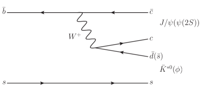
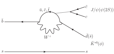
Figure 1: Tree (left) and penguin (right) topologies contributing to the ${{B}^{0}_{({s})}}\rightarrow\psi V$ decays where $\psi=J/\psi,\psi(2S)$ and $V=\phi,K^{*}(892)^{0}$.

Recently, interest in $b$-hadron decays to final states containing charmonia has been generated by the observation of the $Z(4430)^{-}\rightarrow\psi(2S)\pi^{-}$ state in the ${{B}^{0}}\rightarrow\psi(2S)K^{+}\pi^{-}$ decay chain by the Belle [6, 7, 8] and LHCb collaborations [9]. As this state is charged and has a minimal quark content of ${c}{\overline{c}}{d}{\overline{u}}$, it is interpreted as evidence for the existence of non-$q\overline{q}$ mesons [10]. Evidence for similar exotic structures in ${{B}^{0}}\rightarrow\chi_{c1,c2}K^{+}\pi^{-}$ and ${{B}^{0}}\rightarrow J/\psi K^{+}\pi^{-}$decays has been reported by the Belle collaboration[11, 12]. If these structures correspond to real particles they should be visible in other decay modes.

This letter reports the first observation of the decay $\overline{B}_{s}^{0}\rightarrow\psi(2S)K^{+}\pi^{-}$ and presents measurements of the inclusive branching fraction and the fraction of decays that proceed via an intermediate ${{K}^{*}}(892)^{0}$ resonance, as determined from an amplitude analysis of the final state. The amplitude analysis also allows the determination of the longitudinal polarisation fraction of the ${{K}^{*}}(892)^{0}$ meson. Additionally a measurement of the mass difference between ${B}^{0}_{s}$ and ${B}^{0}$ mesons is reported that improves the current knowledge of this observable.

2 Detector and simulation

The LHCb detector [13, 14] is a single-arm forward spectrometer covering the pseudorapidity range $2<\eta<5$, designed for the study of particles containing $b$ or $c$ quarks. The detector includes a high-precision tracking system consisting of a silicon-strip vertex detector surrounding the $pp$ interaction region, a large-area silicon-strip detector located upstream of a dipole magnet with a bending power of about $4{\rm\,Tm}$, and three stations of silicon-strip detectors and straw drift tubes [15] placed downstream of the magnet. The tracking system provides a measurement of momentum, $p$, of charged particles with a relative uncertainty that varies from 0.5% at low momentum to 1.0% at 200${\mathrm{\,Ge\kern-1.00006ptV\!/}c}$. The minimum distance of a track to a primary vertex, the impact parameter, is measured with a resolution of $(15+29/\mbox{$p_{\rm T}$}){\,\upmu\rm m}$, where $p_{\rm T}$ is the component of the momentum transverse to the beam, in ${\mathrm{\,Ge\kern-1.00006ptV\!/}c}$. Large samples of $B^{+}\rightarrow{{J\mskip-3.0mu/\mskip-2.0mu\psi\mskip 2.0mu}}K^{+}$ and ${{J\mskip-3.0mu/\mskip-2.0mu\psi\mskip 2.0mu}}\rightarrow{\mu^{+}}{\mu^{-}}$ decays, collected concurrently with the data set used here, were used to calibrate the momentum scale of the spectrometer to a precision of $0.03\,\%$ [16].

Different types of charged hadrons are distinguished using information from two ring-imaging Cherenkov detectors [17]. Photons, electrons and hadrons are identified by a calorimeter system consisting of scintillating-pad and preshower detectors, an electromagnetic calorimeter and a hadronic calorimeter. Muons are identified by a system composed of alternating layers of iron and multiwire proportional chambers [18]. The online event selection is performed by a trigger [19], which consists of a hardware stage, based on information from the calorimeter and muon systems, followed by a software stage, which applies a full event reconstruction. In this analysis candidates are first required to pass the hardware trigger, which selects muons and dimuon pairs based on the transverse momentum. At the subsequent software stage, events are triggered by a $\psi(2S)\rightarrow\mu^{+}\mu^{-}$ candidate where the $\psi(2S)$ is required to be consistent with coming from the decay of a ${b}$ hadron by either using impact parameter requirements on daughter tracks or detachment of the $\psi(2S)$ candidate from the primary vertex.

The analysis is performed using data corresponding to an integrated luminosity of 1.0 fb^-1 collected in $pp$ collisions at a centre-of-mass energy of 7 TeV and 2.0 fb^-1 collected at 8 TeV. In the simulation, $pp$ collisions are generated using Pythia [20, *Sjostrand:2007gs] with a specific LHCb configuration [22]. Decays of hadronic particles are described by EvtGen [23], in which final state radiation is generated using Photos [24]. The interaction of the generated particles with the detector and its response are implemented using the Geant4 toolkit [25, *Agostinelli:2002hh] as described in Ref. [27].

3 Event selection

The selection of candidates is divided into two parts. First, a loose selection is performed that retains the majority of signal events whilst reducing the background substantially. After this the ${{B}^{0}}\rightarrow\psi(2S)K^{+}\pi^{-}$ peak is clearly visible. Subsequently, a multivariate method is used to further improve the signal-to-background ratio and to allow the observation of the ${{\kern 1.79993pt\overline{\kern-1.79993ptB}{}}{}^{0}_{s}}\rightarrow\psi(2S)K^{+}\pi^{-}$ decay.

The selection starts by reconstructing the dimuon decay of the $\psi(2S)$ meson. Pairs of oppositely charged particles identified as muons with $\mbox{$p_{\rm T}$}>550{\mathrm{\,Me\kern-1.00006ptV\!/}c}$ are combined to form $\psi(2S)$ candidates. The invariant mass of the dimuon pair is required to be within $60{\mathrm{\,Me\kern-1.00006ptV\!/}c^{2}}$ of the known $\psi(2S)$ mass [28]. To form ${{B}^{0}_{({s})}}$ candidates, the selected $\psi(2S)$ mesons are combined with oppositely charged kaon and pion candidates. Tracks that do not correspond to actual trajectories of charged particles are suppressed by requiring that they have $\mbox{$p_{\rm T}$}>250{\mathrm{\,Me\kern-1.00006ptV\!/}c}$ and by selecting on the output of a neural network trained to discriminate between these and genuine tracks associated to particles. Combinatorial background from hadrons originating in the primary vertex (PV) is suppressed by requiring that both hadrons are significantly displaced from any PV. Well-identified hadrons are selected using the information provided by the Cherenkov detectors. This is combined with kinematic information using a neural network to provide a probability that a particle is a kaon ($\mathcal{P}^{K}$), pion ($\mathcal{P}^{\pi}$) or proton ($\mathcal{P}^{p}$). It is required that $\mathcal{P}^{K}$ is larger than 0.1 for the $K^{+}$ candidate and that $\mathcal{P}^{\pi}$ is larger than 0.2 for the $\pi^{-}$ candidate.

A kinematical vertex fit is applied to the ${{B}^{0}_{({s})}}$ candidates [29]. To improve the invariant mass resolution, the fit is performed with the requirement that the ${{B}^{0}_{({s})}}$ candidate points to the PV and the $\psi(2S)$ is mass constrained to the known value [28]. A good quality of the vertex fit $\chi^{2}$, $\chi^{2}_{\mathrm{DTF}}$, is required. To ensure good separation between the ${{B}^{0}}$ and ${{B}^{0}_{s}}$ signals, the uncertainty on the reconstructed mass returned by the fit must be less than 11${\mathrm{\,Me\kern-1.00006ptV\!/}c^{2}}$. Combinatorial background from particles produced in the primary vertex is further reduced by requiring the decay time of the ${{B}^{0}_{({s})}}$ meson to exceed $0.3{\rm\,ps}$.

Four criteria are applied to reduce background from specific ${b}$-hadron decay modes. First, the candidate is rejected if the invariant mass of the hadron pair calculated assuming that both particles are kaons is within $10{\mathrm{\,Me\kern-1.00006ptV\!/}c^{2}}$ of the known $\phi$ meson mass [28], suppressing ${{B}^{0}_{s}}\rightarrow\psi(2S)\phi$ decays where one of the kaons is misidentified as a pion. Second, to suppress $B^{0}\rightarrow\psi(2S)\pi^{+}\pi^{-}$ events where one of the pions is incorrectly identified as a kaon, it is required that $\mathcal{P}^{K}>\mathcal{P}^{\pi}$ for the kaon candidate. This rejects $80\,\%$ of the background from this source whilst retaining $90\,\%$ of ${{B}^{0}_{({s})}}$ signal candidates. Third, to suppress background from ${{\mathchar 28931\relax}^{0}_{b}}\rightarrow\psi(2S){p}\pi^{-}$ decays where the proton is misidentifed as a kaon, candidates with $\mathcal{P}^{p}>0.3$ and an invariant mass within $15{\mathrm{\,Me\kern-1.00006ptV\!/}c^{2}}$ of the known ${{\mathchar 28931\relax}^{0}_{b}}$ mass [28] are discarded. Finally, to reduce background from a $B^{+}\rightarrow\psi(2S)K^{+}$ decay combined with a random pion, candidates where the reconstructed $\psi(2S)K^{+}$ invariant mass is within $16{\mathrm{\,Me\kern-1.00006ptV\!/}c^{2}}$ of the known $B^{+}$ mass [28] are rejected. Background from the decay ${{\mathchar 28931\relax}^{0}_{b}}\rightarrow\psi(2S){p}K^{-}$ with misidentified hadrons does not peak at the ${{B}^{0}_{s}}$ mass and is modelled in the fit.

To further improve the signal-to-background ratio, a multivariate analysis based on a neural network is used. This is trained using simulated ${{B}^{0}}$ signal events together with candidates from data with a mass between $5500$ and $5600{\mathrm{\,Me\kern-1.00006ptV\!/}c^{2}}$ that are not used for subsequent analysis. Eight variables that give good separation between signal and background are used: the number of clusters in the large-area silicon tracker upstream of the magnet, $\mathcal{P}^{K}$ for the kaon candidate, $\mathcal{P}^{\pi}$ for the pion candidate, the transverse momentum of the ${{B}^{0}_{({s})}}$, the minimum impact parameter to any primary vertex for each of the two hadrons, $\chi^{2}_{\mathrm{DTF}}$ and the flight distance in the laboratory frame of the ${{B}^{0}_{({s})}}$ candidate divided by its uncertainty. The ratio $N_{\rm S}/\sqrt{N_{\rm S}+N_{\rm B}}$ is used as a figure of merit, where $N_{\rm S}\ (N_{\rm B})$ is the number of signal (background) events determined from the invariant mass fit (see Sect. 4). The maximum value of this ratio is found for a threshold on the neural network output that rejects $98\%$ of the background and retains $81\%$ of the signal for subsequent analysis.

4 Invariant mass fit

A maximum likelihood fit is made to the unbinned $\psi(2S)K^{+}\pi^{-}$ invariant mass distribution, $m(\psi(2S){{K}^{+}}\pi^{-})$, to extract the ${{B}^{0}}$ and ${{B}^{0}_{s}}$ signal yields. The ${{B}^{0}}$ signal component is modelled by the sum of two Crystal Ball functions [30] with common tail parameters and an additional Gaussian component, all with a common mean. All parameters are fixed to values determined from the simulation apart from the common mean and an overall resolution scale factor. The simulation is tuned to match the invariant mass resolution seen in data for the ${{B}^{+}}\rightarrow J/\psi K^{+}$ and ${{B}^{0}}\rightarrow{{J\mskip-3.0mu/\mskip-2.0mu\psi\mskip 2.0mu}}{{K}^{+}}\pi^{-}$ decay modes. Consequently, the resolution scale factor is consistent with unity in the fit to data. The ${{B}^{0}_{s}}$ component is modelled with the same function, with the mean value of the ${{B}^{0}_{s}}$ meson mass left free in the fit. The resolution parameters in this case are multiplied by a factor of 1.06, determined from simulation, which accounts for the additional energy release in this decay.

The dominant background is combinatorial and modelled by an exponential function. A significant component from ${{B}^{0}_{s}}\rightarrow\psi(2S)\phi$ decays is visible at lower masses than the ${{B}^{0}}$ peak. This is modelled in the fit by a bifurcated Gaussian function where the shape parameters are constrained to the values obtained in the simulation and the yield constrained to the value determined in data under the hypothesis that both hadrons are kaons. Additional small components from $B^{0}_{(s)}\rightarrow\psi(2S)\pi^{+}\pi^{-}$ and ${{\mathchar 28931\relax}^{0}_{b}}\rightarrow\psi(2S){p}K^{-}$ decays are modelled by bifurcated Gaussian functions. The shapes of these components are fixed using the simulation and the yields are determined by normalising the simulation samples to the number of candidates for each modes found in data using dedicated selections. Contributions from partially reconstructed decays are accounted for in the combinatorial background. In total, the fit has ten free parameters. Variations of this fit model are considered as systematic uncertainties.

Figure 2 shows the invariant mass distribution observed in the data together with the result of a fit to the model described above. Binning the data, a $\chi^{2}$-probability of 0.30 is found. The moderate mismodelling of the ${B}^{0}$ peak is accounted for in the systematic uncertainties. The fit determines that there are $329\pm 22$ ${{B}^{0}_{s}}$ decays and $24207\pm 160$ ${{B}^{0}}$ decays. The ${{\kern 1.79993pt\overline{\kern-1.79993ptB}{}}{}^{0}_{s}}\rightarrow\psi(2S)K^{+}\pi^{-}$ mode is observed with high significance.

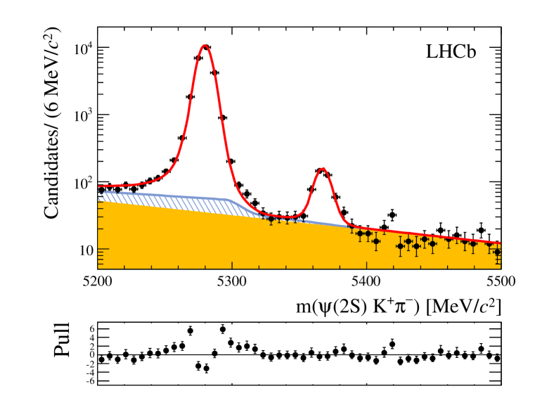
Figure 2: Invariant mass distribution for selected $\psi(2S)K^{+}\pi^{-}$ candidates in the data. A fit to the model described in the text is superimposed. The full fit model is shown by the solid (red) line, the combinatorial background by the solid (yellow) and the sum of background from the exclusive $b\rightarrow\psi(2S)X$ modes considered in the text by the shaded (blue) area. The maximum of the $y$-scale is restricted so as to be able to see more clearly the ${{\kern 1.61993pt\overline{\kern-1.61993ptB}{}}{}^{0}_{s}}\rightarrow\psi(2S)K^{+}\pi^{-}$ signal. The lower plot shows the differences between the fit and measured values divided by the corresponding uncertainty of the measured value, the so-called pull distribution.

The precision of the momentum scale calibration of $0.03\%$ translates to an uncertainty on the ${B}^{0}$ and ${B}^{0}_{s}$ meson masses of $0.3{\mathrm{\,Me\kern-1.00006ptV\!/}c^{2}}$. Therefore, it is chosen to quote only the mass difference in which this uncertainty largely cancels,

$$M({{B}^{0}_{s}})-M({{B}^{0}})=87.45\pm 0.44\mathrm{\,(stat)}\pm 0.09\mathrm{\,(syst)}{\mathrm{\,Me\kern-1.00006ptV\!/}c^{2}}.$$

This procedure has been checked using the simulation, which gives the input mass difference with a bias of $0.05{\mathrm{\,Me\kern-1.00006ptV\!/}c^{2}}$ that is assigned as a systematic uncertainty. Further systematic uncertainties arise from the momentum scale and mass fit model. Varying the momentum scale by $0.03\%$ leads to an uncertainty of $0.04{\mathrm{\,Me\kern-1.00006ptV\!/}c^{2}}$. The effect of the fit model is evaluated by considering several variations: the relative fraction of the two Crystal Ball functions is left free; the slope of the combinatorial background is constrained using candidates where the kaon and pion have the same charge; the Gaussian constraints on the background from the ${{B}^{0}_{s}}\rightarrow\psi(2S)\phi$ mode are removed; and the tail parameters of the Crystal Ball functions are left free. The largest variation in the mass splitting is $0.06\,{\mathrm{\,Me\kern-1.00006ptV\!/}c^{2}}$. The total systematic uncertainty is given by summing the individual components in quadrature.

5 Amplitude analysis

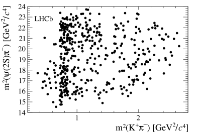
Figure 3: Dalitz plot for the selected ${{\kern 1.61993pt\overline{\kern-1.61993ptB}{}}{}^{0}_{s}}\rightarrow\psi(2S){{K}^{+}}\pi^{-}$ candidates in the signal window $m(\psi(2S){{K}^{+}}\pi^{-})\in[5350,5380]{\mathrm{\,Me\kern-0.90005ptV\!/}c^{2}}$.

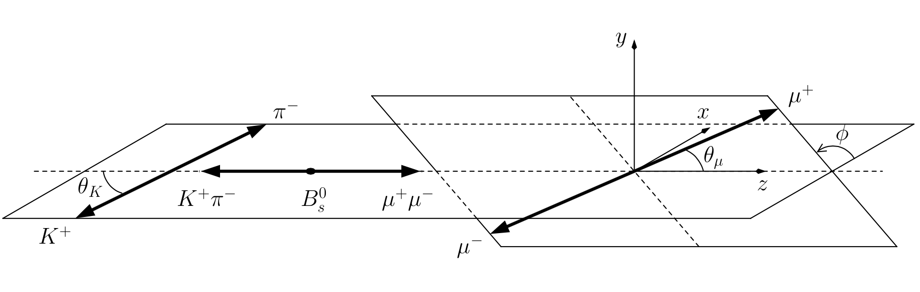
Figure 4: Definition of the helicity angles.

Figure 3 shows the Dalitz plot of the selected ${{\kern 1.79993pt\overline{\kern-1.79993ptB}{}}{}^{0}_{s}}\rightarrow\psi(2S){{K}^{+}}\pi^{-}$ candidates in the signal range, $m(\psi(2S){{K}^{+}}\pi^{-})\in[5350,5380]{\mathrm{\,Me\kern-1.00006ptV\!/}c^{2}}$. There is a clear enhancement around the known ${{K}^{*}}(892)^{0}$ mass [28] and no other significant enhancements elsewhere. To determine the fraction of decays that proceed via the ${{K}^{*}}(892)^{0}$ resonance, an amplitude analysis is performed, similar to that used in Ref. [9] for the analysis of the ${{B}^{0}}\rightarrow\psi(2S)K^{+}\pi^{-}$ mode. The final-state particles are described using three angles $\Omega\equiv(\cos\theta_{K},\cos\theta_{\mu},\phi)$ in the helicity basis, defined in Fig. 4, and the invariant $K^{+}\pi^{-}$ mass, $m_{K\pi}\equiv m({{K}^{+}}\pi^{-})$. The total amplitude is $S(m_{K\pi},\Omega)\varepsilon(m_{K\pi},\Omega)+B(m_{K\pi},\Omega)$, where $S(m_{K\pi},\Omega)$ represents the coherent sum over the helicity amplitudes for each considered ${{K}^{+}}\pi^{-}$ resonance or non-resonant component. The detection efficiency, $\varepsilon(m_{K\pi},\cos\theta_{K},\cos\theta_{\mu},\phi)$, is evaluated using simulation and parameterised using a combination of Legendre polynomials and spherical harmonic moments, given by

$$\small\varepsilon(m_{K\pi},\cos\theta_{K},\cos\theta_{\mu},\phi)=\sum_{a,b,c,d}c^{abcd}P_{a}(\cos\theta_{K})Y_{bc}(\cos\theta_{\mu},\phi)P_{d}\left(\frac{2(m_{K\pi}-m_{K\pi}^{\rm min})}{m_{K\pi}^{\rm max}-m_{K\pi}^{\rm min}}-1\right),$$ (1)

where $m_{K\pi}^{\rm min(max)}$ is the minimum (maximum) value allowed for $m_{K\pi}$ in the available phase space of the decay. The coefficients of the efficiency parameterisation are computed by summing over the $N_{\rm MC}$ events simulated uniformly in the phase-space as

$$c^{abcd}=\frac{1}{N_{\rm MC}}\sum_{i}^{N_{\rm MC}}\frac{2a+1}{2}\frac{2d+1}{2}P_{a}({\cos\theta_{K}}_{i})Y_{bc}({\cos\theta_{\mu}}_{i},{\phi}_{i})P_{d}\left(\frac{2({m_{K\pi}}_{i}-m_{K\pi}^{\rm min})}{m_{K\pi}^{\rm max}-m_{K\pi}^{\rm min}}-1\right)\frac{C}{g_{i}},$$ (2)

where $g_{i}=p_{i}q_{i}$, with $p_{i}\,(q_{i})$ being the momentum of the $K^{+}\pi^{-}$ system ($K^{+}$ meson) in the $B^{0}\ (K^{+}\pi^{-})$ rest frame and $C$ is a normalising constant with units ${\rm GeV}^{2}/c^{2}$. This approach provides a description of the multidimensional correlations without assuming factorisation. In practice, the sum is over a finite number of moments ($a\leq 2$, $b\leq 2$, $c\leq 2$ and $d\leq 2$) and only coefficients with a statistical significance larger than five standard deviations from zero are retained. The one-dimensional projections of the parameterised efficiency are shown in Fig. 5, superimposed on the simulated event distributions.

\begin{overpic}[width=432.48048pt]{Fig5.pdf} \put(10.0,60.0){(a)} \put(60.0,60.0){(b)} \put(10.0,27.0){(c)} \put(60.0,27.0){(d)} \end{overpic}

Figure 5: Distributions of (a) $\cos\theta_{\mu}$, (b) $\phi$, (c) $\cos\theta_{K}$ and (d) $m({{K}^{+}}\pi^{-})$ of simulated $B^{0}_{s}\rightarrow\psi(2S){{K}^{+}}\pi^{-}$ decays in a phase space configuration (black points) with the parameterisation of the efficiency overlaid (blue lines).

The background probability density function, $B(m_{K\pi},\Omega)$, is determined using a similar method as for the efficiency parameterisation. In this case the sum in Eq. (2) is over the selected events with $m(\psi(2S){{K}^{+}}\pi^{-})>5390{\mathrm{\,Me\kern-1.00006ptV\!/}c^{2}}$ and $g_{i}\equiv 1$. Only moments with $a\leq 2$, $b=0$, $c=0$ and $d\leq 2$ and a statistical significance larger than five standard deviations from zero are retained. The one-dimensional projections of the parameterised background distribution are shown in Fig. 6, superimposed on the sideband data. As a consistency check, the $(m_{K\pi},\Omega)$ distributions for events with $m(\psi(2S){{K}^{+}}\pi^{-})>5390{\mathrm{\,Me\kern-1.00006ptV\!/}c^{2}}$ are found to be compatible with the same distributions obtained from a like-sign ($\psi(2S)K^{\pm}\pi^{\pm}$) sample.

\begin{overpic}[width=432.48048pt]{Fig6.pdf} \put(10.0,60.0){(a)} \put(60.0,60.0){(b)} \put(10.0,27.0){(c)} \put(60.0,27.0){(d)} \end{overpic}

Figure 6: Distributions of (a) $\cos\theta_{\mu}$, (b) $\phi$, (c) $\cos\theta_{K}$ and (d) $m({{K}^{+}}\pi^{-})$ of $B^{0}_{(s)}\rightarrow\psi(2S){{K}^{+}}\pi^{-}$ candidates with $m(\psi(2S){{K}^{+}}\pi^{-})>5390{\mathrm{\,Me\kern-0.90005ptV\!/}c^{2}}$ (black points), with the parameterisation of the background distribution overlaid (blue lines).

The default amplitude model is constructed using contributions from the ${{K}^{*}}(892)^{0}$ resonance and a ${{K}^{+}}\pi^{-}$ S-wave modelled using the LASS parameterisation [31]. The magnitudes and phases of all components are measured relative to those of the zero helicity state of the ${{K}^{*}}(892)^{0}$ meson and the masses and widths of the resonances are fixed to their known values [28]. The remaining eight free parameters are determined using a maximum likelihood fit of the amplitude to the data in the signal window. The background fraction is fixed to $0.28$, as determined from the fit described in Sect. 4. The fit fraction for any resonance $R$ is defined in the full phase space, as $f_{R}=\int S_{R}\,{\rm d}m_{K\pi}{\rm d}\Omega\,/\int S\,{\rm d}m_{K\pi}{\rm d}\Omega$, where $S_{R}$ is the signal amplitude with all amplitude terms set to zero except those for $R$. The fractions of each component determined by the fit are $f_{K^{*}(892)^{0}}=0.645\pm 0.049$, and $f_{\rm S-wave}=0.339\pm 0.052$, where the uncertainty is statistical only. The fractions do not sum to unity due to interference between the different components. Variations of the S-wave description and default mixture of ${{K}^{+}}\pi^{-}$ resonances, including the introduction of the spin-2 $K^{*}_{2}(1430)^{0}$ meson or an exotic $Z^{-}_{c}$ meson, are considered but found to give larger values of the Poisson likelihood $\chi^{2}$ [32] per degree of freedom or lead to components with fit fractions that are consistent with zero. For each model the number of degrees of freedom is calibrated using simulated experiments. The variations in amplitude model are considered as sources of systematic uncertainty. The longitudinal polarisation fraction of the $K^{*}(892)^{0}$ meson is defined as $f_{\rm L}=H_{0}^{2}/(H_{0}^{2}+H_{+}^{2}+H_{-}^{2})$, where $H_{0,+,-}$ are the magnitudes of the $K^{*}(892)^{0}$ helicity amplitudes. This is measured to be $f_{\rm L}=0.524\pm 0.056$, where the uncertainty is statistical. The projections of the default fit for the helicity angles and invariant $K^{+}\pi^{-}$ mass are shown in Fig. 7.

\begin{overpic}[scale={0.41}]{Fig7a.pdf} \put(80.0,59.0){(a)} \end{overpic}

\begin{overpic}[scale={0.41}]{Fig7b.pdf} \put(80.0,59.0){(b)} \end{overpic}

\begin{overpic}[scale={0.41}]{Fig7c.pdf} \put(80.0,59.0){(c)} \end{overpic}

\begin{overpic}[scale={0.41}]{Fig7d.pdf} \put(80.0,59.0){(d)} \end{overpic}

Figure 7: Distributions of (a) $\cos\theta_{\mu}$, (b) $\phi$, (c) $\cos\theta_{K}$ and (d) $m({{K}^{+}}\pi^{-})$ for selected ${{\kern 1.61993pt\overline{\kern-1.61993ptB}{}}{}^{0}_{s}}\rightarrow\psi(2S){{K}^{+}}\pi^{-}$ candidates (black points) with the projections of the fitted amplitude model overlaid. The following components are included in the model: $K^{*}(892)^{0}$ (red dashed), LASS S-wave (green dotted), and background (grey dashed-dotted). The residual pulls are shown below each distribution.

5.1 Systematic uncertainties of amplitude analysis

Table 1: Summary of systematic uncertainties on the $K^{*}(892)^{0}$ fit fraction and $f_{\rm L}$. Rows marked with (*) refer to uncorrelated sources of uncertainty between the ${{B}^{0}_{s}}$ and ${{B}^{0}}$ modes for the computation of the ratio of branching fractions.

Source	$K^{*}(892)^{0}$ fit fraction	$f_{\rm L}$
(*) ${{K}^{+}}\pi^{-}$ amplitude model	0.028	0.017
(*) S-wave model	0.018	0.010
$K^{*}$ resonance widths	0.005	0.008
Blatt-Weisskopf radius	0.014	0.003
Breit-Wigner parameters ($m_{R}\ {\rm vs.}\ m_{K\pi}$)	0.026	0.005
(*) Background parameterisation	0.014	0.012
(*) Background normalisation	0.007	0.011
Efficiency model (parameterisation)	0.011	0.007
Efficiency model (neural net)	0.002	0.004
Quadrature sum of systematic uncertainties	0.049	0.029
Quadrature sum of uncorrelated systematic uncertainties	0.037	0.026
Statistical uncertainty	0.049	0.056

A summary of possible sources of systematic uncertainties that affect the amplitude analysis is reported in Table 1. The size of each contribution is determined using a set of simulated experiments, of the same size as the data, generated under the hypothesis of an alternative amplitude model. These are fitted once with the default model and again with the alternative model. The experiment-by-experiment difference in the measured fit fractions and $f_{\rm L}$ is then computed and the sum in quadrature of the mean and standard deviation is assigned as a systematic uncertainty to the corresponding parameter.

The systematic dependence on the ${{K}^{+}}\pi^{-}$ amplitude model is determined using the above procedure, where the alternative model also contains a spin-2 $K^{*}_{2}(1430)$ component. This leads to the dominant systematic uncertainty on the $K^{*}(892)^{0}$ fit fraction and $f_{\rm L}$. The systematic dependence on the ${{K}^{+}}\pi^{-}$ S-wave model is determined using simulated experiments where a combination of a non-resonant term and a $K^{*}_{0}(1430)$ contribution is used in place of the LASS parameterisation. In addition, the amplitude model contains parameters that are fixed in the default fit such as the masses and widths of the resonances and the Blatt-Weisskopf radius. The radius controls the effective hadron size and is set to $1.6\,$(GeV$/c$)^-1 by default. Alternative models are considered where this is changed to $3.0\,$(GeV$/c$)^-1 and $0.8\,$(GeV$/c$)^-1.

A large source of systematic uncertainty comes from the choice of convention for the mass, $m$, in the $(p/m)^{L_{R}}$ terms of the amplitude. The default amplitude model follows the convention in Ref. [28] by using the resonance mass. This is different to that in Ref. [9] where the running resonance mass ($m_{K\pi}$) is used in the denominator. This choice is motivated by the improved fit quality obtained when using the resonance mass.

The systematic uncertainty related to the combinatorial background parameterisation is determined using an amplitude model with an alternative background description that allows for higher moment contributions ($a\leq 2$, $b\leq 2$, $c\leq 2$ and $d\leq 2$). The combinatorial background normalisation is determined from the fit to the $m(\psi(2S)K^{+}\pi^{-})$ distribution and is fixed in the amplitude fit. The systematic uncertainty related to the level of the background is estimated by using an amplitude model with the background fraction modified by $\pm 10\%$.

The efficiency parameterisation is tested by re-evaluating the coefficients, allowing for higher order moments ($a\leq 4$, $b\leq 4$, $c\leq 4$ and $d\leq 4$). Similarly, to test the dependence of the efficiency model on the neural network requirement, an alternative model is used with the efficiency parameterisation determined from the simulated events that are selected without applying the requirement. There is a negligible systematic uncertainty caused by the lifetime difference between the ${B}^{0}$ and ${B}^{0}_{s}$ mesons.

6 Branching fraction results

Two ratios of branching fractions are calculated, ${\cal B}(\overline{B}^{0}_{s}\rightarrow\psi(2S)K^{+}\pi^{-})/{\cal B}(B^{0}\rightarrow\psi(2S)K^{+}\pi^{-})$ and ${\cal B}(\overline{B}^{0}_{s}\rightarrow\psi(2S)K^{*}(892)^{0})/{\cal B}(B^{0}\rightarrow\psi(2S)K^{*}(892)^{0})$. These are determined from the signal yields given in Sect. 4 correcting for the relative detector acceptance using simulation. The simulated ${{B}^{0}_{s}}$ samples are reweighted with the results of the angular analysis presented in Sect. 5. Similarly, the ${{B}^{0}}$ simulated data are reweighted to match the results given in Ref. [9]. For the inclusive branching ratio, the relative efficiency between the two modes is found to be $0.975\pm 0.014$ whilst for the $K^{*}(892)^{0}$ component it is $1.027\pm 0.021$. The uncertainty on these values is propagated to the systematic uncertainty.

Since the same final state is considered in the signal and normalisation mode, most sources of systematic uncertainty cancel in the ratio. The remaining sources are discussed in the following. The variations of the invariant mass fit model described in Sect. 4 are considered. The largest change in the ratio of yields observed in these tests is $3.7\%$, which is assigned as a systematic uncertainty. Differences in the $p_{\rm T}$ spectra of the ${B}^{0}$ meson are seen comparing data and the reweighted simulation. If the $p_{\rm T}$ spectrum in the simulation is further reweighted to match the data, the efficiency ratio changes by $0.7\%$, which is assigned as a systematic uncertainty.

To test the impact of the chosen ${{K}^{+}}\pi^{-}$ amplitude model for the ${{B}^{0}_{s}}$ channel, the simulated events are reweighted using a model consisting of the $K^{*}(892)^{0}$ resonance, the LASS [31] description of the S-wave and the $K^{*}_{2}(1430)$ resonance. This changes the efficiency ratio by $0.6\%$, which is assigned as a systematic uncertainty. To calculate the ${{K}^{*}}(892)^{0}$ branching ratio, the fraction of candidates from this source is needed. For the ${{B}^{0}_{s}}$ channel this is determined from the amplitude analysis to be $0.645\pm 0.049\pm 0.049$ and the corresponding fraction for the ${{B}^{0}}$ channel is $0.591\pm 0.009$ [9], leading to a $6.0\%$ systematic uncertainty. All of the uncertainties discussed above are summarised in Table 2. The limited knowledge of the fragmentation fractions, $f_{s}/f_{d}=0.259\pm 0.015$ [33, 34, 35], results in an uncertainty of $5.8\%$, which is quoted separately from the others.

Table 2: Systematic uncertainties on the ratio of branching fractions.

	Relative uncertainty %
Source	Inclusive	${{K}^{*}}(892)^{0}$
Simulation sample size	1.4	2.2
Fit model	3.7	3.7
Detector acceptance	0.7	0.7
${{K}^{+}}\pi^{-}$ amplitude model	0.6	–
${{K}^{*}}(892)^{0}$ fit fraction	–	6.0
Quadrature sum	4.1	7.4

7 Summary

Using a data set corresponding to an integrated luminosity of $3.0\mbox{\,fb}^{-1}$ collected in $pp$ collisions at centre-of-mass energies of 7 and 8 TeV, the decay $\overline{B}_{s}^{0}\rightarrow\psi(2S)K^{+}\pi^{-}$ is observed. The mass splitting between the ${{B}^{0}_{s}}$ and ${{B}^{0}}$ mesons is measured to be

$$M({{\kern 1.79993pt\overline{\kern-1.79993ptB}{}}{}^{0}_{s}})-M({{B}^{0}})=87.45\pm 0.44\mathrm{\,(stat)}\pm 0.09\mathrm{\,(syst)}{\mathrm{\,Me\kern-1.00006ptV\!/}c^{2}}.$$

This is consistent with, though less precise than, the value $87.21\pm 0.31{\mathrm{\,Me\kern-1.00006ptV\!/}c^{2}}$ obtained by averaging the results in Refs. [36, 37]. Averaging the two numbers gives

$$M({{\kern 1.79993pt\overline{\kern-1.79993ptB}{}}{}^{0}_{s}})-M({{B}^{0}})=87.29\pm 0.26{\mathrm{\,Me\kern-1.00006ptV\!/}c^{2}}.$$

The ratio of branching fractions between the ${{\kern 1.79993pt\overline{\kern-1.79993ptB}{}}{}^{0}_{s}}$ and ${{B}^{0}}$ modes is measured to be

$$\frac{{\cal B}(\overline{B}^{0}_{s}\rightarrow\psi(2S)K^{+}\pi^{-})}{{\cal B}(B^{0}\rightarrow\psi(2S)K^{+}\pi^{-})}=5.38\pm 0.36\mathrm{\,(stat)}\pm 0.22\mathrm{\,(syst)}\pm 0.31\,(f_{s}/f_{d})\,\%.$$

The fraction of decays proceeding via an intermediate $K^{*}(892)^{0}$ meson is measured with an amplitude analysis to be $0.645\pm 0.049\mathrm{\,(stat)}\pm 0.049\mathrm{\,(syst)}$. No significant structure is seen in the distribution of $m(\psi(2S)\pi^{-})$.

The longitudinal polarisation fraction, $f_{\rm L}$, of the $K^{*}(892)^{0}$ meson is determined as $0.524\pm 0.056\mathrm{\,(stat)}\pm 0.029\mathrm{\,(syst)}$. This is consistent with the value measured in the corresponding decay that proceeds through an intermediate $J/\psi$ meson, $f_{\rm L}=0.50\pm 0.08\mathrm{\,(stat)}\pm 0.02\mathrm{\,(syst)}$ [5]. The present data set does not allow a test of the prediction given in Ref. [38] that $f_{\rm L}$ should be lower for decays closer to the kinematic endpoint.

Using the $K^{*}(892)^{0}$ fraction determined in this analysis for the ${{B}^{0}_{s}}$ component, the corresponding number for the ${{B}^{0}}$ mode from Ref. [9], and the efficiency ratio given in Sect. 6, the following ratio of branching fractions is measured

$$\frac{{\cal B}(\overline{B}^{0}_{s}\rightarrow\psi(2S)K^{*}(892)^{0})}{{\cal B}(B^{0}\rightarrow\psi(2S)K^{*}(892)^{0})}=5.58\pm 0.57\mathrm{\,(stat)}\pm 0.40\mathrm{\,(syst)}\pm 0.32\,(f_{s}/f_{d})\,\%.$$

The $\overline{B}^{0}_{s}\rightarrow\psi(2S)K^{+}\pi^{-}$ mode may be useful for future studies that attempt to control the size of loop-mediated processes that influence $C\!P$ violation studies and offers promising opportunities in the search for exotic resonances.

LHCb collaboration

R. Aaij⁴¹, B. Adeva³⁷, M. Adinolfi⁴⁶, A. Affolder⁵², Z. Ajaltouni⁵, S. Akar⁶, J. Albrecht⁹, F. Alessio³⁸, M. Alexander⁵¹, S. Ali⁴¹, G. Alkhazov³⁰, P. Alvarez Cartelle⁵³, A.A. Alves Jr⁵⁷, S. Amato², S. Amerio²², Y. Amhis⁷, L. An³, L. Anderlini^17,g, J. Anderson⁴⁰, M. Andreotti^16,f, J.E. Andrews⁵⁸, R.B. Appleby⁵⁴, O. Aquines Gutierrez¹⁰, F. Archilli³⁸, A. Artamonov³⁵, M. Artuso⁵⁹, E. Aslanides⁶, G. Auriemma^25,n, M. Baalouch⁵, S. Bachmann¹¹, J.J. Back⁴⁸, A. Badalov³⁶, C. Baesso⁶⁰, W. Baldini^16,38, R.J. Barlow⁵⁴, C. Barschel³⁸, S. Barsuk⁷, W. Barter³⁸, V. Batozskaya²⁸, V. Battista³⁹, A. Bay³⁹, L. Beaucourt⁴, J. Beddow⁵¹, F. Bedeschi²³, I. Bediaga¹, L.J. Bel⁴¹, I. Belyaev³¹, E. Ben-Haim⁸, G. Bencivenni¹⁸, S. Benson³⁸, J. Benton⁴⁶, A. Berezhnoy³², R. Bernet⁴⁰, A. Bertolin²², M.-O. Bettler³⁸, M. van Beuzekom⁴¹, A. Bien¹¹, S. Bifani⁴⁵, T. Bird⁵⁴, A. Bizzeti^17,i, T. Blake⁴⁸, F. Blanc³⁹, J. Blouw¹⁰, S. Blusk⁵⁹, V. Bocci²⁵, A. Bondar³⁴, N. Bondar^30,38, W. Bonivento¹⁵, S. Borghi⁵⁴, M. Borsato⁷, T.J.V. Bowcock⁵², E. Bowen⁴⁰, C. Bozzi¹⁶, S. Braun¹¹, D. Brett⁵⁴, M. Britsch¹⁰, T. Britton⁵⁹, J. Brodzicka⁵⁴, N.H. Brook⁴⁶, A. Bursche⁴⁰, J. Buytaert³⁸, S. Cadeddu¹⁵, R. Calabrese^16,f, M. Calvi^20,k, M. Calvo Gomez^36,p, P. Campana¹⁸, D. Campora Perez³⁸, L. Capriotti⁵⁴, A. Carbone^14,d, G. Carboni^24,l, R. Cardinale^19,j, A. Cardini¹⁵, P. Carniti²⁰, L. Carson⁵⁰, K. Carvalho Akiba^2,38, R. Casanova Mohr³⁶, G. Casse⁵², L. Cassina^20,k, L. Castillo Garcia³⁸, M. Cattaneo³⁸, Ch. Cauet⁹, G. Cavallero¹⁹, R. Cenci^23,t, M. Charles⁸, Ph. Charpentier³⁸, M. Chefdeville⁴, S. Chen⁵⁴, S.-F. Cheung⁵⁵, N. Chiapolini⁴⁰, M. Chrzaszcz^40,26, X. Cid Vidal³⁸, G. Ciezarek⁴¹, P.E.L. Clarke⁵⁰, M. Clemencic³⁸, H.V. Cliff⁴⁷, J. Closier³⁸, V. Coco³⁸, J. Cogan⁶, E. Cogneras⁵, V. Cogoni^15,e, L. Cojocariu²⁹, G. Collazuol²², P. Collins³⁸, A. Comerma-Montells¹¹, A. Contu^15,38, A. Cook⁴⁶, M. Coombes⁴⁶, S. Coquereau⁸, G. Corti³⁸, M. Corvo^16,f, I. Counts⁵⁶, B. Couturier³⁸, G.A. Cowan⁵⁰, D.C. Craik⁴⁸, A.C. Crocombe⁴⁸, M. Cruz Torres⁶⁰, S. Cunliffe⁵³, R. Currie⁵³, C. D’Ambrosio³⁸, J. Dalseno⁴⁶, P.N.Y. David⁴¹, A. Davis⁵⁷, K. De Bruyn⁴¹, S. De Capua⁵⁴, M. De Cian¹¹, J.M. De Miranda¹, L. De Paula², W. De Silva⁵⁷, P. De Simone¹⁸, C.-T. Dean⁵¹, D. Decamp⁴, M. Deckenhoff⁹, L. Del Buono⁸, N. Déléage⁴, D. Derkach⁵⁵, O. Deschamps⁵, F. Dettori³⁸, B. Dey⁴⁰, A. Di Canto³⁸, F. Di Ruscio²⁴, H. Dijkstra³⁸, S. Donleavy⁵², F. Dordei¹¹, M. Dorigo³⁹, A. Dosil Suárez³⁷, D. Dossett⁴⁸, A. Dovbnya⁴³, K. Dreimanis⁵², G. Dujany⁵⁴, F. Dupertuis³⁹, P. Durante³⁸, R. Dzhelyadin³⁵, A. Dziurda²⁶, A. Dzyuba³⁰, S. Easo^49,38, U. Egede⁵³, V. Egorychev³¹, S. Eidelman³⁴, S. Eisenhardt⁵⁰, U. Eitschberger⁹, R. Ekelhof⁹, L. Eklund⁵¹, I. El Rifai⁵, Ch. Elsasser⁴⁰, S. Ely⁵⁹, S. Esen¹¹, H.M. Evans⁴⁷, T. Evans⁵⁵, A. Falabella¹⁴, C. Färber¹¹, C. Farinelli⁴¹, N. Farley⁴⁵, S. Farry⁵², R. Fay⁵², D. Ferguson⁵⁰, V. Fernandez Albor³⁷, F. Ferrari¹⁴, F. Ferreira Rodrigues¹, M. Ferro-Luzzi³⁸, S. Filippov³³, M. Fiore^16,38,f, M. Fiorini^16,f, M. Firlej²⁷, C. Fitzpatrick³⁹, T. Fiutowski²⁷, P. Fol⁵³, M. Fontana¹⁰, F. Fontanelli^19,j, R. Forty³⁸, O. Francisco², M. Frank³⁸, C. Frei³⁸, M. Frosini¹⁷, J. Fu^21,38, E. Furfaro^24,l, A. Gallas Torreira³⁷, D. Galli^14,d, S. Gallorini^22,38, S. Gambetta^19,j, M. Gandelman², P. Gandini⁵⁵, Y. Gao³, J. García Pardiñas³⁷, J. Garofoli⁵⁹, J. Garra Tico⁴⁷, L. Garrido³⁶, D. Gascon³⁶, C. Gaspar³⁸, U. Gastaldi¹⁶, R. Gauld⁵⁵, L. Gavardi⁹, G. Gazzoni⁵, A. Geraci^21,v, D. Gerick¹¹, E. Gersabeck¹¹, M. Gersabeck⁵⁴, T. Gershon⁴⁸, Ph. Ghez⁴, A. Gianelle²², S. Gianì³⁹, V. Gibson⁴⁷, L. Giubega²⁹, V.V. Gligorov³⁸, C. Göbel⁶⁰, D. Golubkov³¹, A. Golutvin^53,31,38, A. Gomes^1,a, C. Gotti^20,k, M. Grabalosa Gándara⁵, R. Graciani Diaz³⁶, L.A. Granado Cardoso³⁸, E. Graugés³⁶, E. Graverini⁴⁰, G. Graziani¹⁷, A. Grecu²⁹, E. Greening⁵⁵, S. Gregson⁴⁷, P. Griffith⁴⁵, L. Grillo¹¹, O. Grünberg⁶³, B. Gui⁵⁹, E. Gushchin³³, Yu. Guz^35,38, T. Gys³⁸, C. Hadjivasiliou⁵⁹, G. Haefeli³⁹, C. Haen³⁸, S.C. Haines⁴⁷, S. Hall⁵³, B. Hamilton⁵⁸, T. Hampson⁴⁶, X. Han¹¹, S. Hansmann-Menzemer¹¹, N. Harnew⁵⁵, S.T. Harnew⁴⁶, J. Harrison⁵⁴, J. He³⁸, T. Head³⁹, V. Heijne⁴¹, K. Hennessy⁵², P. Henrard⁵, L. Henry⁸, J.A. Hernando Morata³⁷, E. van Herwijnen³⁸, M. Heß⁶³, A. Hicheur², D. Hill⁵⁵, M. Hoballah⁵, C. Hombach⁵⁴, W. Hulsbergen⁴¹, T. Humair⁵³, N. Hussain⁵⁵, D. Hutchcroft⁵², D. Hynds⁵¹, M. Idzik²⁷, P. Ilten⁵⁶, R. Jacobsson³⁸, A. Jaeger¹¹, J. Jalocha⁵⁵, E. Jans⁴¹, A. Jawahery⁵⁸, F. Jing³, M. John⁵⁵, D. Johnson³⁸, C.R. Jones⁴⁷, C. Joram³⁸, B. Jost³⁸, N. Jurik⁵⁹, S. Kandybei⁴³, W. Kanso⁶, M. Karacson³⁸, T.M. Karbach³⁸, S. Karodia⁵¹, M. Kelsey⁵⁹, I.R. Kenyon⁴⁵, M. Kenzie³⁸, T. Ketel⁴², B. Khanji^20,38,k, C. Khurewathanakul³⁹, S. Klaver⁵⁴, K. Klimaszewski²⁸, O. Kochebina⁷, M. Kolpin¹¹, I. Komarov³⁹, R.F. Koopman⁴², P. Koppenburg^41,38, M. Korolev³², L. Kravchuk³³, K. Kreplin¹¹, M. Kreps⁴⁸, G. Krocker¹¹, P. Krokovny³⁴, F. Kruse⁹, W. Kucewicz^26,o, M. Kucharczyk²⁶, V. Kudryavtsev³⁴, K. Kurek²⁸, T. Kvaratskheliya³¹, V.N. La Thi³⁹, D. Lacarrere³⁸, G. Lafferty⁵⁴, A. Lai¹⁵, D. Lambert⁵⁰, R.W. Lambert⁴², G. Lanfranchi¹⁸, C. Langenbruch⁴⁸, B. Langhans³⁸, T. Latham⁴⁸, C. Lazzeroni⁴⁵, R. Le Gac⁶, J. van Leerdam⁴¹, J.-P. Lees⁴, R. Lefèvre⁵, A. Leflat³², J. Lefrançois⁷, O. Leroy⁶, T. Lesiak²⁶, B. Leverington¹¹, Y. Li⁷, T. Likhomanenko⁶⁴, M. Liles⁵², R. Lindner³⁸, C. Linn³⁸, F. Lionetto⁴⁰, B. Liu¹⁵, S. Lohn³⁸, I. Longstaff⁵¹, J.H. Lopes², P. Lowdon⁴⁰, D. Lucchesi^22,r, H. Luo⁵⁰, A. Lupato²², E. Luppi^16,f, O. Lupton⁵⁵, F. Machefert⁷, F. Maciuc²⁹, O. Maev³⁰, S. Malde⁵⁵, A. Malinin⁶⁴, G. Manca^15,e, G. Mancinelli⁶, P. Manning⁵⁹, A. Mapelli³⁸, J. Maratas⁵, J.F. Marchand⁴, U. Marconi¹⁴, C. Marin Benito³⁶, P. Marino^23,38,t, R. Märki³⁹, J. Marks¹¹, G. Martellotti²⁵, M. Martinelli³⁹, D. Martinez Santos⁴², F. Martinez Vidal⁶⁶, D. Martins Tostes², A. Massafferri¹, R. Matev³⁸, A. Mathad⁴⁸, Z. Mathe³⁸, C. Matteuzzi²⁰, A. Mauri⁴⁰, B. Maurin³⁹, A. Mazurov⁴⁵, M. McCann⁵³, J. McCarthy⁴⁵, A. McNab⁵⁴, R. McNulty¹², B. Meadows⁵⁷, F. Meier⁹, M. Meissner¹¹, M. Merk⁴¹, D.A. Milanes⁶², M.-N. Minard⁴, D.S. Mitzel¹¹, J. Molina Rodriguez⁶⁰, S. Monteil⁵, M. Morandin²², P. Morawski²⁷, A. Mordà⁶, M.J. Morello^23,t, J. Moron²⁷, A.-B. Morris⁵⁰, R. Mountain⁵⁹, F. Muheim⁵⁰, K. Müller⁴⁰, M. Mussini¹⁴, B. Muster³⁹, P. Naik⁴⁶, T. Nakada³⁹, R. Nandakumar⁴⁹, I. Nasteva², M. Needham⁵⁰, N. Neri²¹, S. Neubert¹¹, N. Neufeld³⁸, M. Neuner¹¹, A.D. Nguyen³⁹, T.D. Nguyen³⁹, C. Nguyen-Mau^39,q, V. Niess⁵, R. Niet⁹, N. Nikitin³², T. Nikodem¹¹, A. Novoselov³⁵, D.P. O’Hanlon⁴⁸, A. Oblakowska-Mucha²⁷, V. Obraztsov³⁵, S. Ogilvy⁵¹, O. Okhrimenko⁴⁴, R. Oldeman^15,e, C.J.G. Onderwater⁶⁷, B. Osorio Rodrigues¹, J.M. Otalora Goicochea², A. Otto³⁸, P. Owen⁵³, A. Oyanguren⁶⁶, A. Palano^13,c, F. Palombo^21,u, M. Palutan¹⁸, J. Panman³⁸, A. Papanestis⁴⁹, M. Pappagallo⁵¹, L.L. Pappalardo^16,f, C. Parkes⁵⁴, G. Passaleva¹⁷, G.D. Patel⁵², M. Patel⁵³, C. Patrignani^19,j, A. Pearce^54,49, A. Pellegrino⁴¹, G. Penso^25,m, M. Pepe Altarelli³⁸, S. Perazzini^14,d, P. Perret⁵, L. Pescatore⁴⁵, K. Petridis⁴⁶, A. Petrolini^19,j, E. Picatoste Olloqui³⁶, B. Pietrzyk⁴, T. Pilař⁴⁸, D. Pinci²⁵, A. Pistone¹⁹, S. Playfer⁵⁰, M. Plo Casasus³⁷, T. Poikela³⁸, F. Polci⁸, A. Poluektov^48,34, I. Polyakov³¹, E. Polycarpo², A. Popov³⁵, D. Popov¹⁰, B. Popovici²⁹, C. Potterat², E. Price⁴⁶, J.D. Price⁵², J. Prisciandaro³⁹, A. Pritchard⁵², C. Prouve⁴⁶, V. Pugatch⁴⁴, A. Puig Navarro³⁹, G. Punzi^23,s, W. Qian⁴, R. Quagliani^7,46, B. Rachwal²⁶, J.H. Rademacker⁴⁶, B. Rakotomiaramanana³⁹, M. Rama²³, M.S. Rangel², I. Raniuk⁴³, N. Rauschmayr³⁸, G. Raven⁴², F. Redi⁵³, S. Reichert⁵⁴, M.M. Reid⁴⁸, A.C. dos Reis¹, S. Ricciardi⁴⁹, S. Richards⁴⁶, M. Rihl³⁸, K. Rinnert⁵², V. Rives Molina³⁶, P. Robbe^7,38, A.B. Rodrigues¹, E. Rodrigues⁵⁴, J.A. Rodriguez Lopez⁶², P. Rodriguez Perez⁵⁴, S. Roiser³⁸, V. Romanovsky³⁵, A. Romero Vidal³⁷, M. Rotondo²², J. Rouvinet³⁹, T. Ruf³⁸, H. Ruiz³⁶, P. Ruiz Valls⁶⁶, J.J. Saborido Silva³⁷, N. Sagidova³⁰, P. Sail⁵¹, B. Saitta^15,e, V. Salustino Guimaraes², C. Sanchez Mayordomo⁶⁶, B. Sanmartin Sedes³⁷, R. Santacesaria²⁵, C. Santamarina Rios³⁷, E. Santovetti^24,l, A. Sarti^18,m, C. Satriano^25,n, A. Satta²⁴, D.M. Saunders⁴⁶, D. Savrina^31,32, M. Schiller³⁸, H. Schindler³⁸, M. Schlupp⁹, M. Schmelling¹⁰, B. Schmidt³⁸, O. Schneider³⁹, A. Schopper³⁸, M.-H. Schune⁷, R. Schwemmer³⁸, B. Sciascia¹⁸, A. Sciubba^25,m, A. Semennikov³¹, I. Sepp⁵³, N. Serra⁴⁰, J. Serrano⁶, L. Sestini²², P. Seyfert¹¹, M. Shapkin³⁵, I. Shapoval^16,43,f, Y. Shcheglov³⁰, T. Shears⁵², L. Shekhtman³⁴, V. Shevchenko⁶⁴, A. Shires⁹, R. Silva Coutinho⁴⁸, G. Simi²², M. Sirendi⁴⁷, N. Skidmore⁴⁶, I. Skillicorn⁵¹, T. Skwarnicki⁵⁹, N.A. Smith⁵², E. Smith^55,49, E. Smith⁵³, J. Smith⁴⁷, M. Smith⁵⁴, H. Snoek⁴¹, M.D. Sokoloff^57,38, F.J.P. Soler⁵¹, F. Soomro³⁹, D. Souza⁴⁶, B. Souza De Paula², B. Spaan⁹, P. Spradlin⁵¹, S. Sridharan³⁸, F. Stagni³⁸, M. Stahl¹¹, S. Stahl³⁸, O. Steinkamp⁴⁰, O. Stenyakin³⁵, F. Sterpka⁵⁹, S. Stevenson⁵⁵, S. Stoica²⁹, S. Stone⁵⁹, B. Storaci⁴⁰, S. Stracka^23,t, M. Straticiuc²⁹, U. Straumann⁴⁰, R. Stroili²², L. Sun⁵⁷, W. Sutcliffe⁵³, K. Swientek²⁷, S. Swientek⁹, V. Syropoulos⁴², M. Szczekowski²⁸, P. Szczypka^39,38, T. Szumlak²⁷, S. T’Jampens⁴, M. Teklishyn⁷, G. Tellarini^16,f, F. Teubert³⁸, C. Thomas⁵⁵, E. Thomas³⁸, J. van Tilburg⁴¹, V. Tisserand⁴, M. Tobin³⁹, J. Todd⁵⁷, S. Tolk⁴², L. Tomassetti^16,f, D. Tonelli³⁸, S. Topp-Joergensen⁵⁵, N. Torr⁵⁵, E. Tournefier⁴, S. Tourneur³⁹, K. Trabelsi³⁹, M.T. Tran³⁹, M. Tresch⁴⁰, A. Trisovic³⁸, A. Tsaregorodtsev⁶, P. Tsopelas⁴¹, N. Tuning^41,38, A. Ukleja²⁸, A. Ustyuzhanin⁶⁵, U. Uwer¹¹, C. Vacca^15,e, V. Vagnoni¹⁴, G. Valenti¹⁴, A. Vallier⁷, R. Vazquez Gomez¹⁸, P. Vazquez Regueiro³⁷, C. Vázquez Sierra³⁷, S. Vecchi¹⁶, J.J. Velthuis⁴⁶, M. Veltri^17,h, G. Veneziano³⁹, M. Vesterinen¹¹, J.V. Viana Barbosa³⁸, B. Viaud⁷, D. Vieira², M. Vieites Diaz³⁷, X. Vilasis-Cardona^36,p, A. Vollhardt⁴⁰, D. Volyanskyy¹⁰, D. Voong⁴⁶, A. Vorobyev³⁰, V. Vorobyev³⁴, C. Voß⁶³, J.A. de Vries⁴¹, R. Waldi⁶³, C. Wallace⁴⁸, R. Wallace¹², J. Walsh²³, S. Wandernoth¹¹, J. Wang⁵⁹, D.R. Ward⁴⁷, N.K. Watson⁴⁵, D. Websdale⁵³, A. Weiden⁴⁰, M. Whitehead⁴⁸, D. Wiedner¹¹, G. Wilkinson^55,38, M. Wilkinson⁵⁹, M. Williams³⁸, M.P. Williams⁴⁵, M. Williams⁵⁶, F.F. Wilson⁴⁹, J. Wimberley⁵⁸, J. Wishahi⁹, W. Wislicki²⁸, M. Witek²⁶, G. Wormser⁷, S.A. Wotton⁴⁷, S. Wright⁴⁷, K. Wyllie³⁸, Y. Xie⁶¹, Z. Xu³⁹, Z. Yang³, X. Yuan³⁴, O. Yushchenko³⁵, M. Zangoli¹⁴, M. Zavertyaev^10,b, L. Zhang³, Y. Zhang³, A. Zhelezov¹¹, A. Zhokhov³¹, L. Zhong³.

¹Centro Brasileiro de Pesquisas Físicas (CBPF), Rio de Janeiro, Brazil
²Universidade Federal do Rio de Janeiro (UFRJ), Rio de Janeiro, Brazil
³Center for High Energy Physics, Tsinghua University, Beijing, China
⁴LAPP, Université Savoie Mont-Blanc, CNRS/IN2P3, Annecy-Le-Vieux, France
⁵Clermont Université, Université Blaise Pascal, CNRS/IN2P3, LPC, Clermont-Ferrand, France
⁶CPPM, Aix-Marseille Université, CNRS/IN2P3, Marseille, France
⁷LAL, Université Paris-Sud, CNRS/IN2P3, Orsay, France
⁸LPNHE, Université Pierre et Marie Curie, Université Paris Diderot, CNRS/IN2P3, Paris, France
⁹Fakultät Physik, Technische Universität Dortmund, Dortmund, Germany
¹⁰Max-Planck-Institut für Kernphysik (MPIK), Heidelberg, Germany
¹¹Physikalisches Institut, Ruprecht-Karls-Universität Heidelberg, Heidelberg, Germany
¹²School of Physics, University College Dublin, Dublin, Ireland
¹³Sezione INFN di Bari, Bari, Italy
¹⁴Sezione INFN di Bologna, Bologna, Italy
¹⁵Sezione INFN di Cagliari, Cagliari, Italy
¹⁶Sezione INFN di Ferrara, Ferrara, Italy
¹⁷Sezione INFN di Firenze, Firenze, Italy
¹⁸Laboratori Nazionali dell’INFN di Frascati, Frascati, Italy
¹⁹Sezione INFN di Genova, Genova, Italy
²⁰Sezione INFN di Milano Bicocca, Milano, Italy
²¹Sezione INFN di Milano, Milano, Italy
²²Sezione INFN di Padova, Padova, Italy
²³Sezione INFN di Pisa, Pisa, Italy
²⁴Sezione INFN di Roma Tor Vergata, Roma, Italy
²⁵Sezione INFN di Roma La Sapienza, Roma, Italy
²⁶Henryk Niewodniczanski Institute of Nuclear Physics Polish Academy of Sciences, Kraków, Poland
²⁷AGH - University of Science and Technology, Faculty of Physics and Applied Computer Science, Kraków, Poland
²⁸National Center for Nuclear Research (NCBJ), Warsaw, Poland
²⁹Horia Hulubei National Institute of Physics and Nuclear Engineering, Bucharest-Magurele, Romania
³⁰Petersburg Nuclear Physics Institute (PNPI), Gatchina, Russia
³¹Institute of Theoretical and Experimental Physics (ITEP), Moscow, Russia
³²Institute of Nuclear Physics, Moscow State University (SINP MSU), Moscow, Russia
³³Institute for Nuclear Research of the Russian Academy of Sciences (INR RAN), Moscow, Russia
³⁴Budker Institute of Nuclear Physics (SB RAS) and Novosibirsk State University, Novosibirsk, Russia
³⁵Institute for High Energy Physics (IHEP), Protvino, Russia
³⁶Universitat de Barcelona, Barcelona, Spain
³⁷Universidad de Santiago de Compostela, Santiago de Compostela, Spain
³⁸European Organization for Nuclear Research (CERN), Geneva, Switzerland
³⁹Ecole Polytechnique Fédérale de Lausanne (EPFL), Lausanne, Switzerland
⁴⁰Physik-Institut, Universität Zürich, Zürich, Switzerland
⁴¹Nikhef National Institute for Subatomic Physics, Amsterdam, The Netherlands
⁴²Nikhef National Institute for Subatomic Physics and VU University Amsterdam, Amsterdam, The Netherlands
⁴³NSC Kharkiv Institute of Physics and Technology (NSC KIPT), Kharkiv, Ukraine
⁴⁴Institute for Nuclear Research of the National Academy of Sciences (KINR), Kyiv, Ukraine
⁴⁵University of Birmingham, Birmingham, United Kingdom
⁴⁶H.H. Wills Physics Laboratory, University of Bristol, Bristol, United Kingdom
⁴⁷Cavendish Laboratory, University of Cambridge, Cambridge, United Kingdom
⁴⁸Department of Physics, University of Warwick, Coventry, United Kingdom
⁴⁹STFC Rutherford Appleton Laboratory, Didcot, United Kingdom
⁵⁰School of Physics and Astronomy, University of Edinburgh, Edinburgh, United Kingdom
⁵¹School of Physics and Astronomy, University of Glasgow, Glasgow, United Kingdom
⁵²Oliver Lodge Laboratory, University of Liverpool, Liverpool, United Kingdom
⁵³Imperial College London, London, United Kingdom
⁵⁴School of Physics and Astronomy, University of Manchester, Manchester, United Kingdom
⁵⁵Department of Physics, University of Oxford, Oxford, United Kingdom
⁵⁶Massachusetts Institute of Technology, Cambridge, MA, United States
⁵⁷University of Cincinnati, Cincinnati, OH, United States
⁵⁸University of Maryland, College Park, MD, United States
⁵⁹Syracuse University, Syracuse, NY, United States
⁶⁰Pontifícia Universidade Católica do Rio de Janeiro (PUC-Rio), Rio de Janeiro, Brazil, associated to ^2
61Institute of Particle Physics, Central China Normal University, Wuhan, Hubei, China, associated to ^3
62Departamento de Fisica , Universidad Nacional de Colombia, Bogota, Colombia, associated to ^8
63Institut für Physik, Universität Rostock, Rostock, Germany, associated to ^11
64National Research Centre Kurchatov Institute, Moscow, Russia, associated to ^31
65Yandex School of Data Analysis, Moscow, Russia, associated to ^31
66Instituto de Fisica Corpuscular (IFIC), Universitat de Valencia-CSIC, Valencia, Spain, associated to ^36
67Van Swinderen Institute, University of Groningen, Groningen, The Netherlands, associated to <sup>41

a</sup>Universidade Federal do Triângulo Mineiro (UFTM), Uberaba-MG, Brazil
^bP.N. Lebedev Physical Institute, Russian Academy of Science (LPI RAS), Moscow, Russia
^cUniversità di Bari, Bari, Italy
^dUniversità di Bologna, Bologna, Italy
^eUniversità di Cagliari, Cagliari, Italy
^fUniversità di Ferrara, Ferrara, Italy
^gUniversità di Firenze, Firenze, Italy
^hUniversità di Urbino, Urbino, Italy
ⁱUniversità di Modena e Reggio Emilia, Modena, Italy
^jUniversità di Genova, Genova, Italy
^kUniversità di Milano Bicocca, Milano, Italy
^lUniversità di Roma Tor Vergata, Roma, Italy
^mUniversità di Roma La Sapienza, Roma, Italy
ⁿUniversità della Basilicata, Potenza, Italy
^oAGH - University of Science and Technology, Faculty of Computer Science, Electronics and Telecommunications, Kraków, Poland
^pLIFAELS, La Salle, Universitat Ramon Llull, Barcelona, Spain
^qHanoi University of Science, Hanoi, Viet Nam
^rUniversità di Padova, Padova, Italy
^sUniversità di Pisa, Pisa, Italy
^tScuola Normale Superiore, Pisa, Italy
^uUniversità degli Studi di Milano, Milano, Italy
^vPolitecnico di Milano, Milano, Italy

References

- [1] LHCb collaboration, R. Aaij et al., Precision measurement of violation in decays, Phys. Rev. Lett. 114 (2015) 041801, arXiv:1411.3104
- [2] LHCb collaboration, R. Aaij et al., Measurement of the -violating phase in decays, Phys. Lett. B713 (2012) 378, arXiv:1204.5675
- [3] S. Faller, R. Fleischer, and T. Mannel, Precision physics with at the LHC: the quest for new physics, Phys. Rev. D79 (2009) 014005, arXiv:0810.4248
- [4] CDF collaboration, T. Aaltonen et al., Observation of and decays, Phys. Rev. D83 (2011) 052012, arXiv:1102.1961
- [5] LHCb collaboration, R. Aaij et al., Measurement of the branching fraction and angular amplitudes, Phys. Rev. D86 (2012) 071102(R), arXiv:1208.0738
- [6] Belle collaboration, S. Choi et al., Observation of a resonance-like structure in the mass distribution in exclusive decays, Phys. Rev. Lett. 100 (2008) 142001, arXiv:0708.1790
- [7] Belle collaboration, R. Mizuk et al., Dalitz analysis of decays and the , Phys. Rev. D80 (2009) 031104, arXiv:0905.2869
- [8] Belle collaboration, K. Chilikin et al., Experimental constraints on the spin and parity of the , Phys. Rev. D88 (2013) 074026, arXiv:1306.4894
- [9] LHCb collaboration, R. Aaij et al., Observation of the resonant character of the state, Phys. Rev. Lett. 112 (2014) 222002, arXiv:1404.1903
- [10] E. Klempt and A. Zaitsev, Glueballs, hybrids, multiquarks. Experimental facts versus QCD inspired concepts, Phys. Rept. 454 (2007) 1, arXiv:0708.4016
- [11] Belle collaboration, R. Mizuk et al., Observation of two resonance-like structures in the mass distribution in exclusive decays, Phys. Rev. D78 (2008) 072004, arXiv:0806.4098
- [12] Belle collaboration, K. Chilikin et al., Observation of a new charged charmonium-like state in decays, Phys. Rev. D90 (2014) 112009, arXiv:1408.6457
- [13] LHCb collaboration, A. A. Alves Jr. et al., The LHCb detector at the LHC, JINST 3 (2008) S08005
- [14] LHCb collaboration, R. Aaij et al., LHCb detector performance, Int. J. Mod. Phys. A30 (2015) 1530022, arXiv:1412.6352
- [15] R. Arink et al., Performance of the LHCb Outer Tracker, JINST 9 (2014) P01002, arXiv:1311.3893
- [16] LHCb collaboration, R. Aaij et al., Measurements of the , , and baryon masses, Phys. Rev. Lett. 110 (2013) 182001, arXiv:1302.1072
- [17] M. Adinolfi et al., Performance of the LHCb RICH detector at the LHC, Eur. Phys. J. C73 (2013) 2431, arXiv:1211.6759
- [18] A. A. Alves Jr. et al., Performance of the LHCb muon system, JINST 8 (2013) P02022, arXiv:1211.1346
- [19] R. Aaij et al., The LHCb trigger and its performance in 2011, JINST 8 (2013) P04022, arXiv:1211.3055
- [20] T. Sjöstrand, S. Mrenna, and P. Skands, Pythia 6.4 physics and manual, JHEP 05 (2006) 026, arXiv:hep-ph/0603175
- [21] T. Sjöstrand, S. Mrenna, and P. Skands, A brief introduction to Pythia 8.1, Comput. Phys. Commun. 178 (2008) 852, arXiv:0710.3820
- [22] I. Belyaev et al., Handling of the generation of primary events in Gauss, the LHCb simulation framework, Nuclear Science Symposium Conference Record (NSS/MIC) IEEE (2010) 1155
- [23] D. J. Lange, The EvtGen particle decay simulation package, Nucl. Instrum. Meth. A462 (2001) 152
- [24] P. Golonka and Z. Was, Photos Monte Carlo: A precision tool for QED corrections in and decays, Eur. Phys. J. C45 (2006) 97, arXiv:hep-ph/0506026
- [25] Geant4 collaboration, J. Allison et al., Geant4 developments and applications, IEEE Trans. Nucl. Sci. 53 (2006) 270
- [26] Geant4 collaboration, S. Agostinelli et al., Geant4: a simulation toolkit, Nucl. Instrum. Meth. A506 (2003) 250
- [27] M. Clemencic et al., The LHCb simulation application, Gauss: design, evolution and experience, J. Phys. Conf. Ser. 331 (2011) 032023
- [28] Particle Data Group, K. A. Olive et al., Review of particle physics, Chin. Phys. C38 (2014) 090001
- [29] W. D. Hulsbergen, Decay chain fitting with a Kalman filter, Nucl. Instrum. Meth. A552 (2005) 566, arXiv:physics/0503191
- [30] T. Skwarnicki, A study of the radiative cascade transitions between the Upsilon-prime and Upsilon resonances, PhD thesis, Institute of Nuclear Physics, Krakow, 1986, DESY-F31-86-02
- [31] D. Aston et al., A study of scattering in the reaction at 11 GeV/c, Nucl. Phys. B296 (1988) 493
- [32] S. Baker and R. D. Cousins, Clarification of the use of chi square and likelihood functions in fits to histograms, Nucl. Instrum. Meth. 221 (1984) 437
- [33] LHCb collaboration, R. Aaij et al., Measurement of hadron production fractions in 7 TeV collisions, Phys. Rev. D85 (2012) 032008, arXiv:1111.2357
- [34] LHCb collaboration, R. Aaij et al., Measurement of the fragmentation fraction ratio and its dependence on meson kinematics, JHEP 04 (2013) 001, arXiv:1301.5286
- [35] LHCb collaboration, Updated average -hadron production fraction ratio for collisions, LHCb-CONF-2013-011
- [36] LHCb collaboration, R. Aaij et al., Measurement of -hadron masses, Phys. Lett. B708 (2012) 241, arXiv:1112.4896
- [37] CDF collaboration, Measurement of hadron masses in exclusive decays with the CDF detector, Phys. Rev. Lett. 96 (2006) 202001, arXiv:hep-ex/0508022
- [38] G. Hiller and R. Zwicky, (A)symmetries of weak decays at and near the kinematic endpoint, JHEP 03 (2014) 042, arXiv:1312.1923