Entropy Production in Collisionless Systems. III. Results from Simulations

Abstract

The equilibria formed by the self-gravitating, collisionless collapse of simple initial conditions have been investigated for decades. We present the results of our attempts to describe the equilibria formed in $N$-body simulations using thermodynamically-motivated models. Previous work has suggested that it is possible to define distribution functions for such systems that describe maximum entropy states. These distribution functions are used to create radial density and velocity distributions for comparison to those from simulations. A wide variety of $N$-body code conditions are used to reduce the chance that results are biased by numerical issues. We find that a subset of initial conditions studied lead to equilibria that can be accurately described by these models, and that direct calculation of the entropy shows maximum values being achieved.

1. Introduction

Over the past several decades, numerous investigations of collisionless, self-gravitating systems have been undertaken. From early focus on the formation and evolution of elliptical galaxies (e.g., van Albada, 1982), to cosmological simulations of dark matter structure formation (e.g., Navarro, Frenk, & White, 1996; Moore et al., 1999; Springel et al., 2005), these works have taken advantage of ever-increasing levels of computing power. Simulations with higher and higher resolutions (numbers of particles per unit volume) are constantly being performed. Our goal is not to attempt to replicate these state-of-the-art simulations, but rather to use more modest simulations to investigate some basic questions. The systems that we simulate are not direct analogues of putative dark matter halos nor elliptical galaxies, but they do share the fundamental physical conditions of self-gravitation and collisionless evolution. As many previous works have shown evidence of “universal” behaviors [such as radial density (e.g., Navarro, Frenk, & White, 1997; Navarro et al., 2004) and power-law “phase space” $\rho(r)/\sigma^{3}(r)$ (Taylor & Navarro, 2001) profiles], an interesting possibility is that a basic physical mechanism may underlie the formation of these self-gravitating equilibria.

Earlier work (Barnes & Williams, 2011, 2012) presents descriptions of distribution functions of collisionless, self-gravitating systems that represent maximum entropy states. These results follow the seminal work of Lynden-Bell (1967), where it is argued that a fourth statistical family is appropriate for describing the phase-space evolution of these kinds of systems. In a nutshell, the familiar Maxwell-Boltzmann statistics describe systems in which particles are distinguishable and do not obey a phase-space exclusion principle – multiple particles can occupy a very small region of phase-space. On the other hand, the Lynden-Bell statistical family is appropriate for systems of distinguishable particles that follow an exclusion principle – a classical version of Fermi-Dirac statistics. By relaxing the requirement of large phase-space occupation numbers, Barnes & Williams (2012) show that finite-mass, maximum entropy states exist for both Lynden-Bell and Maxwell-Boltzmann statistical families. The major goal of this work is to test whether or not any simulated system will relax to such a state. It is certain that these models will fail for sufficiently strong collapses, as the assumed velocity isotropy underlying the models has to disappear as the radial orbit instability begins to become important (e.g., Merritt & Aguilar, 1985; Barnes, Lanzel, & Williams, 2009). As such, we also aim to identify ranges of conditions that can result in maximum entropy states. A final goal is to monitor the behavior of entropy in simulations to see if a maximum value is reached.

We have created suites of simulations to test the usefulness of the Lynden-Bell and Maxwell-Boltzmann families of models. The publicly-available GADGET code (Springel, 2005) has been employed to evolve simulations of collisonless systems comprised of $N=10^{5}$ and $N=10^{6}$ particles. These simulations approximate collisionless conditions by utilizing softened interactions. As a point of comparison, we have also analyzed collisional systems with $N=2^{17}\approx 10^{5}$ particles using a version of NBODY-6, enhanced with a Graphics Processing Unit (GPU) (Nitadori & Aarseth, 2012). This code uses direct Newtonian particle-particle interactions, but the large number of particles guarantees that two-body relaxation processes occur over timescales thousands of times longer (Binney & Tremaine, 1987, Ch. 4) than any gravitational potential (or “violent”) relaxation processes, which occur over a few initial crossing times $T$.

For any given simulation, we analyze spherically symmetric density and velocity distributions by counting particles in spherical bins centered on the system center-of-mass. With estimates of the various uncertainties, these radial profiles are then used as the data to be matched by the Lynden-Bell and Maxwell-Boltzmann models. Chi-squared minimizations are used to indicate the appropriateness of each model. We will not insist that models with low chi-squared values are the only descriptions of these simulations, merely that such a model is consistent with the data. For simulations that are well-described by the thermodynamic models, we also investigate the behavior of entropy during its evolution.

We begin by describing simulation initial conditions, evolution code details, and analysis techniques in section 2. Two methods for describing entropy behavior in these simulations are presented in Section 3. Section 4 contains the findings inferred from minimizations for selected simulations, while section 5 outlines the entropy behaviors seen in the simulations. We summarize in Section 6.

2. Simulation Details

2.1. Initial Conditions

For all simulations discussed here, particles are assumed to be identical and system mass, system radius and Newton’s gravitational constant are set to unity ($m_{\rm sys}=R=G=1$). Each system is composed of $N$ particles. Following van Albada (1982), particle positions are chosen according to two different schemes.

In “single” simulations, initial particle locations are randomly chosen within the system according to a specified density distribution – cuspy ($\rho\propto 1/r$) or Gaussian ($\rho\propto\exp{-r^{2}}$). A simple rejection scheme is used to generate the distributions. The system center-of-mass must coincide with the center of the spherical boundary to better than $1/\sqrt{N}$ to be acceptable.

For “clumpy” simulations, centers-of-mass locations are chosen for small clumps of particles according to the above density distributions, and then particles are uniformly distributed within a clump. The numbers of particles in each clump are chosen from a Salpeter distribution – the probability of generating a clump with $N_{\rm clump}$ particles is proportional to $N_{\rm clump}^{-\alpha}$, where $\alpha=2/3$ for this work. As we are not investigating any specific physical situation with these simulations, the details of this distribution (for example, variations to the adopted $\alpha$) have not been scrutinized. The Salpeter form has been adopted based on its simplicity. We demand that the sum of the volumes of all the clumps equals that of a sphere with radius $R=1$. Individual clump radii are chosen proportional to the fraction of the total mass they contain, $r_{\rm clump}\propto(N_{\rm clump}/N)^{1/3}$. Clumps can overlap one another, leading these initial conditions to have regions of higher-than-average density as well as nearly empty regions where clumps fail to overlap.

Particle velocities are given random orientations, guaranteeing initial velocity isotropy. Speeds are chosen by adopting an initial virial ratio $Q_{0}=2K_{0}/|W_{0}|$ that links a system’s initial kinetic energy $K_{0}$ to its initial potential energy $W_{0}$. Once particle positions have been selected, the virial ratio is used to define a scale speed. For single simulations, this is the speed given to every particle in the system. Clumpy simulations distribute speeds in a more complicated manner. We define hot-clumpy systems to be ones in which the clump centers-of-mass have zero initial velocities – particles in clumps are given random velocity directions with equal speeds. Cold-clumpy systems are composed of clumps in which all of the particles move with the clump center-of-mass velocity. The centers-of-mass velocities are randomly oriented but have the same magnitudes. As an intermediate case, warm-clumpy simulations split the kinetic energy equally between individual particle motion and clump center-of-mass motion. Independent of the specifics of the setup, the systems are not initially in mechanical equilibrium, even though they may be in virial equilibrium (if $Q_{0}=1$ is adopted).

2.2. Evolution Code Details

As mentioned in the introduction, this work utilizes two very different codes for evolving initial conditions. Our aim is to be able to identify any numerical effects due to particle number, softening parameters, and/or code specifics. The GPU-enhanced NBODY-6 code has an architecture designed for investigating globular cluster dynamics. GADGET has been designed to perform cosmological simulations of structure formation. Finding agreement between our predictions and the results of both types of simulations will strengthen the assertion that our analytical picture is relevant to collisionless systems and is not biased by numerical issues.

GADGET is a versatile tree-code that incorporates softened forces. In general, we have adopted the standard parameters for GADGET. However, we do not evolve in an expanding universe, and we adopt different softening lengths, depending on the situation. For $N=10^{5}$ simulations, we adopt a softening length $\epsilon=10^{-4}$, about 100 times smaller than the “optimal” softening length value described in Power et al. (2003). Test runs with softening lengths between our adopted value and the optimal value have resulted in only minor differences in density profile shape. Smaller values lead to integration times that we judged to be unacceptably long, so our value is as small as possible while keeping the wall-clock time manageable. For $N=10^{6}$ simulations, we adopt the optimal softening length $\epsilon=4\times 10^{-3}$. Again, testing with smaller softening lengths indicates that density profiles are largely unaffected, but integration times significantly lengthen.

We have performed three types of GADGET simulations. For $N=10^{5}$, we have varied $Q_{0}$ between 0.1 and 1.0 for both types of initial density distributions and for the three different velocity assignments when starting with clumpy initial conditions. We take these as the standard set of simulations that provide zeroth-order tests of our models. As the initial conditions are based on random distributions of particles, we have also performed ensemble simulations of a subset of these initial conditions. Five independent realizations of initial conditions with $0.7\leq Q_{0}\leq 1.0$ and both initial density distributions have been evolved. For clumpy simulations, only ensembles with hot conditions were created. Section 4 discusses the justification for the ranges and specific values used. Averages of these five realizations have been used to validate the results of the standard simulations. The third type of GADGET simulation involves $N=10^{6}$ particles. Both initial density distributions with $0.7\leq Q_{0}\leq 1.0$ have been investigated for single and clumpy systems. Like the ensemble simulations, these additional results provide an estimate of the robustness of the results based on the $N=10^{5}$ simulations.

The GPU-NBODY-6 simulations evolve single and clumpy systems with $N\gtrsim 10^{5}$, $0.7\leq Q_{0}\leq 1.0$, and both initial density profiles. This code does not utilize softened forces, so it is a collisional code. However, the large number of particles provides a reasonable basis for the assumption that two-body effects (e.g., ejection) have relatively minor impact on the simulations. For example, no particles gain escape speeds during any of our simulations due to two-body collisions. Unfortunately, simulations with larger particle numbers could not be completed with the current hardware available to the authors.

2.3. Analysis

Independent of the evolution code, each simulation extends for at least 20 initial crossing times. We have observed that this is generally a sufficient period for a system to reach a mechanical and virial equilibrium state. For clumpy initial conditions, individual clumps have “dissolved” by 10 initial crossing times, at the latest. By construction, clumps in the hot-clumpy simulations begin to disperse almost immediately. Any simulation with a longer evolution will be noted in what follows. We infer mechanical equilibrium by observing that the radius of the inner-most 90% of the particles stops varying and that the average velocities of the particles are zero over the radial range of the inner-most 90% of particles. Simulations with $Q_{0}\gtrsim 0.3$ typically reach these conditions in less than 20 initial crossing times. Systems are decomposed into spherical, 1-percent mass shells at each output timestep. Particles in these shells provide density and velocity statistics (averages, rms values, and variances). Each shell is broken into three sub-shells which provide ranges for the density and velocity values that are used to estimate uncertainties (maximum minus minimum). Systemic axis ratios, phase-space occupation values, and entropy production rates (see section 3) are also calculated at each output timestep.

With the radial density $\rho$ and rms speed $v_{\rm rms}$ distributions formed, we next compare to several model distributions. Our focus is on the comparison to the Lynden-Bell and Maxwell-Boltzmann models, but we also include two common analytical models, Plummer and de Vaucouleurs. The Plummer models we use have a density distribution given by (Plummer, 1911; Binney & Tremaine, 1987),

$$\rho=\frac{\rho_{0}}{\left(1+\frac{1}{3}\left(\frac{r}{r_{0}}\right)^{2}\right)^{5/2}},$$ (1)

where $\rho_{0}$ is a scaling density and $r_{0}$ is a scaling radius. This density profile is relatively constant in the core of the system and declines rapidly ($\propto r^{-5}$) near the outer edge. The de Vaucouleurs profile (de Vaucouleurs, 1948) has been used to fit the light profiles of elliptical galaxies, and is a simple example of a broken power-law distribution (a cousin to commonly-discussed, cosmologically-motivated profiles such as, Navarro, Frenk, & White, 1996; Moore et al., 1999). It is well-established that the type of simulations discussed here result in structures with outer density behavior that matches the de Vaucouleurs profile when $Q_{0}\lesssim 0.2$ (van Albada, 1982; Sylos Labini, 2012), so it provides a good benchmark for our standard simulations. The de Vaucouleurs density profile is given by,

$$\rho=\rho_{0}\left(\frac{r}{r_{0}}\right)^{-\delta}\left(1+\frac{r}{r_{0}}\right)^{\delta-4},$$ (2)

where $\delta=\frac{1}{2}$, and $\rho_{0}$ and $r_{0}$ are again a scaling density and radius, respectively. A de Vaucouleurs density profile has a central cusp, in contrast to the central density core behavior of the Plummer model.

As our models and simulated systems all have finite masses, we demand that their density and $v_{\rm rms}$ values match at the half-mass radius. With the connection between model and simulated data values fixed, we use the reduced chi-squared statistic as the figure of merit for our fits,

$$\chi_{r}^{2}=\frac{1}{N_{\rm data}}\sum_{i=1}^{N_{\rm data}}\frac{(M_{i}-D_{i})^{2}}{\Delta_{i}^{2}},$$ (3)

where $N_{\rm data}=100$ for our 1% mass shells, $D_{i}$ is a mass shell density or $v_{\rm rms}$ value from a simulation, $M_{i}$ is a model value corresponding to the same radial location, and $\Delta_{i}$ is an uncertainty estimate for the simulation value (as described in the first paragraph of this section). One should expect, if the uncertainty estimates are appropriate, that a good model fit to the data produces $\chi_{r}^{2}\approx 1$.

The Plummer and de Vaucouleurs density models have no free parameters, so their $\chi_{r}^{2}$ values are determined upon matching to simulation values at the half-mass radius. For Lynden-Bell and Maxwell-Boltzmann models, a single parameter ($\nu_{\rm LB}$ or $\nu_{\rm MB}$) determines the shape of the density profile, and hence the match to the simulation. Density profiles are determined by iteratively solving the Poisson equation in straightforward fashion (Binney & Tremaine, 1987, Sec. 4.4.2). The best-fit value of $\nu$ is determined using an amoeba $\chi_{r}^{2}$ minimization (Press et al., 1994). We have also performed Markov Chain Monte Carlo minimizations to corroborate the amoeba results.

To determine model $v_{\rm rms}$ distributions, we solve the Jeans equation for a given density profile. This approach demands a choice be made regarding the radial behavior of the velocity anisotropy $\beta(r)$. We utilize two $v_{\rm rms}$ profiles: one assuming velocity isotropy $\beta(r)=0$ and one adopting $\beta(r)$ from the simulated system. The Lynden-Bell and Maxwell-Boltzmann models are derived assuming velocity isotropy, so their density profiles are consistent only with the $\beta(r)=0$ $v_{\rm rms}$ profiles. In the absence of a distribution function that incorporates the mild tangential velocity anisotropy present in our systems, we assume that the density derived from such a function should be well-approximated by the density resulting from the isotropic version of the distribution function. While not an exact description of the situation in our work, this assumption is consistent with the behavior of the aniostropic Plummer model described in Merritt (1985). We choose the $\beta(r)$ to be used in the Jeans equation to be a smoothed version of the velocity anisotropy present in the simulation. Specifically, a fourth-order polynomial fit to a simulation anisotropy profile is created. The parameters describing the Lynden-Bell and Maxwell-Boltzmann models are not allowed to vary during comparison to the $v_{\rm rms}$ distribution, so the velocity $\chi_{r}^{2}$ calculation for all models is straightforward once the model and simulated $v_{\rm rms}$ values are matched at the half-mass radius.

3. Entropy Behavior

3.1. Microscopic Picture

The basis of the Barnes & Williams (2011, 2012) work is the phase-space counting approach outlined in Lynden-Bell (1967). Here, we present a brief summary of the chief ideas necessary for defining entropy from this microscopic viewpoint. Phase-space is imagined to be sub-divided into two lattices; an array of nearly infinitesimal micro-cells (each with volume $\varpi$) that are arranged into collections of macro-cells. Macro-cells contain $\nu$ micro-cells, and this value serves as the control parameter for the models. Micro-cell occupation defines a fine-grained distribution function, while macro-cell occupation defines a coarse-grained distribution function that can be realized through simulations. The occupation of micro-cells determines the statistical properties of the system. Maxwell-Boltzmann statistics arise when multiple distinguishable particles can occupy a micro-cell. Lynden-Bell statistics describe situations in which a classical exclusion principle disallows multiple particles occupying a single micro-cell. For collisionless systems like the ones we investigate here, the fine-grained distribution function is a constant of motion. As such, one expects the Lynden-Bell statistical family to be most appropriate because the fine-grained distribution function values cannot be increased through multiple occupancy.

With these ideas, one can count the number of energy states available to a system, and hence, define the entropy. The Lynden-Bell (1967) work relies on the Stirling approximation to simplify entropy calculations, but Barnes & Williams (2012) relax this assumption and allow macro-cell occupation numbers to be small enough that the Stirling approximation fails. The end result is that the Lynden-Bell entropy can be given as (Equation 13 in Barnes & Williams, 2012),

$$S_{\rm LB}=S_{\rm LB,0}-$$ (4)

$$k_{\rm B}\sum_{i=1}^{M}\left[(n_{i}+1/2)\ln{(n_{i}+1)}+\right.$$

$$\left.(\nu-n_{i}+1/2)\ln{(\nu-n_{i}+1)}+\lambda_{0,n_{i}}+\lambda_{0,(\nu-n_{i})}\right],$$

where $S_{\rm LB,0}=k_{\rm B}[N\ln{N}-N+M(\nu\ln{\nu}-\ln{2\pi})]$, $N$ is the number of phase-space elements/particles, and $M$ is the total number of macro-cells. The $\lambda$ function arises from the approximation,

$$\ln{x!}=(x+\frac{1}{2})\ln{(x+1)}-x+\frac{\ln{2\pi}}{2}+\lambda_{0,x}$$ (5)

where

$$\lambda_{0,x}=-\frac{(x^{2}+2x+\frac{287}{288})}{(x^{2}+\frac{25}{12}x+\frac{13}{12})}.$$ (6)

A similar expression can be found for the Maxwell-Boltzmann entropy (see Equation A2 in Barnes & Williams, 2012). Adopting these modifications leads to the possibility of finite-mass and energy systems that belong to the Maxwell-Boltzmann statistical family, in contrast to the findings of Lynden-Bell (1967). Likewise, the discussion in Binney & Tremaine (1987, §4.7.1) regarding the impossibility of maximizing entropy becomes invalid, as the simple $f\ln{f}$ term in the entropy calculation is now modified. Our Lynden-Bell expression does not change the overall character of the associated distribution function presented in Lynden-Bell (1967); it remains finite-mass and energy and closely resembles a Fermi-Dirac distribution.

We have calculated $S_{\rm LB}$ using the results of GADGET $N=10^{6}$ simulations. At every timestep, positions and velocities are used to assign each particle to a macro-cell, giving $n_{i}$. A fixed value of $\nu_{\rm LB}=10^{4}$ has been chosen for these calculations, as that is always greater than the maximum $n_{i}$ value in these simulations. Tests varying $\nu_{\rm LB}$ show that the “zero point” of $S_{\rm LB}$ is affected much more strongly than its time-dependent behavior . Results of these calculations are discussed in Section 5.

3.2. Macroscopic Picture

As a complement to the microscopic approach, we follow the discussion of thermal non-equilibrium situations given by de Groot & Mazur (1984). The behavior of self-gravitating systems composed of a large number of massive particles can be described using equations that represent macroscopic conservation laws. Expressions of the conservation of energy can be manipulated and combined with the first law of thermodynamics to provide insight into the behavior of entropy. In particular, it is useful to write the entropy production rate of a system as,

$$\frac{\partial S^{(c)}}{\partial t}=\int_{\rm V}\sigma\,\mathrm{d}^{3}x,$$ (7)

where $\sigma$ is the entropy production per unit volume per unit time and the integral is taken over the system volume. The specific entropy production rate in this picture is,

$$\sigma=-\frac{1}{T_{\rm K}^{2}}\boldsymbol{q}\boldsymbol{\cdot}\boldsymbol{\nabla}T_{\rm K}-\frac{1}{T_{\rm K}}\tensor{\Pi}:\boldsymbol{\nabla}\boldsymbol{v_{0}},$$ (8)

where $T_{\rm K}$ is the kinetic temperature, $\boldsymbol{q}$ is the heat conduction flux, $\tensor{\Pi}$ is the anisotropic pressure tensor, and $\boldsymbol{v_{0}}$ is the mean velocity. As usual, the kinetic temperature is a measurement of the random kinetic energy in a small region; $T_{\rm K}=(m/3k_{\rm B})\langle v_{p}^{2}\rangle$, where $k_{\rm B}$ is Boltzmann’s constant and $v_{p}$ is the magnitude of the peculiar velocity. The heat conduction flux $\boldsymbol{q}=\frac{\rho}{2}\langle v_{p}^{2}\boldsymbol{v_{p}}\rangle$ represents the peculiar kinetic energy that is transported by peculiar velocities in the system. Interested readers may find details of the calculation of $\sigma$ in de Groot & Mazur (1984, §3.3).

In order to attempt to follow the behavior of entropy from this macroscopic viewpoint during a simulation, we form the necessary macroscopic quantities by averaging over spatial volumes. Simulated systems are divided into spherical volume elements, and values for temperature and pressure tensor components are found using particles within the volume element. While this procedure is straightforward, the average number of particles per element can be rather small, even for modest spherical grid resolutions. For example, in a simulation with $N=10^{5}$ particles broken into a spherical grid with 10 radial, 8 polar, and 8 azimuthal bins, each will contain on the order of 100 particles. The need for gradients in quantities places some constraint on how coarse the spherical grid can be made. We use simulations with $N=10^{6}$ particles and the aforementioned grid resolution to begin to investigate this macroscopic picture of entropy behavior during an evolution. Results of these calculations are discussed in Section 5.

4. Density and Velocity Profile Fitting

We take the GADGET simulations with $N=10^{5}$ as the standards for the majority of our results. These simulations provide a wide-range of evolutions from which we draw broad inferences. The other simulations (ensemble $N=10^{5}$ GADGET, $N=10^{6}$ GADGET, GPU-NBODY-6) are focused on testing relationships and behaviors suggested by the standard set.

4.1. Individual $N=10^{5}$ GADGET Simulations

Lynden-Bell and Maxwell-Boltzmann models can provide excellent fits to the density and velocity profiles of the final equilibrium states of single and hot-clumpy systems when $Q_{0}\gtrsim 0.6$. However, independent of the type of particle distribution (single or clumpy) and initial density profile, systems with $Q_{0}\lesssim 0.6$ do not evolve to states like those predicted by our maximum entropy argument. The density and velocity distributions of these simulated equilibria show significant deviations from thermodynamic model expectations. For systems with small enough $Q_{0}$ and/or cold-clumpy initial conditions, the final density distributions are best-described by a de Vaucouleurs profile, due to its cuspy nature. However, the specifics of the central density cusp do not always agree with the $\delta=1/2$ value of the de Vaucouleurs profile. We have effectively let $\delta$ vary in a few cases, finding that $1/4\lesssim\delta\lesssim 3/4$. The thermodynamic models investigated here simply cannot reproduce the central density cusp. Interestingly, Plummer models provide good descriptions of the density profiles of warm-clumpy systems when $Q_{0}\gtrsim 0.6$.

Now, we turn to the simulations where there is better agreement between the thermodynamic models and the simulations. As illustrations of the quality of these fits, Figures 1 and 2 contain plots of logarithmic density profiles for single and hot-clumpy equilibrium systems evolved from both initial density profiles. In each panel, the LB and MB models are superimposed (comparison Plummer and de Vaucouleurs profiles are also shown in the upper-left-hand panel). To highlight the range of density profile behaviors, Figure 1 contains results of simulations with $Q_{0}=1.0$, while Figure 2 shows results from evolutions with $Q_{0}=0.7$. Analogous plots for simulations with $Q_{0}=0.8$ and $Q_{0}=0.9$ (not shown) reveal very similar model behaviors. For single systems, LB models produce fits superior to those from MB models in every case. For hot-clumpy systems, MB models perform better than LB models for $Q_{0}\geq 0.9$, with the models reversing positions for $Q_{0}\leq 0.8$. Overall, LB models appear to do a better job of describing the density distributions of the simulated equilibria.

Corresponding plots for the $v_{\rm rms}$ profiles are given in Figures 3 and 4. In these figures, the profiles created assuming isotropic and anisotropic velocity distributions show quite different behaviors. Finding $v_{\rm rms}(r)$ from the Jeans equation under the assumption that $\beta(r)=0$ results in profiles that have flat cores. However, single systems generically have $v_{\rm rms}$ profiles with non-zero slopes near their centers. Hot-clumpy systems are qualitatively similar to the isotropic model predictions, but are not terribly well described by the models. The set of thin lines below the data points illustrate the $v_{{\rm rms,}r}$, $v_{{\rm rms,}\theta}$, and $v_{{\rm rms,}\phi}$ behavior of the simulation. The differences between the line shapes indicates mild tangential velocity anisotropy. Allowing this $\beta(r)$ profile as input to the Jeans equation results in $v_{\rm rms}$ profiles that dramatically increase the quality of the fits. We note that the LB models tend to provide better fits to the simulated $v_{\rm rms}$ profiles than those produced by the MB models.

4.2. Other Simulations

Fits to the standard simulations suggest that LB models are generally better than MB models. We now begin to test the robustness of this observation using “average” systems formed by ensembles of simulations with different realizations of the same initial conditions using $N=10^{5}$ particles. As with the standard simulations, GADGET has been used to evolve the initial conditions. Figures 5 and 6 are analogous to Figures 1 and 2. The most significant changes one notices is that the simulation profiles are smoother and have smaller error bars. For nearly every simulation, LB model fits to the density distributions are superior to those provided by the MB model (for $Q_{0}=1$, the two models can produce comparable fits). The same is true for velocity profiles. Figures 7 and 8 show the improvement that LB models provide over MB models. As with the standard simulations, the inclusion of velocity anisotropy significantly improves agreement between the model curves and the simulation results.

The equilibrium structures in simulations with $N=10^{6}$ particles (returning to only one realization per initial condition) have also been analyzed in a similar manner. Figures 9 and 10 show how the LB and MB density profiles compare to the simulation results. The single system profiles (particularly for the cuspy initial profile) display small-scale variations that are larger than the uncertainty estimates we have made. The systems are in virial equilibrium, and the near-zero average velocity values for all components indicate mechanical equilibrium as well. Additional evolutions of these initial conditions with different (smaller) softening lengths have produced very similar outcomes. Extending the evolutions to longer times does reduce the variations somewhat, and we have used the results of our longest evolutions (out to $30T$) to create the relevant figures. Somewhat surprisingly, we do not see similar structures in the profiles of the hot-clumpy simulations, which are very smooth. As these new features suggest that our naive uncertainty estimates are questionable, we do not place much stock in the actual values of $\chi_{r}^{2}$ that we have found. However, we argue that since the LB and MB models are both being compared to the same data with the same uncertainties, their relative $\chi_{r}^{2}$ values distinguish between which is the more appropriate model.

Unlike the averaged simulations, the appropriateness of the LB model is not obvious here. In most cases, the LB and MB models provide comparable fits to the simulation density profiles; only for the hot-clumpy simulations with Gaussian initial density profiles is the LB model clearly preferred. Likewise, the differences between the LB and MB velocity profiles are more subdued in Figures 11 and 12 compared to previous versions. It also appears that there are more significant differences between the data and the LB model curves in these figures.

Overall, the GADGET-based simulations support the idea that the LB model does a good job describing the density and velocity profiles of the equilibria of collisionless systems that have undergone mild gravitational potential relaxation. Our final test for this idea is to use the different evolution code GPU-NBODY-6. Unlike GADGET, GPU-NBODY-6 does not incorporate gravitational softening and instead treats particles as true point masses. While two-body encounters do occur, the large particle number ($N>10^{5}$) minimizes the global impact of particle-particle interactions, leaving a basically collisionless evolution. The results of these simulations are similar to those from the standard simulations. In general, LB and MB models provide comparable descriptions of the density profiles of systems with $Q_{0}\geq 0.9$, but LB models are superior for $Q_{0}\leq 0.8$ (see Figures 13 and 14). Figures 15 and 16 show that LB models tend to provide better fits to $v_{\rm rms}$ profiles produced by these simulations.

5. Entropy Production

As mentioned in section 3.1, the microscopic calculation of the entropy has been carried out for the $N=10^{6}$ GADGET simulations. We have created two different macro-cell grids; one with 10 macro-cell divisions per phase-space dimension ($M=10^{6}$), and one with 15 divisions ($M\approx 10^{7}$). We show a representative pair of $S_{\rm LB}(t)$ curves in Figure 17a. The different curves correspond to the grid choices indicated. These are derived from a single, cuspy $Q_{0}=0.7$ system, but similar behavior is seen in simulations with other $Q_{0}$, Gaussian density profiles, and clumpy particle distributions. Most importantly, it is clear that the entropy rises from an initial value and rapidly approaches a maximum, steady-state value. The most rapid increase (a roughly 5% change) in entropy occurs during the first couple of initial crossing times. It seems natural that the most rapid growth in $S_{\rm LB}$ occurs during the period when the strongest gravitational potential relaxation (biggest variations in potential) occur. For comparison, the variation in the virial ratio $Q=2K/|W|$ as a function of time in the same simulation is shown in Figure 17b.

We also note that the finer macro-cell grid produces smaller variations in the value of $S_{\rm LB}$, a trend that also occurs as $Q_{0}\rightarrow 1$. With the increasing smoothness of the curves with higher $Q_{0}$, one can also discern that there is slower growth of $S_{\rm LB}$ occurring over tens of crossing times. We speculate that this slower growth is attributable to the phase mixing that continues after the initial potential variations decrease.

While the microscopic entropy picture dovetails nicely with the overall scenario of entropy production in collisionless systems, the macroscopic picture results are not so clear. Figure 18 illustrates the behavior of Equation 7 for the single, cuspy $Q_{0}=0.7$ simulation. Given the microscopic results, one would expect a rather tall, positive spike to appear in the early part of the evolution, followed by a decline towards zero. Instead, the very noisy curve seems to oscillate about zero. A boxcar smoothing filter applied to the raw values makes the oscillation more plain. Again, this same behavior is seen across the various $N=10^{6}$ GADGET simulations. Given the reliance on derivative information required by this approach, the noise present in the values is not surprising. It is possible that our particle number and grid resolutions are simply not high enough to capture the true behavior of the entropy creation term. Preliminary testing with higher grid resolution did not produce appreciably different results. However, there could also be a fault in the assumption of local thermodynamic equilibrium that underlies the derivation of Equation 8.

6. Conclusions

We have evolved sets of $N$-body initial conditions to determine if the thermodynamically-motivated Lynden-Bell or Maxwell-Boltzmann distribution functions can describe the equilibrium distributions of particle locations and velocities. Different evolution codes and numerical parameters have been adopted to reduce the likelihood of spurious findings. These simulation results have also been used to investigate the entropy behavior of these systems.

Initially “cold” systems evolve in expected fashion, forming equilibria that show cuspy central density profiles and outer density profiles that match the de Vaucouleurs form, not the thermodynamic models. However, a subset of our simulations can be well-described by distribution functions that maximize entropy. Initially “hot” systems form equilibria with density profiles that are very similar to those produced by the Lynden-Bell distribution function. Unfortunately, the lack of velocity isotropy in these simulations seems to preclude the ability of the LB distribution functions to predict $v_{\rm rms}$ profiles. However, accounting for the mild tangential anisotropy produces extremely good descriptions of simulation velocity results. Previous simulations involving mild velocity anisotropy indicate very similar global behavior to fully isotropic systems (e.g., Merritt & Aguilar, 1985). We argue that the isotropic behavior is of central importance, with velocity anisotropy determining higher-order corrections to density and $v_{\rm rms}$ profiles (e.g., Merritt, 1985). To be clear, introducing velocity anisotropy outside the distribution function, as we have done, means that such models are not self-consistent. The anisotropic $v_{\rm rms}$ profiles are not predictions of the maximum entropy argument, which assumes only constant system mass and energy. Anisotropic models would require entropy maximization including at least one other constraint, along the lines of (Trenti & Bertin, 2005). Given these caveats, our results suggest that there are conditions under which a collisionless self-gravitating system will evolve to a maximum entropy state. This conclusion is strengthened by the fact that direct calculation of the entropy (using a phase-space occupation approach) also shows a maximum value being attained. An alternative construction of the entropy behavior is inconclusive, presumably due to resolution effects.

There remain some unresolved issues with the idea of these equilibria representing maximum entropy states. One is that maximized entropy is normally taken to imply thermodynamic equilibrium, but these simulated systems clearly have kinetic temperature gradients. Is it possible that in self-gravitating systems, these two conditions are not equivalent? Another set of questions revolve around the role of the $\nu$ parameter. This value represents the number of micro-cells that occupy any macro-cell, but it does not have an ab initio value. In the direct calculation, it must be larger than the largest macro-cell occupation number $n_{i}$ in order for the entropy to be well-defined. In fitting density profiles, we have placed no such restriction on its value. For the simulations focused on in this work, we have found $5\lesssim\nu\lesssim 2000$. In general, higher $Q_{0}$ values couple to lower $\nu$ values. On the other hand, the slight positive concavity seen in the outer density profiles of $Q_{0}=0.7$ simulations is reproduced by the models only when $\nu\gtrsim 1000$. Unsurprisingly, there is no simple answer underlying the evolution of collisionless systems, but our results suggest there are some new questions to ask.

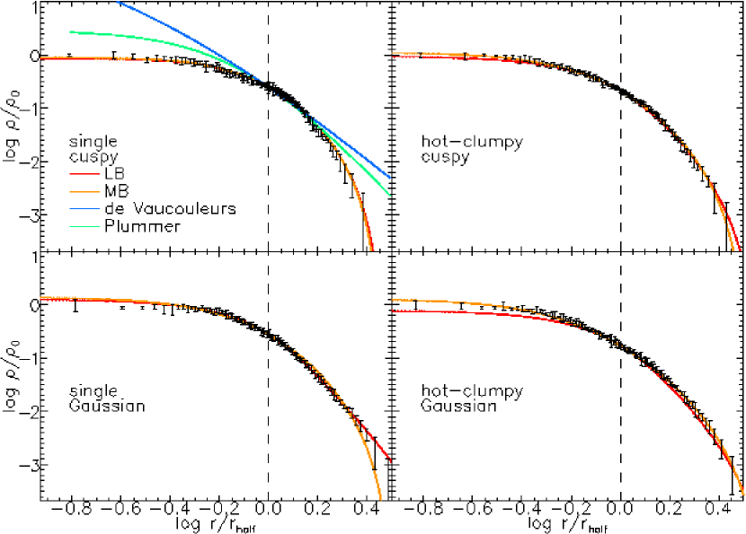
Figure 1.— Logarithmic density profiles for individual $N=10^{5}$ GADGET simulations with $Q_{0}=1.0$. The radial coordinate is scaled by the half-mass radius (indicated by the vertical dashed line) in all profiles. In each panel, the initial conditions are specified and the errorbars indicate the data values from the simulations. The curves show the behaviors of the various models, specified in the legend. As they provide poor descriptions of the simulations, the Plummer and de Vaucouleurs models are only included in the single cuspy panel for reference. Lynden-Bell (LB) model fits produce density $\chi_{r}^{2}$ values smaller or comparable to those with Maxwell-Boltzmann (MB) models (except for the hot-clumpy Gaussian simulation): single cuspy – $\chi_{\rm LB}^{2}=0.635$, $\chi_{\rm MB}^{2}=0.635$; single Gaussian – $\chi_{\rm LB}^{2}=0.811$, $\chi_{\rm MB}^{2}=2.162$; hot-clumpy cuspy – $\chi_{\rm LB}^{2}=1.207$, $\chi_{\rm MB}^{2}=0.554$; hot-clumpy Gaussian – $\chi_{\rm LB}^{2}=5.093$, $\chi_{\rm MB}^{2}=0.581$.

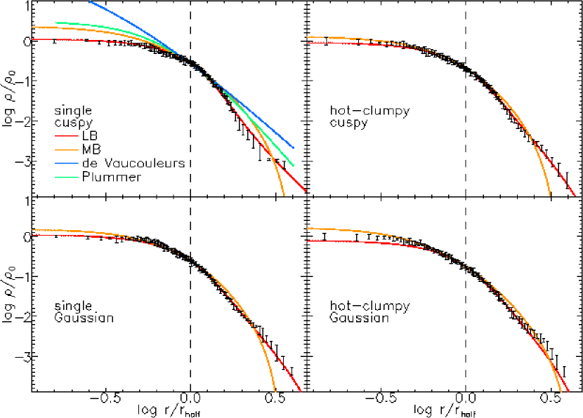
Figure 2.— Logarithmic density profiles for individual $N=10^{5}$ GADGET simulations with $Q_{0}=0.7$. The panels and linestyles are the same as in Figure 1. In these simulations, the density profiles share a slight upward concavity in their outer profile. In general, the LB model fits are able to match this data behavior better than the MB models: single cuspy – $\chi_{\rm LB}^{2}=1.503$, $\chi_{\rm MB}^{2}=9.218$; single Gaussian – $\chi_{\rm LB}^{2}=0.903$, $\chi_{\rm MB}^{2}=4.847$; hot-clumpy cuspy – $\chi_{\rm LB}^{2}=0.777$, $\chi_{\rm MB}^{2}=4.332$; hot-clumpy Gaussian – $\chi_{\rm LB}^{2}=3.204$, $\chi_{\rm MB}^{2}=3.360$.

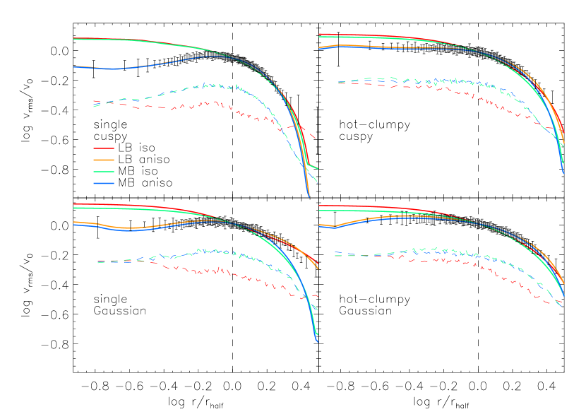
Figure 3.— Logarithmic $v_{\rm rms}$ profiles for individual $N=10^{5}$ GADGET simulations with $Q_{0}=1.0$. Again, the radial coordinate is scaled by the half-mass radius (vertical dashed line). As before, the initial conditions are specified in each panel, and the errorbars indicate the data values from the simulations. The thin lines that appear below the errorbars show the behaviors of $v_{{\rm rms},r}$ (the lowest line) and the nearly identical $v_{{\rm rms},\theta}$ and $v_{{\rm rms},\phi}$. From these components, one can see the mild tangential velocity anisotropy that exists in these simulated equilibria. Two sets of model curves are shown superimposed with the data. As indicated in the legend in the upper-left panel, there are isotropic and anisotropic model results. Isotropic model profiles reach nearly constant values near the centers of systems, while anisotropic model profiles provide better representations of the data for smaller $r$. In general, anisotropic LB models produce the smallest velocity $\chi_{r}^{2}$ values: single cuspy – $\chi_{\rm LB,iso}^{2}=1.108$, $\chi_{\rm LB,aniso}^{2}=0.036$, $\chi_{\rm MB,iso}^{2}=1.072$, $\chi_{\rm MB,aniso}^{2}=0.050$; single Gaussian – $\chi_{\rm LB,iso}^{2}=1.087$, $\chi_{\rm LB,aniso}^{2}=0.078$, $\chi_{\rm MB,iso}^{2}=1.778$, $\chi_{\rm MB,aniso}^{2}=0.832$; hot-clumpy cuspy – $\chi_{\rm LB,iso}^{2}=0.466$, $\chi_{\rm LB,aniso}^{2}=0.016$, $\chi_{\rm MB,iso}^{2}=0.500$, $\chi_{\rm MB,aniso}^{2}=0.087$; hot-clumpy Gaussian – $\chi_{\rm LB,iso}^{2}=0.447$, $\chi_{\rm LB,aniso}^{2}=0.038$, $\chi_{\rm MB,iso}^{2}=0.325$, $\chi_{\rm MB,aniso}^{2}=0.033$. Coupled with the generally better density fits provided by the LB models, these velocity fits suggest that the LB models are the superior description of the phase-space distributions of these simulations.

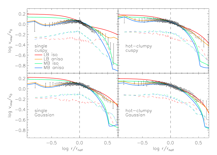
Figure 4.— Logarithmic $v_{\rm rms}$ profiles for individual $N=10^{5}$ GADGET simulations with $Q_{0}=0.7$. The panels here are analogous to those in Figure 3. The ineffectiveness of isotropic models remains evident, and the superiority of anisotropic LB models is even clearer than in the $Q_{0}=1.0$ cases: single cuspy – $\chi_{\rm LB,iso}^{2}=2.231$, $\chi_{\rm LB,aniso}^{2}=0.214$, $\chi_{\rm MB,iso}^{2}=1.024$, $\chi_{\rm MB,aniso}^{2}=0.644$; single Gaussian – $\chi_{\rm LB,iso}^{2}=0.953$, $\chi_{\rm LB,aniso}^{2}=0.072$, $\chi_{\rm MB,iso}^{2}=1.393$, $\chi_{\rm MB,aniso}^{2}=1.724$; hot-clumpy cuspy – $\chi_{\rm LB,iso}^{2}=0.696$, $\chi_{\rm LB,aniso}^{2}=0.043$, $\chi_{\rm MB,iso}^{2}=1.866$, $\chi_{\rm MB,aniso}^{2}=3.254$; hot-clumpy Gaussian – $\chi_{\rm LB,iso}^{2}=0.324$, $\chi_{\rm LB,aniso}^{2}=0.167$, $\chi_{\rm MB,iso}^{2}=0.546$, $\chi_{\rm MB,aniso}^{2}=1.130$.

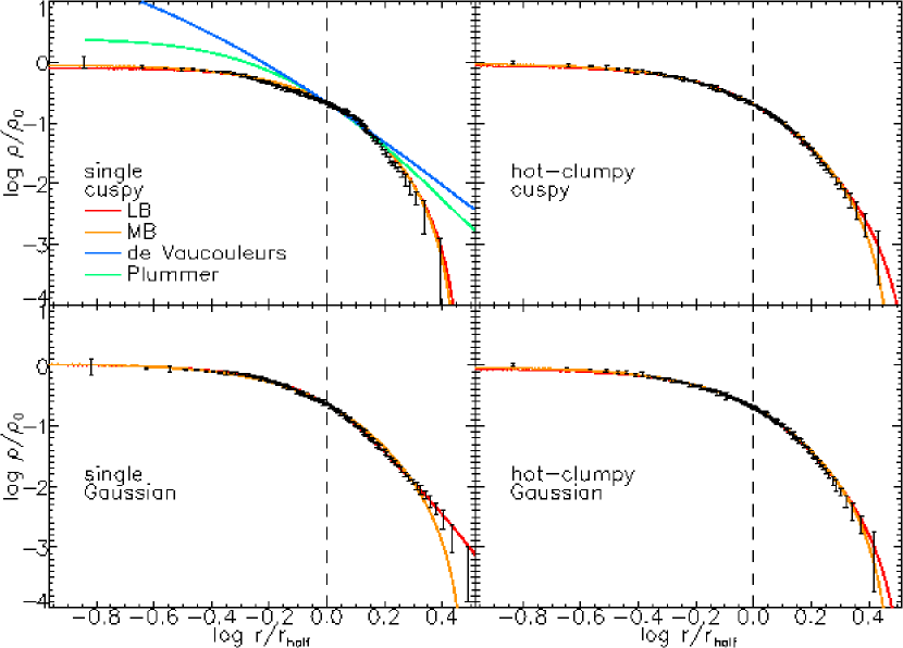
Figure 5.— Logarithmic density profiles for averaged $N=10^{5}$ GADGET simulations with $Q_{0}=1.0$. The panels are analogous to those in Figure 1. The errorbars marking the data points are smaller and the data points show less point-to-point variation than in Figure 1. As before, the LB models tend to provide better descriptions of the data: single cuspy – $\chi_{\rm LB}^{2}=4.569$, $\chi_{\rm MB}^{2}=4.438$; single Gaussian – $\chi_{\rm LB}^{2}=0.635$, $\chi_{\rm MB}^{2}=3.182$; hot-clumpy cuspy – $\chi_{\rm LB}^{2}=0.769$, $\chi_{\rm MB}^{2}=0.652$; hot-clumpy Gaussian – $\chi_{\rm LB}^{2}=1.389$, $\chi_{\rm MB}^{2}=0.754$.

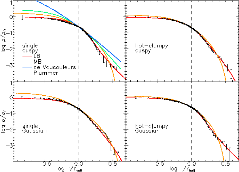
Figure 6.— Logarithmic density profiles for averaged $N=10^{5}$ GADGET simulations with $Q_{0}=0.7$. The panels are analogous to those in Figure 2, and the data profiles present smoother versions of the outer-profile concavity features seen there. Again, the LB models tend to describe the data behavior more completely than the MB models: single cuspy – $\chi_{\rm LB}^{2}=7.658$, $\chi_{\rm MB}^{2}=44.058$; single Gaussian – $\chi_{\rm LB}^{2}=3.346$, $\chi_{\rm MB}^{2}=28.463$; hot-clumpy cuspy – $\chi_{\rm LB}^{2}=0.788$, $\chi_{\rm MB}^{2}=7.670$; hot-clumpy Gaussian – $\chi_{\rm LB}^{2}=2.215$, $\chi_{\rm MB}^{2}=9.064$.

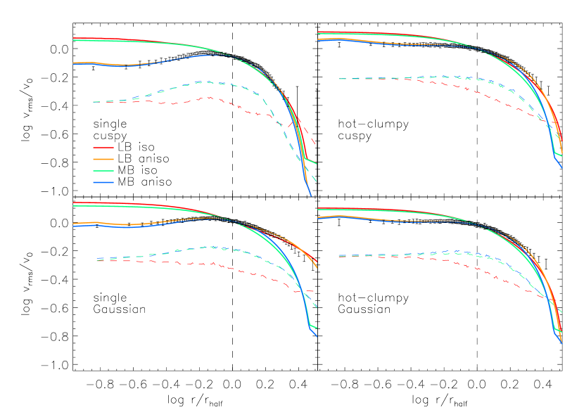
Figure 7.— Logarithmic $v_{\rm rms}$ profiles for averaged $N=10^{5}$ GADGET simulations with $Q_{0}=1.0$. The panels are analogous to those in Figure 3. These smoother versions again indicate that models incorporating the velocity anisotropy present in the simulations are better suited to describing the data. Of the models considered here, the anisotropic LB models provide the best representation of the data: single cuspy – $\chi_{\rm LB,iso}^{2}=5.866$, $\chi_{\rm LB,aniso}^{2}=0.370$, $\chi_{\rm MB,iso}^{2}=5.629$, $\chi_{\rm MB,aniso}^{2}=0.424$; single Gaussian – $\chi_{\rm LB,iso}^{2}=6.326$, $\chi_{\rm LB,aniso}^{2}=0.121$, $\chi_{\rm MB,iso}^{2}=9.294$, $\chi_{\rm MB,aniso}^{2}=3.013$; hot-clumpy cuspy – $\chi_{\rm LB,iso}^{2}=2.521$, $\chi_{\rm LB,aniso}^{2}=0.080$, $\chi_{\rm MB,iso}^{2}=3.319$, $\chi_{\rm MB,aniso}^{2}=0.567$; hot-clumpy Gaussian – $\chi_{\rm LB,iso}^{2}=3.137$, $\chi_{\rm LB,aniso}^{2}=0.087$, $\chi_{\rm MB,iso}^{2}=3.531$, $\chi_{\rm MB,aniso}^{2}=0.357$.

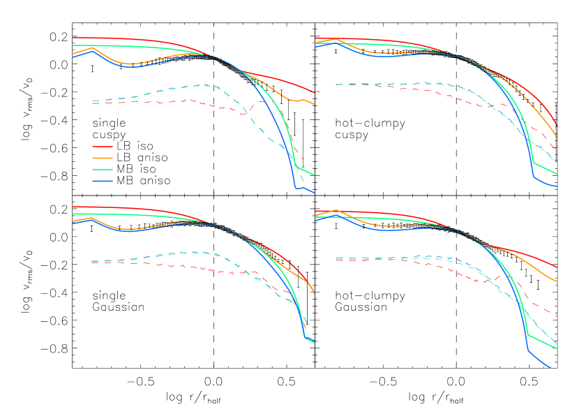
Figure 8.— Logarithmic $v_{\rm rms}$ profiles for averaged $N=10^{5}$ GADGET simulations with $Q_{0}=0.7$. These panels are analogous to those in Figure 4. The smaller errorbars in these simulations result in some poorer fits between the anisotropic LB model and the data (e.g.,in the clumpy Gaussian simulation, lower-right panel): single cuspy – $\chi_{\rm LB,iso}^{2}=8.069$, $\chi_{\rm LB,aniso}^{2}=0.730$, $\chi_{\rm MB,iso}^{2}=3.699$, $\chi_{\rm MB,aniso}^{2}=1.029$; single Gaussian – $\chi_{\rm LB,iso}^{2}=4.240$, $\chi_{\rm LB,aniso}^{2}=0.341$, $\chi_{\rm MB,iso}^{2}=1.945$, $\chi_{\rm MB,aniso}^{2}=2.021$; hot-clumpy cuspy – $\chi_{\rm LB,iso}^{2}=2.779$, $\chi_{\rm LB,aniso}^{2}=0.214$, $\chi_{\rm MB,iso}^{2}=6.954$, $\chi_{\rm MB,aniso}^{2}=10.852$; hot-clumpy Gaussian – $\chi_{\rm LB,iso}^{2}=2.913$, $\chi_{\rm LB,aniso}^{2}=0.331$, $\chi_{\rm MB,iso}^{2}=2.872$, $\chi_{\rm MB,aniso}^{2}=3.970$.

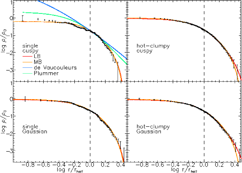
Figure 9.— Logarithmic density profiles for individual $N=10^{6}$ GADGET simulations with $Q_{0}=1.0$. These panels are analogous to those in Figure 1. The point-to-point variations seen in the single simulations can be relatively large, leading us to question the appropriateness of our estimated data point uncertainties. However, the clumpy simulation results are quite smooth, and at least on a relative basis, the LB models describe the data better than the MB models: single cuspy – $\chi_{\rm LB}^{2}=15.891$, $\chi_{\rm MB}^{2}=16.596$; single Gaussian – $\chi_{\rm LB}^{2}=6.956$, $\chi_{\rm MB}^{2}=7.218$; hot-clumpy cuspy – $\chi_{\rm LB}^{2}=0.844$, $\chi_{\rm MB}^{2}=0.859$; hot-clumpy Gaussian – $\chi_{\rm LB}^{2}=0.561$, $\chi_{\rm MB}^{2}=1.364$.

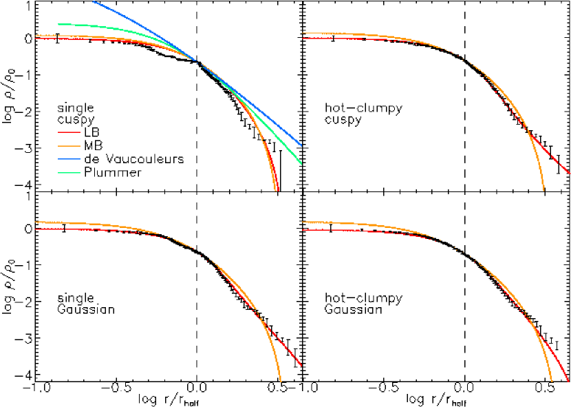
Figure 10.— Logarithmic density profiles for individual $N=10^{6}$ GADGET simulations with $Q_{0}=0.7$. These panels are analogous to those in Figure 2. Again, the data points for clumpy simulations show a smoothness not present in the single simulations. Except for the single cuspy simulation, the LB models clearly provide a superior description of the data: single cuspy – $\chi_{\rm LB}^{2}=81.184$, $\chi_{\rm MB}^{2}=105.158$; single Gaussian – $\chi_{\rm LB}^{2}=3.572$, $\chi_{\rm MB}^{2}=32.259$; hot-clumpy cuspy – $\chi_{\rm LB}^{2}=1.999$, $\chi_{\rm MB}^{2}=28.178$; hot-clumpy Gaussian – $\chi_{\rm LB}^{2}=2.730$, $\chi_{\rm MB}^{2}=22.357$.

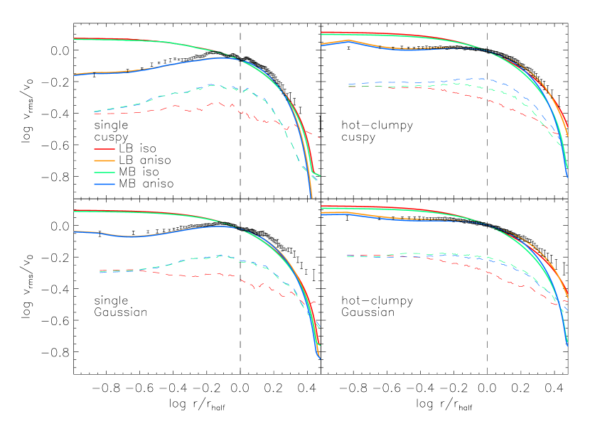
Figure 11.— Logarithmic $v_{\rm rms}$ profiles for individual $N=10^{6}$ GADGET simulations with $Q_{0}=1.0$. These panels are analogous to those in Figure 3. The models with velocity isotropy continue to be poor descriptors of the data, while the anisotropic LB models provide the best fits to the simulation results: single cuspy – $\chi_{\rm LB,iso}^{2}=16.044$, $\chi_{\rm LB,aniso}^{2}=2.962$, $\chi_{\rm MB,iso}^{2}=15.723$, $\chi_{\rm MB,aniso}^{2}=3.188$; single Gaussian – $\chi_{\rm LB,iso}^{2}=12.313$, $\chi_{\rm LB,aniso}^{2}=3.004$, $\chi_{\rm MB,iso}^{2}=12.135$, $\chi_{\rm MB,aniso}^{2}=3.733$; hot-clumpy cuspy – $\chi_{\rm LB,iso}^{2}=7.312$, $\chi_{\rm LB,aniso}^{2}=0.205$, $\chi_{\rm MB,iso}^{2}=6.728$, $\chi_{\rm MB,aniso}^{2}=0.727$; hot-clumpy Gaussian – $\chi_{\rm LB,iso}^{2}=3.574$, $\chi_{\rm LB,aniso}^{2}=0.153$, $\chi_{\rm MB,iso}^{2}=4.383$, $\chi_{\rm MB,aniso}^{2}=1.226$.

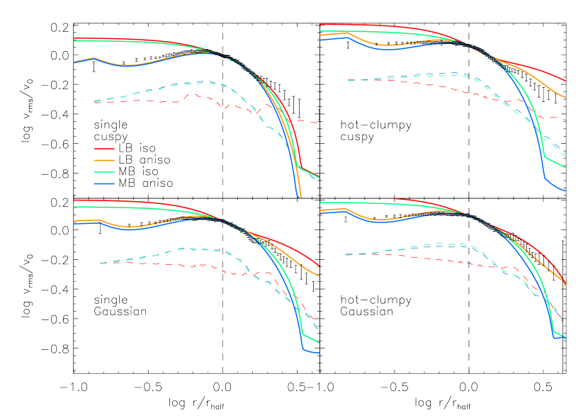
Figure 12.— Logarithmic $v_{\rm rms}$ profiles for individual $N=10^{6}$ GADGET simulations with $Q_{0}=0.7$. These panels are analogous to those in Figure 4. Again, the anisotropic LB models provide the best descriptions of the data (even though it appears to under-predict the single cuspy simulation results for larger $r$): single cuspy – $\chi_{\rm LB,iso}^{2}=12.735$, $\chi_{\rm LB,aniso}^{2}=1.824$, $\chi_{\rm MB,iso}^{2}=9.868$, $\chi_{\rm MB,aniso}^{2}=2.985$; single Gaussian – $\chi_{\rm LB,iso}^{2}=17.030$, $\chi_{\rm LB,aniso}^{2}=0.740$, $\chi_{\rm MB,iso}^{2}=7.721$, $\chi_{\rm MB,aniso}^{2}=2.673$; hot-clumpy cuspy – $\chi_{\rm LB,iso}^{2}=13.464$, $\chi_{\rm LB,aniso}^{2}=0.806$, $\chi_{\rm MB,iso}^{2}=5.429$, $\chi_{\rm MB,aniso}^{2}=2.756$; hot-clumpy Gaussian – $\chi_{\rm LB,iso}^{2}=15.484$, $\chi_{\rm LB,aniso}^{2}=0.756$, $\chi_{\rm MB,iso}^{2}=7.722$, $\chi_{\rm MB,aniso}^{2}=2.308$.

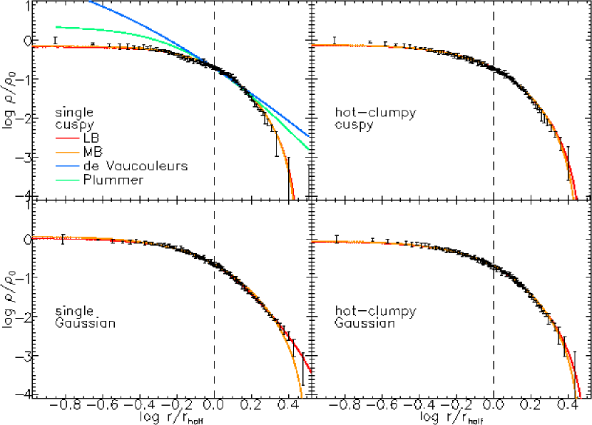
Figure 13.— Logarithmic density profiles for individual $N=2^{17}$ GPU-NBODY-6 simulations with $Q_{0}=1.0$. These panels are analogous to those in Figure 1. Evolving systems with this non-softened code produces equilibria with density profiles that are nearly indistinguishable from those discussed earlier. As with the GADGET results, LB models provide better representations of the data: single cuspy – $\chi_{\rm LB}^{2}=1.952$, $\chi_{\rm MB}^{2}=2.064$; single Gaussian – $\chi_{\rm LB}^{2}=0.390$, $\chi_{\rm MB}^{2}=1.537$; hot-clumpy cuspy – $\chi_{\rm LB}^{2}=1.096$, $\chi_{\rm MB}^{2}=0.964$; hot-clumpy Gaussian – $\chi_{\rm LB}^{2}=0.595$, $\chi_{\rm MB}^{2}=0.584$.

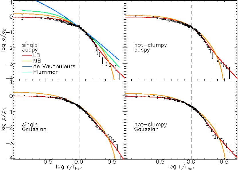
Figure 14.— Logarithmic density profiles for individual $N=2^{17}$ GPU-NBODY-6 simulations with $Q_{0}=0.7$. These panels are analogous to those in Figure 2. The fact that the LB models can reproduce the slight concave features in the outer regions of the profiles again lead to them being preferred to the MB models: single cuspy – $\chi_{\rm LB}^{2}=3.653$, $\chi_{\rm MB}^{2}=17.118$; single Gaussian – $\chi_{\rm LB}^{2}=1.420$, $\chi_{\rm MB}^{2}=13.025$; hot-clumpy cuspy – $\chi_{\rm LB}^{2}=3.191$, $\chi_{\rm MB}^{2}=13.159$; hot-clumpy Gaussian – $\chi_{\rm LB}^{2}=0.735$, $\chi_{\rm MB}^{2}=8.175$.

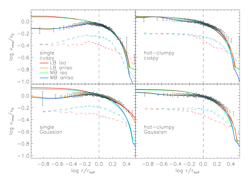
Figure 15.— Logarithmic $v_{\rm rms}$ profiles for individual $N=2^{17}$ GPU-NBODY-6 simulations with $Q_{0}=1.0$. These panels are analogous to those in Figure 3. The trend for anisotropic LB models to provide the best description of the $v_{\rm rms}$ data continues. Note that the clumpy cuspy simulation results in a nearly isotropic velocity distribution, and that the inner part of the profile is decently well-described by the isotropic LB prediction: single cuspy – $\chi_{\rm LB,iso}^{2}=1.741$, $\chi_{\rm LB,aniso}^{2}=0.048$, $\chi_{\rm MB,iso}^{2}=1.639$, $\chi_{\rm MB,aniso}^{2}=0.058$; single Gaussian – $\chi_{\rm LB,iso}^{2}=0.904$, $\chi_{\rm LB,aniso}^{2}=0.032$, $\chi_{\rm MB,iso}^{2}=1.734$, $\chi_{\rm MB,aniso}^{2}=0.953$; hot-clumpy cuspy – $\chi_{\rm LB,iso}^{2}=0.508$, $\chi_{\rm LB,aniso}^{2}=0.194$, $\chi_{\rm MB,iso}^{2}=0.711$, $\chi_{\rm MB,aniso}^{2}=0.310$; hot-clumpy Gaussian – $\chi_{\rm LB,iso}^{2}=1.278$, $\chi_{\rm LB,aniso}^{2}=0.192$, $\chi_{\rm MB,iso}^{2}=1.787$, $\chi_{\rm MB,aniso}^{2}=0.560$.

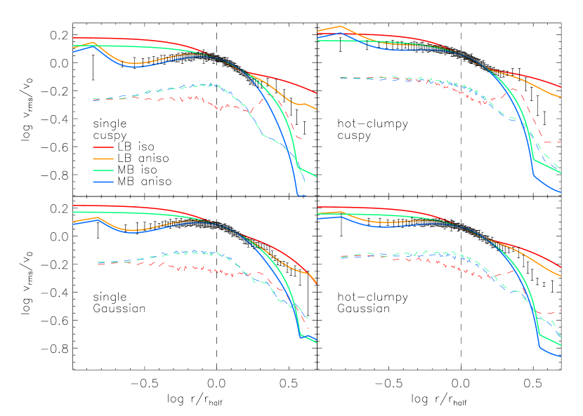
Figure 16.— Logarithmic $v_{\rm rms}$ profiles for individual $N=2^{17}$ GPU-NBODY-6 simulations with $Q_{0}=0.7$. These panels are analogous to those in Figure 4. The anisotropic LB models continue to represent the data behavior better than the other models considered: single cuspy – $\chi_{\rm LB,iso}^{2}=1.899$, $\chi_{\rm LB,aniso}^{2}=0.128$, $\chi_{\rm MB,iso}^{2}=0.863$, $\chi_{\rm MB,aniso}^{2}=0.725$; single Gaussian – $\chi_{\rm LB,iso}^{2}=1.956$, $\chi_{\rm LB,aniso}^{2}=0.114$, $\chi_{\rm MB,iso}^{2}=1.365$, $\chi_{\rm MB,aniso}^{2}=1.772$; hot-clumpy cuspy – $\chi_{\rm LB,iso}^{2}=0.516$, $\chi_{\rm LB,aniso}^{2}=0.147$, $\chi_{\rm MB,iso}^{2}=0.665$, $\chi_{\rm MB,aniso}^{2}=1.177$; hot-clumpy Gaussian – $\chi_{\rm LB,iso}^{2}=1.560$, $\chi_{\rm LB,aniso}^{2}=0.384$, $\chi_{\rm MB,iso}^{2}=0.877$, $\chi_{\rm MB,aniso}^{2}=1.306$.

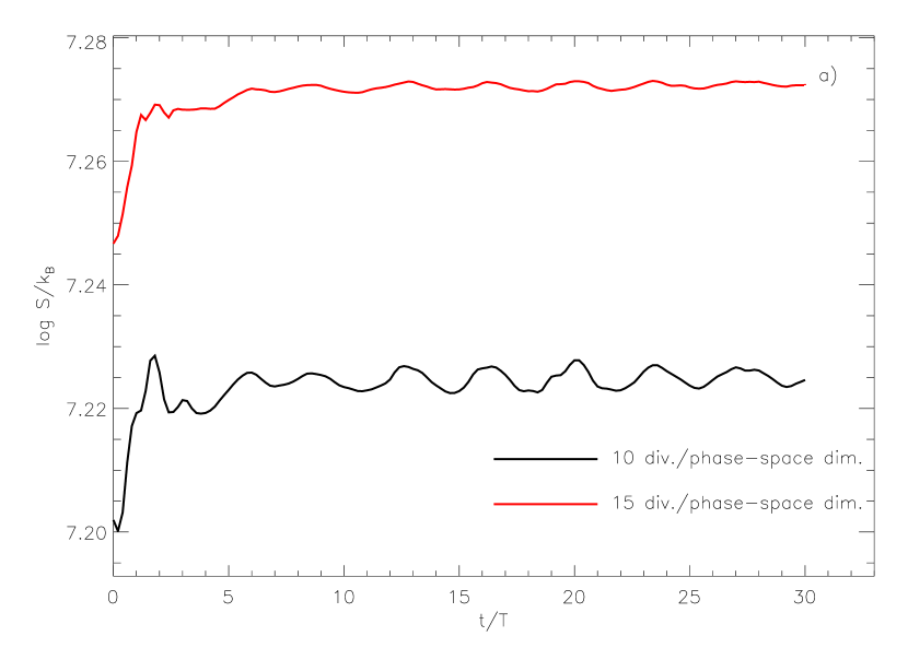
Figure 17.— (a) Lynden-Bell entropy versus time in the individual single, cuspy $N=10^{6}$ GADGET simulation with $Q_{0}=0.7$. The entropy is calculated from the phase-space macro-cell occupation values (Equation 4), with a value of $\nu_{\rm LB}=10^{4}$. Two different macro-cell volumes (indicated in the legend) have been used to create comparison curves. Adopting a smaller macro-cell volume increases the zero point of the curve and reduces the small-scale variations in $S_{\rm LB}$ but leaves the overall behavior unchanged. (b) The virial ratio $Q$ as a function of time for the same simulation. The initial increase in $S_{\rm LB}$ appears to coincide with the initial growth in $Q$.

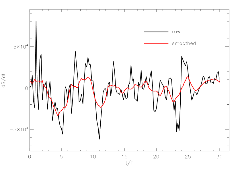
Figure 18.— The macroscopic entropy production rate versus time in the individual single, cuspy $N=10^{6}$ GADGET simulation with $Q_{0}=0.7$. The production rate is calculated by determining gradients in the kinetic temperature and mean velocity field (Equation 8). The rather coarse grid used to determine the gradients may play an important role in the essentially null result shown. If the macroscopic entropy production could be properly calculated, one would expect a rather large positive spike in the interval $0\leq t/T\lesssim 5$.

References

- Barnes, Lanzel, & Williams (2009) Barnes, E. I., Lanzel, P. A., Williams, L. L. R. 2009, ApJ, 704, 372
- Barnes & Williams (2011) Barnes, E. I., Williams, L. L. R. 2011, ApJ, 728, 136
- Barnes & Williams (2012) Barnes, E. I., Williams, L. L. R. 2012, ApJ, 748, 144
- Binney & Tremaine (1987) Binney, J., Tremaine, S. 1987, Galactic Dynamics, (Princeton, NJ:Princeton)
- de Groot & Mazur (1984) de Groot, S. R., Mazur, P. 1984, Non-Equilibrium Thermodynamics, (Mineola, NY:Dover)
- de Vaucouleurs (1948) de Vaucouleurs, G. 1948, Ann. d’Astrophys., 11, 247
- Lynden-Bell (1967) Lynden-Bell, D. 1967, MNRAS, 136, 101
- Merritt (1985) Merritt, D. 1985, AJ, 90, 1027
- Merritt & Aguilar (1985) Merritt, D., Aguilar, L. A. 1985, MNRAS, 217, 787
- Moore et al. (1999) Moore, B., Quinn, T., Governato, F., Stadel, J., Lake, G., 1999, MNRAS, 310, 1147
- Navarro, Frenk, & White (1996) Navarro, J. F., Frenk, C. S., White, S. D. M. 1996, ApJ, 462, 563
- Navarro, Frenk, & White (1997) Navarro, J. F., Frenk, C. S., White, S. D. M. 1997, ApJ, 490, 493
- Navarro et al. (2004) Navarro, J. F., Hayashi, E., Power, C., Jenkins, A. R., Frenk, C. S., White, S. D. M., Springel, V., Stadel, J., Quinn, T. R. 2004, MNRAS, 349, 1039
- Nitadori & Aarseth (2012) Nitadori, K., Aarseth, S. 2012, MNRAS, 424, 545
- Plummer (1911) Plummer, H. C. 1911, MNRAS, 72, 460
- Power et al. (2003) Power, C., Navarro, J. F., Jenkins, A., Frenk, C. S., White, S. D. M., Springel, V., Stadel, J., Quinn, T. 2003, MNRAS, 338, 14
- Press et al. (1994) Press, W.H., Teukolsky, S.A., Vetterling, W.T., Flannery, B.P. 1994, Numerical Recipes, Cambridge Univ. Press: New York, NY
- Springel (2005) Springel, V. 2005, MNRAS, 364, 1105
- Springel et al. (2005) Springel, V., White, S. D. M., Jenkins, A., Frenk, C. S., Yoshida, N., Gao, L., Navarro, J., Thacker, R., Croton, D., Helly, J., Peacock, J. A., Cole, S., Thomas, P., Couchman, H., Evrard, A., Colberg, J., Pearce, F. 2005, Nature, 435, 629
- Sylos Labini (2012) Sylos Labini, F. 2012, MNRAS, 423, 1610
- Taylor & Navarro (2001) Taylor, J. E., Navarro, J. F. 2001, ApJ, 563, 483
- Trenti & Bertin (2005) Trenti, M., Bertin, G. 2005, A&A, 429, 161
- van Albada (1982) van Albada, T. S. 1982, MNRAS, 201, 939