Global minima for semilinear optimal control problems

Abstract: We consider an optimal control problem subject to a semilinear elliptic PDE together with its variational discretization. We provide a condition which allows to decide whether a solution of the necessary first order conditions is a global minimum. This condition can be explicitly evaluated at the discrete level. Furthermore, we prove that if the above condition holds uniformly with respect to the discretization parameter the sequence of discrete solutions converges to a global solution of the corresponding limit problem. Numerical examples with unique global solutions are presented.
Mathematics Subject Classification (2000): 49J20, 35K20, 49M05, 49M25, 49M29, 65M12, 65M60
Keywords: Optimal control, semilinear PDE, uniqueness of global solutions, Gagliardo–Nirenberg inequality

1 Introduction

Let us consider the following optimal control problem

$$(\mathbb{P})\quad\min_{u\in U_{ad}}J(u)=\frac{1}{2}\|y-y_{0}\|_{L^{2}(\Omega)}^{2}+\dfrac{\alpha}{2}\|u\|_{L^{2}(\Omega)}^{2}$$

subject to the semilinear elliptic PDE

$$-\Delta y+\phi(y) =u\quad\mbox{ in }\Omega\subset\mathbb{R}^{2},$$ (1.1)

$$y =0\quad\mbox{ on }\partial\Omega,$$

and the pointwise state constraints

$$y_{a}(x)\leq y(x)\leq y_{b}(x),\quad x\in K\subset\Omega.$$ (1.2)

We will formulate the precise assumptions on the data of the problem in Section 2. Since the state equation is in general nonlinear, the control problem is nonconvex and there may be several solutions of the necessary first order conditions. These can be examined further with the help of second order conditions but those will only give local information and usually do not allow a decision on whether the given point is a global minimum of $\displaystyle(\mathbb{P})$. It is exactly this question which is the starting point of our work. Assuming that we have an admissible control $\displaystyle\bar{u}$ which satisfies the necessary first order conditions we will formulate a condition on the adjoint variable that guarantees that $\displaystyle\bar{u}$ is a solution of the control problem $\displaystyle(\mathbb{P})$. This condition requires a certain $\displaystyle L^{q}$–norm to be bounded by a constant that only depends on the data and that is known explicitly. While this approach is only of limited use at the continuous level, the situation is different when we apply our methods to a suitable discretisation $\displaystyle(\mathbb{P}_{h})$ of $\displaystyle(\mathbb{P})$. It turns out that we can obtain an analogous result for a discrete stationary point $\displaystyle\bar{u}_{h}$ and the corresponding discrete adjoint state. But since now the discrete adjoint is available to us as a result of a numerical computation, we can check whether our condition is satisfied. If the answer is yes, $\displaystyle\bar{u}_{h}$ is a global minimum of $\displaystyle(\mathbb{P}_{h})$. Moreover we are able to make the connection back to the original control problem in that we show that a sequence of solutions of $\displaystyle(\mathbb{P}_{h})$, that satisfy our condition uniformly in $\displaystyle h$ converge to a global solution of $\displaystyle(\mathbb{P})$.

To the best of the author’s knowledge this is the first contribution to the study of uniqueness of solutions to semilinear elliptic optimal control problems. However, concerning the analysis, numerical treatment and implementation of semilinear optimal control problems many contributions can be found in the literature. Here we exemplarily mention the work [1] of Arada et al., [2] of Casas, and the work [11] of Neitzel et al. Further references can be found in [9, Chapter 3], [8], and in [3], where the role of second order conditions in PDE constrained optimization is discussed.

2 The optimal control problem $\displaystyle(\mathbb{P})$

Let $\displaystyle\Omega\subset\mathbb{R}^{2}$ be a bounded, convex and polygonal domain. We assume that $\displaystyle\phi:\mathbb{R}\to\mathbb{R}$ is of class $\displaystyle C^{2}$ and monotonically increasing. For our analysis we require the following structural assumption on $\displaystyle\phi$:
Assumption 1: There exist $\displaystyle r>1$ and $\displaystyle M\geq 0$ such that

$$|\phi^{\prime\prime}(s)|\leq M\phi^{\prime}(s)^{\frac{1}{r}}\quad\mbox{ for all }s\in\mathbb{R}.$$ (2.1)

Let us remark for later purposes that (2.1) implies

$$\displaystyle\phi^{\prime}(s) \displaystyle\leq \displaystyle c_{1}\bigl{(}1+|s|^{r_{1}}\bigr{)},\;s\in\mathbb{R},\quad r_{1}=\frac{r}{r-1}$$ (2.2)

$$\displaystyle|\phi(s)| \displaystyle\leq \displaystyle c_{0}\bigl{(}1+|s|^{r_{0}}\bigr{)},\;s\in\mathbb{R},\quad r_{0}=\frac{2r-1}{r-1}.$$ (2.3)

Note that for a power nonlinearity of the form $\displaystyle\phi(s)=|s|^{q-2}s$ ($\displaystyle q>3$)

$$|\phi^{\prime\prime}(s)|=(q-1)(q-2)|s|^{q-3}=(q-2)(q-1)^{\frac{1}{q-2}}[\phi^{\prime}(s)]^{\frac{q-3}{q-2}},$$

so that (2.1) is satisfied if we chose $\displaystyle r=\tfrac{q-2}{q-3}$. Solving this relation for $\displaystyle q$ yields $\displaystyle q=\tfrac{3r-2}{r-1}$, which is an expression that we will encounter in our analysis below.
Using the theory of monotone operators one can show that for every $\displaystyle u\in L^{2}(\Omega)$ the boundary value problem (1.1) has a unique solution $\displaystyle y\in H^{1}_{0}(\Omega)\cap H^{2}(\Omega)$ which we denote by $\displaystyle y=\mathcal{G}(u)$. Moreover, there exists a constant $\displaystyle c>0$ such that

$$\|y\|_{H^{2}(\Omega)}\leq c\bigl{(}1+\|u\|_{L^{2}(\Omega)}\bigr{)}.$$

Next, suppose that $\displaystyle K$ is a (possibly empty) compact subset of $\displaystyle\Omega$ and define

$$Y_{ad}:=\{z\in C(K):y_{a}(x)\leq z(x)\leq y_{b}(x)\mbox{ for all }x\in K\}.$$

Here, $\displaystyle y_{a},y_{b}\in C_{0}(\Omega)$ are given functions that satisfy $\displaystyle y_{a}(x)<y_{b}(x),x\in K$.
We consider the semilinear optimal control problem

$$(\mathbb{P})\quad\begin{array}[]{l}\min_{u\in U_{ad}}J(u):=\frac{1}{2}\|y-y_{0}\|_{L^{2}(\Omega)}^{2}+\dfrac{\alpha}{2}\|u\|_{L^{2}(\Omega)}^{2}\\ \mbox{ subject to }y=\mathcal{G}(u)\mbox{ and }y_{|K}\in Y_{ad},\end{array}$$

where

$$U_{ad}:=\{u\in L^{2}(\Omega):u_{a}\leq u(x)\leq u_{b}\mbox{ a.e. in }\Omega\}$$

and $\displaystyle-\infty\leq u_{a}\leq u_{b}\leq\infty$ are given. By classical arguments Problem $\displaystyle(\mathbb{P})$ has a solution $\displaystyle\bar{u}\in U_{ad}$.

Remark 1 

We note that the choice $\displaystyle K=\bar{\Omega}$ also is possible, if the bounds satisfy the compatibility condition $\displaystyle y_{a}<0<y_{b}$ on $\displaystyle\partial\Omega$, which only requires minor modifications in the analysis.

3 The variational discretization of $\displaystyle(\mathbb{P})$

In this section we approximate Problem $\displaystyle(\mathbb{P})$ using the variational discretization approach introduced in [7]. To this end, let $\displaystyle\mathcal{T}_{h}$ be an admissible triangulation of $\displaystyle\Omega$ so that

$$\bar{\Omega}=\bigcup_{T\in\mathcal{T}_{h}}\bar{T}.$$

We define the space of linear finite elements,

$$X_{h0}:=\{v_{h}\in C(\bar{\Omega}):v_{h}\mbox{ is a linear polynomial on each }T\in\mathcal{T}_{h}\mbox{ and }{v_{h}}_{|\partial\Omega}=0\}$$

and approximate (1.1) as follows: for a given $\displaystyle u\in L^{2}(\Omega)$, find $\displaystyle y_{h}\in X_{h0}$ such that

$$\int_{\Omega}\nabla y_{h}\cdot\nabla v_{h}+\phi(y_{h})v_{h}\,dx=\int_{\Omega}uv_{h}\,dx\quad\forall\,v_{h}\in X_{h0}.$$ (3.1)

Using a fixed point argument one can show that (3.1) has a unique solution $\displaystyle y_{h}\in X_{h0}$ which we denote by $\displaystyle\mathcal{G}_{h}(u)$. Finally, let us define

$$\mathcal{N}_{h}:=\{x_{j}\,|\,x_{j}\mbox{ is a vertex of }T\in\mathcal{T}_{h},\mbox{ where }T\cap K\neq\emptyset\}.$$

The variational discretization of Problem $\displaystyle(\mathbb{P})$ now reads:

$$(\mathbb{P}_{h})\quad\begin{array}[]{l}\min_{u\in U_{ad}}J_{h}(u):=\frac{1}{2}\|y_{h}-y_{0}\|_{L^{2}(\Omega)}^{2}+\dfrac{\alpha}{2}\|u\|_{L^{2}(\Omega)}^{2}\\ \mbox{ subject to }y_{h}=\mathcal{G}_{h}(u),(y_{h}(x_{j}))_{x_{j}\in\mathcal{N}_{h}}\in Y^{h}_{ad},\end{array}$$

where

$$Y^{h}_{ad}:=\{(z_{j})_{x_{j}\in\mathcal{N}_{h}}\,|\,y_{a}(x_{j})\leq z_{j}\leq y_{b}(x_{j}),x_{j}\in\mathcal{N}_{h}\}.$$

We note that Problem $\displaystyle(\mathbb{P}_{h})$ is still an infinite dimensional optimization problem since the controls are sought in $\displaystyle U_{ad}$. If a feasible point for $\displaystyle(\mathbb{P}_{h})$ exists, standard techniques yield the existence of a solution $\displaystyle\bar{u}_{h}\in U_{ad}$ for Problem $\displaystyle(\mathbb{P}_{h})$. The typical approach in order to find an optimum of $\displaystyle(\mathbb{P}_{h})$ consists in trying to determine solutions of the necessary first order conditions. A formal analysis shows that these conditions read in our case: there exist multipliers $\displaystyle\bar{p}_{h}\in X_{h0}$ and $\displaystyle\bar{\mu}_{j}\in\mathbb{R},x_{j}\in\mathcal{N}_{h}$ such that

$$\displaystyle\int_{\Omega}\nabla\bar{y}_{h}\cdot\nabla v_{h}+\phi(\bar{y}_{h})v_{h}\,dx \displaystyle= \displaystyle\int_{\Omega}\bar{u}_{h}v_{h}\,dx\qquad\forall\,v_{h}\in X_{h0},$$ (3.2)

$$\displaystyle\int_{\Omega}\nabla\bar{p}_{h}\cdot\nabla v_{h}+\phi^{\prime}(\bar{y}_{h})\bar{p}_{h}v_{h}\,dx \displaystyle=$$

$$\displaystyle\int_{\Omega}(\bar{y}_{h}-y_{0})v_{h}\,dx+\sum_{x_{j}\in\mathcal{N}_{h}}\bar{\mu}_{j}v_{h}(x_{j})\qquad\forall\,v_{h}\in X_{h0},$$ (3.3)

$$\displaystyle\int_{\Omega}(\bar{p}_{h}+\alpha\bar{u}_{h})(u-\bar{u}_{h})\,dx \displaystyle\geq \displaystyle 0\qquad\forall\,u\in U_{ad},$$ (3.4)

$$\displaystyle\sum_{x_{j}\in\mathcal{N}_{h}}\bar{\mu}_{j}(z_{j}-\bar{y}_{h}(x_{j})) \displaystyle\leq \displaystyle 0\qquad\forall\,(z_{j})_{x_{j}\in\mathcal{N}_{h}}\in Y^{h}_{ad}.$$ (3.5)

Note that condition (3.4) is equivalent to the relation $\displaystyle\bar{u}_{h}=P_{[u_{a},u_{b}]}\bigl{(}-\frac{\bar{p}_{h}}{\alpha}\bigr{)}$, so that the control variable is implicitly discretized and (3.2)–(3.5) amounts to solving a nonlinear finite-dimensional system. In order to state our main result of this section we introduce the following constant:

$$\eta(\alpha,r):=\alpha^{\frac{\rho}{2}}C^{\frac{2-2r}{r}}_{q}M^{-1}\big{(}\frac{r-1}{2r-1}\big{)}^{\frac{1-r}{r}}q^{1/q}r^{1/r}\rho^{\rho/2}(2-\rho)^{\frac{\rho}{2}-1}.$$ (3.6)

Here, $\displaystyle q:=\tfrac{3r-2}{r-1},\,\rho:=\frac{r+q}{rq}$, while $\displaystyle M$ and $\displaystyle r$ appear in (2.1). Furthermore, $\displaystyle C_{q}$ is an upper bound on the optimal constant in the Gagliardo-Nirenberg inequality $\displaystyle\|f\|_{L^{q}}\leq C\|f\|_{L^{2}}^{\frac{2}{q}}\|\nabla f\|_{L^{2}}^{\frac{q-2}{q}}$ ($\displaystyle q\geq 2)$. For our purposes it will be important to specify a constant $\displaystyle C_{q}$ that is as sharp as possible. Lemma 6.3 in the Appendix will give three such bounds, two of which can be found in the literature, while the third is new to the best of our knowledge. Let us now formulate the main result of this section.

Theorem 3.1

Suppose that $\displaystyle\bar{u}_{h}\in U_{ad},\bar{y}_{h}\in X_{h0},\bar{p}_{h}\in X_{h0},(\bar{\mu}_{j})_{x_{j}\in\mathcal{N}_{h}}$ is a solution of (3.2)-(3.5). If

$$\displaystyle\|\bar{p}_{h}\|_{L^{q}(\Omega)}\leq\eta(\alpha,r),$$ (3.7)

then $\displaystyle\bar{u}_{h}$ is a global minimum for Problem $\displaystyle(\mathbb{P}_{h})$. If the inequality (3.7) is strict, then $\displaystyle\bar{u}_{h}$ is the unique global minimum.

Proof:.

Let $\displaystyle u_{h}\in U_{ad}$ be a feasible control, $\displaystyle y_{h}=\mathcal{G}_{h}(u_{h})$ the associated state with $\displaystyle(y_{h}(x_{j}))_{x_{j}\in\mathcal{N}_{h}}\in Y^{h}_{ad}$. We have

$$\displaystyle J_{h}(u_{h})-J_{h}(\bar{u}_{h}) \displaystyle=\frac{1}{2}\|y_{h}-\bar{y}_{h}\|_{L^{2}(\Omega)}^{2}+\dfrac{\alpha}{2}\|u_{h}-\bar{u}_{h}\|_{L^{2}(\Omega)}^{2}+\alpha\int_{\Omega}\bar{u}_{h}(u_{h}-\bar{u}_{h})\,dx$$

$$\displaystyle\quad+\int_{\Omega}(\bar{y}_{h}-y_{0})(y_{h}-\bar{y}_{h})\,dx=:(A)$$

Using $\displaystyle v_{h}:=y_{h}-\bar{y}_{h}$ in (3.3) we get

$$\displaystyle(A) \displaystyle=\frac{1}{2}\|y_{h}-\bar{y}_{h}\|_{L^{2}(\Omega)}^{2}+\dfrac{\alpha}{2}\|u_{h}-\bar{u}_{h}\|_{L^{2}(\Omega)}^{2}+\alpha\int_{\Omega}\bar{u}_{h}(u_{h}-\bar{u}_{h})\,dx$$

$$\displaystyle\quad+\int_{\Omega}\nabla\bar{p}_{h}\cdot\nabla(y_{h}-\bar{y}_{h})+\phi^{\prime}(\bar{y}_{h})\bar{p}_{h}(y_{h}-\bar{y}_{h})\,dx-\sum_{x_{j}\in\mathcal{N}_{h}}\bar{\mu}_{j}(y_{h}(x_{j})-\bar{y}_{h}(x_{j}))$$

$$\displaystyle\geq\frac{1}{2}\|y_{h}-\bar{y}_{h}\|_{L^{2}(\Omega)}^{2}+\dfrac{\alpha}{2}\|u_{h}-\bar{u}_{h}\|_{L^{2}(\Omega)}^{2}+\alpha\int_{\Omega}\bar{u}_{h}(u_{h}-\bar{u}_{h})\,dx$$

$$\displaystyle\quad+\int_{\Omega}\nabla\bar{p}_{h}\cdot\nabla(y_{h}-\bar{y}_{h})+\phi^{\prime}(\bar{y}_{h})\bar{p}_{h}(y_{h}-\bar{y}_{h})\,dx,$$ (3.8)

by (3.5). Using (3.1) for $\displaystyle y_{h}$ and $\displaystyle\bar{y}_{h}$ with test function $\displaystyle\bar{p}_{h}$ we get

$$\displaystyle\int_{\Omega}\nabla\bar{p}_{h}\cdot\nabla(y_{h}-\bar{y}_{h})\,dx=\int_{\Omega}(u_{h}-\bar{u}_{h})\bar{p}_{h}\,dx-\int_{\Omega}\big{(}\phi(y_{h})-\phi(\bar{y}_{h})\big{)}\bar{p}_{h}\,dx$$

$$\displaystyle= \displaystyle\int_{\Omega}(u_{h}-\bar{u}_{h})\bar{p}_{h}\,dx-\int_{\Omega}\bar{p}_{h}(y_{h}-\bar{y}_{h})\int_{0}^{1}\phi^{\prime}\big{(}ty_{h}+(1-t)\bar{y}_{h}\big{)}\,dt\,dx.$$

Using this in (3.8) and recalling (3.4) we arrive at

$$\displaystyle J_{h}(u_{h})-J_{h}(\bar{u}_{h})$$

$$\displaystyle\geq \displaystyle\frac{1}{2}\|y_{h}-\bar{y}_{h}\|_{L^{2}(\Omega)}^{2}+\dfrac{\alpha}{2}\|u_{h}-\bar{u}_{h}\|_{L^{2}(\Omega)}^{2}+\int_{\Omega}(\alpha\bar{u}_{h}+\bar{p}_{h})(u_{h}-\bar{u}_{h})\,dx$$

$$\displaystyle-\int_{\Omega}\bar{p}_{h}(y_{h}-\bar{y}_{h})\int_{0}^{1}\phi^{\prime}\big{(}ty_{h}+(1-t)\bar{y}_{h}\big{)}-\phi^{\prime}(\bar{y}_{h})\,dt\,dx$$

$$\displaystyle\geq \displaystyle\frac{1}{2}\|y_{h}-\bar{y}_{h}\|_{L^{2}(\Omega)}^{2}+\dfrac{\alpha}{2}\|u_{h}-\bar{u}_{h}\|_{L^{2}(\Omega)}^{2}-R_{h}(u_{h}),$$

where

$$R_{h}(u_{h}):=\int_{\Omega}\bar{p}_{h}(y_{h}-\bar{y}_{h})\int_{0}^{1}\phi^{\prime}\big{(}ty_{h}+(1-t)\bar{y}_{h}\big{)}-\phi^{\prime}(\bar{y}_{h})\,dt\,dx.$$

The aim is now to estimate $\displaystyle R_{h}(u_{h})$. To begin, Lemma 6.2 implies that

$$\displaystyle|R_{h}(u_{h})| \displaystyle\leq L_{r}\int_{\Omega}|\bar{p}_{h}||y_{h}-\bar{y}_{h}|^{2}\Big{(}\int_{0}^{1}\phi^{\prime}\big{(}ty_{h}+(1-t)\bar{y}_{h}\big{)}\,dt\Big{)}^{\frac{1}{r}}\,dx$$

$$\displaystyle=L_{r}\int_{\Omega}|\bar{p}_{h}||y_{h}-\bar{y}_{h}|^{\frac{2r-2}{r}}\Big{(}\int_{0}^{1}\phi^{\prime}\big{(}ty_{h}+(1-t)\bar{y}_{h}\big{)}\,dt|y_{h}-\bar{y}_{h}|^{2}\Big{)}^{\frac{1}{r}}\,dx,$$

where $\displaystyle L_{r}=M\bigl{(}\frac{r-1}{2r-1}\bigr{)}^{(r-1)/r}$. Next, Hölder’s inequality with exponents

$$q=\frac{3r-2}{r-1},\;\frac{r(3r-2)}{2(r-1)^{2}}=\frac{qr}{2r-2}\mbox{ and }r$$

together with Lemma 6.3 yield

$$\displaystyle|R_{h}(u_{h})|\leq L_{r}\|\bar{p}_{h}\|_{L^{q}(\Omega)}\|y_{h}-\bar{y}_{h}\|^{\frac{2r-2}{r}}_{L^{q}(\Omega)}\bigg{(}\int_{\Omega}\int_{0}^{1}\phi^{\prime}\big{(}ty_{h}+(1-t)\bar{y}_{h}\big{)}\,dt|y_{h}-\bar{y}_{h}|^{2}\,dx\bigg{)}^{\frac{1}{r}}$$

$$\displaystyle\leq \displaystyle L_{r}C^{\frac{2r-2}{r}}_{q}\|\bar{p}_{h}\|_{L^{q}(\Omega)}\|y_{h}-\bar{y}_{h}\|^{\frac{4r-4}{qr}}_{L^{2}(\Omega)}\|\nabla(y_{h}-\bar{y}_{h})\|^{\frac{2}{q}}_{L^{2}(\Omega)}$$

$$\displaystyle\times\bigg{(}\int_{\Omega}\int_{0}^{1}\phi^{\prime}\big{(}ty_{h}+(1-t)\bar{y}_{h}\big{)}\,dt|y_{h}-\bar{y}_{h}|^{2}\,dx\bigg{)}^{\frac{1}{r}}.$$

Here we also made use of the relation $\displaystyle\frac{2r-2}{r}(1-\frac{2}{q})=\frac{2}{q}$. Applying Lemma 6.1 with

$$a:=\int_{\Omega}|\nabla(y_{h}-\bar{y}_{h})|^{2}\,dx,\;b:=\int_{\Omega}\int_{0}^{1}\phi^{\prime}\big{(}ty_{h}+(1-t)\bar{y}_{h}\big{)}\,dt|y_{h}-\bar{y}_{h}|^{2}\,dx,\quad\lambda:=\frac{1}{q},\mu:=\frac{1}{r}$$

we obtain

$$\displaystyle|R_{h}(u_{h})| \displaystyle\leq \displaystyle L_{r}C^{\frac{2r-2}{r}}_{q}d_{r}\|\bar{p}_{h}\|_{L^{q}(\Omega)}\|y_{h}-\bar{y}_{h}\|^{\frac{4r-4}{qr}}_{L^{2}(\Omega)}$$

$$\displaystyle\times\bigg{(}\int_{\Omega}|\nabla(y_{h}-\bar{y}_{h})|^{2}\,dx+\int_{\Omega}\int_{0}^{1}\phi^{\prime}\big{(}ty_{h}+(1-t)\bar{y}_{h}\big{)}\,dt|y_{h}-\bar{y}_{h}|^{2}\,dx\bigg{)}^{\rho},$$

where

$$d_{r}=q^{-1/q}r^{-1/r}\rho^{-\rho},\quad\rho=\frac{r+q}{rq}.$$

Using again (3.1) for $\displaystyle y_{h},\bar{y}_{h}$, this time with test function $\displaystyle y_{h}-\bar{y}_{h}$ yields

$$\displaystyle\int_{\Omega}|\nabla(y_{h}-\bar{y}_{h})|^{2}\,dx+\int_{\Omega}\int_{0}^{1}\phi^{\prime}\big{(}ty_{h}+(1-t)\bar{y}_{h}\big{)}\,dt|y_{h}-\bar{y}_{h}|^{2}\,dx$$

$$\displaystyle\leq\|u_{h}-\bar{u}_{h}\|_{L^{2}(\Omega)}\|y_{h}-\bar{y}_{h}\|_{L^{2}(\Omega)}.$$

Inserting this estimate into (3) and observing that $\displaystyle\tfrac{4r-4}{qr}+\rho=2-\rho$ we deduce

$$\displaystyle|R_{h}(u_{h})| \displaystyle\leq L_{r}C^{\frac{2r-2}{r}}_{q}d_{r}\|\bar{p}_{h}\|_{L^{q}(\Omega)}\|y_{h}-\bar{y}_{h}\|^{2-\rho}_{L^{2}(\Omega)}\|u_{h}-\bar{u}_{h}\|^{\rho}_{L^{2}(\Omega)}$$

$$\displaystyle=2\alpha^{-\frac{\rho}{2}}L_{r}C^{\frac{2r-2}{r}}_{q}d_{r}\|\bar{p}_{h}\|_{L^{q}(\Omega)}\Big{(}\frac{1}{2}\|y_{h}-\bar{y}_{h}\|_{L^{2}(\Omega)}^{2}\Big{)}^{1-\frac{\rho}{2}}\Big{(}\frac{\alpha}{2}\|u_{h}-\bar{u}_{h}\|_{L^{2}(\Omega)}^{2}\Big{)}^{\frac{\rho}{2}}.$$

Applying again Lemma 6.1, this time with the choices

$$a:=\frac{1}{2}\|y_{h}-\bar{y}_{h}\|_{L^{2}(\Omega)}^{2},\;b:=\frac{\alpha}{2}\|u_{h}-\bar{u}_{h}\|_{L^{2}(\Omega)}^{2},\quad\lambda:=1-\frac{\rho}{2},\;\mu:=\frac{\rho}{2},$$

we obtain

$$|R_{h}(u_{h})|\leq 2\alpha^{-\frac{\rho}{2}}L_{r}C^{\frac{2r-2}{r}}_{q}d_{r}e_{r}\|\bar{p}_{h}\|_{L^{q}(\Omega)}\Big{(}\frac{1}{2}\|y_{h}-\bar{y}_{h}\|_{L^{2}(\Omega)}^{2}+\frac{\alpha}{2}\|u_{h}-\bar{u}_{h}\|_{L^{2}(\Omega)}^{2}\Big{)},$$ (3.11)

where

$$e_{r}=\bigl{(}1-\frac{\rho}{2}\bigr{)}^{1-\frac{\rho}{2}}\bigl{(}\frac{\rho}{2}\bigr{)}^{\frac{\rho}{2}}.$$

Using (3.11) in (3) we get

$$\displaystyle J_{h}(u_{h})-J_{h}(\bar{u}_{h})$$

$$\displaystyle\geq \displaystyle\Big{(}\frac{1}{2}\|y_{h}-\bar{y}_{h}\|_{L^{2}(\Omega)}^{2}+\frac{\alpha}{2}\|u_{h}-\bar{u}_{h}\|_{L^{2}(\Omega)}^{2}\Big{)}\Big{(}1-2\alpha^{-\frac{\rho}{2}}L_{r}C^{\frac{2r-2}{r}}_{q}d_{r}e_{r}\|\bar{p}_{h}\|_{L^{q}(\Omega)}\Big{)}$$

so that $\displaystyle J_{h}(u_{h})\geq J_{h}(\bar{u}_{h})$ provided that

$$\displaystyle\|\bar{p}_{h}\|_{L^{q}(\Omega)}\leq\big{(}2\alpha^{-\frac{\rho}{2}}L_{r}C^{\frac{2r-2}{r}}_{q}d_{r}e_{r}\big{)}^{-1}.$$ (3.12)

By direct calculations, we have

$$2d_{r}e_{r}=q^{-1/q}r^{-1/r}\rho^{-\rho/2}(2-\rho)^{1-\frac{\rho}{2}}.$$

Hence, using the above result and the value of $\displaystyle L_{r}$ from Lemma 6.2 we can rewrite (3.12) as

$$\displaystyle\|\bar{p}_{h}\|_{L^{q}(\Omega)} \displaystyle\leq\alpha^{\frac{\rho}{2}}C^{\frac{2-2r}{r}}_{q}M^{-1}\big{(}\frac{r-1}{2r-1}\big{)}^{\frac{1-r}{r}}q^{1/q}r^{1/r}\rho^{\rho/2}(2-\rho)^{\frac{\rho}{2}-1}$$

which is the desired result. ∎

Since the adjoint state $\displaystyle\bar{p}_{h}$ and the quantity $\displaystyle\eta(\alpha,r)$ can be computed explicitly, Theorem 3.1 allows us to decide whether a function $\displaystyle\bar{u}_{h}$ which satisfies the necessary conditions of first order is a global minimum of $\displaystyle(\mathbb{P}_{h})$. A natural question then is, whether a sequence $\displaystyle(\bar{u}_{h})_{0<h\leq h_{0}}$ of minima satisfying (3.7) uniformly in $\displaystyle h$ converges to a global minimum of $\displaystyle(\mathbb{P})$. We shall address this problem in the next section and it will be useful to have a continuous analogue of Theorem 3.1. A function $\displaystyle\bar{u}\in U_{ad}$ satisfies the necessary first order conditions for problem $\displaystyle(\mathbb{P})$ if there exist $\displaystyle\bar{p}\in L^{2}(\Omega)$ and a measure $\displaystyle\bar{\mu}\in\mathcal{M}(K)$ such that

$$\displaystyle\int_{\Omega}\nabla\bar{y}\cdot\nabla v+\phi(\bar{y})v\,dx \displaystyle= \displaystyle\int_{\Omega}\bar{u}v\,dx\qquad\forall\,v\in H^{1}_{0}(\Omega),$$ (3.13)

$$\displaystyle\int_{\Omega}\bar{p}(-\Delta v)+\phi^{\prime}(\bar{y})\bar{p}v\,dx \displaystyle=$$

$$\displaystyle\int_{\Omega}(\bar{y}-y_{0})v\,dx+\int_{K}v\,d\bar{\mu}\quad\forall v\in H^{1}_{0}(\Omega)\cap H^{2}(\Omega),$$ (3.14)

$$\displaystyle\int_{\Omega}(\bar{p}+\alpha\bar{u})(u-\bar{u})\,dx \displaystyle\geq \displaystyle 0\qquad\forall\,u\in U_{ad},$$ (3.15)

$$\displaystyle\int_{K}(z-\bar{y})\,d\bar{\mu} \displaystyle\leq \displaystyle 0\qquad\forall\,z\in Y_{ad}.$$ (3.16)

It is well–known that the function $\displaystyle\bar{p}$ then belongs to $\displaystyle W^{1,s}_{0}(\Omega)$ for any $\displaystyle 1<s<2$ and hence to $\displaystyle L^{q}(\Omega)$ for any $\displaystyle q<\infty$ (recall that $\displaystyle\Omega\subset\mathbb{R}^{2}$). Arguing in almost the same way as in the proof of Theorem 3.1 we obtain:

Theorem 3.2

Suppose that $\displaystyle\bar{u}\in U_{ad},\bar{y}\in H^{1}_{0}(\Omega),\bar{p}\in L^{2}(\Omega),\bar{\mu}\in\mathcal{M}(K)$ is a solution of (3.13)-(3.16). If

$$\displaystyle\|\bar{p}\|_{L^{q}(\Omega)}\leq\eta(\alpha,r),$$ (3.17)

then $\displaystyle\bar{u}$ is a global minimum for Problem $\displaystyle(\mathbb{P})$. If the inequality (3.17) is strict, then $\displaystyle\bar{u}$ is the unique global minimum.

4 Convergence analysis

Let $\displaystyle(\mathcal{T}_{h})_{0<h\leq h_{0}}$ be a quasiuniform sequence of triangulations of $\displaystyle\bar{\Omega}$. We consider the corresponding sequence of control problems $\displaystyle(\mathbb{P}_{h})$ and suppose that $\displaystyle\bar{u}_{h}\in U_{ad}$ satisfies the hypotheses of Theorem 3.1 uniformly in $\displaystyle 0<h\leq h_{0}$. Thus there exist $\displaystyle\bar{p}_{h}\in X_{h0}$ and $\displaystyle(\bar{\mu}_{j})_{x_{j}\in\mathcal{N}_{h}}$ satisfying (3.2)-(3.5) as well as

$$\displaystyle\|\bar{p}_{h}\|_{L^{q}(\Omega)}\leq\eta(\alpha,r),\quad 0<h\leq h_{0}.$$ (4.1)

It is convenient to introduce the measure $\displaystyle\bar{\mu}_{h}\in\mathcal{M}(\Omega)$ by

$$\bar{\mu}_{h}:=\sum_{x_{j}\in\mathcal{N}_{h}}\mu_{j}\delta_{x_{j}},$$

where $\displaystyle\delta_{x_{j}}$ is the Dirac measure at $\displaystyle x_{j}$. Since $\displaystyle K\subset\Omega,\mbox{dist}(x_{j},K)\leq h,x_{j}\in\mathcal{N}_{h}$ and $\displaystyle y_{a}(x)<y_{b}(x),x\in K$ there exists a compact set $\displaystyle\tilde{K}\subset\Omega$, $\displaystyle\delta>0$ and $\displaystyle 0<h_{1}\leq h_{0}$ such that $\displaystyle K\subset\tilde{K}$ and

$$\displaystyle\mathcal{N}_{h}\subset\tilde{K}, \displaystyle 0<h\leq h_{1},$$ (4.2)

$$\displaystyle y_{a}(x)+\delta\leq\frac{1}{2}(y_{a}(x)+y_{b}(x))\leq y_{b}(x)-\delta, \displaystyle x\in\tilde{K}.$$ (4.3)

Applying a smoothing procedure to $\displaystyle x\mapsto\frac{1}{2}(y_{a}+y_{b})\in C_{0}(\Omega)$ we obtain a function $\displaystyle w\in C^{\infty}_{0}(\Omega)$ such that

$$y_{a}(x)+\frac{\delta}{2}\leq w(x)\leq y_{b}(x)-\frac{\delta}{2},\quad x\in\tilde{K}.$$

Let us denote by $\displaystyle R_{h}:H^{1}_{0}(\Omega)\rightarrow X_{h0}$ the Ritz projection defined by

$$\int_{\Omega}\nabla R_{h}w\cdot\nabla v_{h}dx=\int_{\Omega}\nabla w\cdot\nabla v_{h}dx\qquad\forall v_{h}\in X_{h0}.$$ (4.4)

Since $\displaystyle R_{h}w\rightarrow w$ uniformly in $\displaystyle\bar{\Omega}$, we may assume after choosing $\displaystyle h_{1}$ smaller if necessary that

$$y_{a}(x)+\frac{\delta}{4}\leq R_{h}w(x)\leq y_{b}(x)-\frac{\delta}{4},\qquad x\in\tilde{K}.$$ (4.5)

Our first step in the convergence analysis are uniform bounds on the optimal control $\displaystyle\bar{u}_{h}$ as well as on $\displaystyle\bar{y}_{h}=\mathcal{G}_{h}(\bar{u}_{h})$ and $\displaystyle\bar{\mu}_{h}$.

Lemma 4.1

Let $\displaystyle\bar{u}_{h}\in U_{ad},\bar{y}_{h},\bar{p}_{h}\in X_{h0}$ and $\displaystyle(\bar{\mu}_{j})_{x_{j}\in\mathcal{N}_{h}}$ be a solution of (3.2)-(3.5). Then there exists a constant $\displaystyle C>0$, which is independent of $\displaystyle h$, such that

$$\|\bar{u}_{h}\|_{L^{2}(\Omega)},\|\bar{y}_{h}\|_{H^{1}(\Omega)},\|\bar{\mu}_{h}\|_{\mathcal{M}(\tilde{K})}\leq C.$$

Proof:.

To begin, fix a function $\displaystyle u_{0}\in U_{ad}$. Inserting $\displaystyle u_{0}$ into (3.4) we infer

$$\displaystyle\alpha\|\bar{u}_{h}\|_{L^{2}(\Omega)}^{2} \displaystyle\leq \displaystyle\int_{\Omega}u_{0}(\alpha\bar{u}_{h}+\bar{p}_{h})dx-\int_{\Omega}\bar{u}_{h}\bar{p}_{h}dx$$

$$\displaystyle\leq \displaystyle\|u_{0}\|_{L^{2}(\Omega)}\bigl{(}\alpha\|\bar{u}_{h}\|_{L^{2}(\Omega)}+\|\bar{p}_{h}\|_{L^{2}(\Omega)}\bigr{)}+\|\bar{u}_{h}\|_{L^{2}(\Omega)}\|\bar{p}_{h}\|_{L^{2}(\Omega)}.$$

Since $\displaystyle q=\frac{3r-2}{r-1}\geq 3$ we deduce with the help of (4.1)

$$\|\bar{u}_{h}\|_{L^{2}(\Omega)}\leq C\bigl{(}\|u_{0}\|_{L^{2}(\Omega)}+\|\bar{p}_{h}\|_{L^{2}(\Omega)}\bigr{)}\leq C\bigl{(}\|u_{0}\|_{L^{2}(\Omega)}+\|\bar{p}_{h}\|_{L^{q}(\Omega)}\bigr{)}\leq C.$$

Testing (3.2) with $\displaystyle\bar{y}_{h}$, using the monotonicity of $\displaystyle\phi$ and Poincaré’s inequality we infer

$$\|\bar{y}_{h}\|_{H^{1}(\Omega)}\leq C\bigl{(}1+\|\bar{u}_{h}\|_{L^{2}(\Omega)}\bigr{)}\leq C.$$ (4.6)

Furthermore, (2.2), (2.3) along with the continuous embedding $\displaystyle H^{1}(\Omega)\hookrightarrow L^{t}(\Omega)$ for all $\displaystyle 1\leq t<\infty$ yield

$$\|\phi(\bar{y}_{h})\|_{L^{2}(\Omega)},\;\|\phi^{\prime}(\bar{y}_{h})\|_{L^{2}(\Omega)}\leq C.$$ (4.7)

In order to verify the uniform boundedness of $\displaystyle\|\bar{\mu}_{h}\|_{\mathcal{M}(\tilde{K})}$ we first observe that (3.5) implies

$$\bar{y}_{h}(x_{j})=\left\{\begin{array}[]{ll}y_{b}(x_{j}),&\mbox{ if }\bar{\mu}_{j}>0,\\ y_{a}(x_{j}),&\mbox{ if }\bar{\mu}_{j}<0.\end{array}\right.$$

As a result we deduce with the help of (4.5)

$$\frac{\delta}{4}\|\bar{\mu}_{h}\|_{\mathcal{M}(\tilde{K})}=\frac{\delta}{4}\sum_{x_{j}\in\mathcal{N}_{h}}|\bar{\mu}_{j}|\leq\sum_{x_{j}\in\mathcal{N}_{h}}\bar{\mu}_{j}\bigl{(}\bar{y}_{h}(x_{j})-R_{h}w(x_{j})\bigr{)}.$$

Using $\displaystyle v_{h}=\bar{y}_{h}-R_{h}w$ in (3.3) we may continue

$$\displaystyle\frac{\delta}{4}\|\bar{\mu}_{h}\|_{\mathcal{M}(\tilde{K})} \displaystyle\leq \displaystyle\int_{\Omega}\nabla\bar{p}_{h}\cdot\nabla\bar{y}_{h}dx-\int_{\Omega}\nabla\bar{p}_{h}\cdot\nabla R_{h}wdx$$ (4.8)

$$\displaystyle+\int_{\Omega}\phi^{\prime}(\bar{y}_{h})\bar{p}_{h}(\bar{y}_{h}-R_{h}w)dx-\int_{\Omega}(\bar{y}_{h}-y_{0})(\bar{y}_{h}-R_{h}w)dx$$

$$\displaystyle\equiv \displaystyle\sum_{i=1}^{4}S_{i}.$$

If we let $\displaystyle v_{h}=\bar{p}_{h}$ in (3.2) we obtain with the help of (4.7) and (4.1)

$$|S_{1}|=|\int_{\Omega}(\bar{u}_{h}-\phi(\bar{y}_{h}))\bar{p}_{h}dx|\leq\bigl{(}\|\bar{u}_{h}\|_{L^{2}(\Omega)}+\|\phi(\bar{y}_{h})\|_{L^{2}(\Omega)}\bigr{)}\|\bar{p}_{h}\|_{L^{2}(\Omega)}\leq C.$$

Next, the definition of the Ritz projection and integration by parts yields

$$S_{2}=-\int_{\Omega}\nabla\bar{p}_{h}\cdot\nabla wdx=\int_{\Omega}\bar{p}_{h}\Delta wdx$$

so that

$$|S_{2}|\leq\|\bar{p}_{h}\|_{L^{2}(\Omega)}\|\Delta w\|_{L^{2}(\Omega)}\leq C.$$

Hölder’s inequality along with (4.7), (4.1) and (4.6) implies that

$$|S_{3}|\leq\|\phi^{\prime}(\bar{y}_{h})\|_{L^{2}(\Omega)}\|\bar{p}_{h}\|_{L^{q}(\Omega)}\|\bar{y}_{h}-R_{h}w\|_{L^{\frac{2q}{q-2}}(\Omega)}\leq C\|\bar{y}_{h}-R_{h}w\|_{H^{1}(\Omega)}\leq C.$$

Finally,

$$|S_{4}|\leq\bigl{(}\|\bar{y}_{h}\|_{L^{2}(\Omega)}+\|y_{0}\|_{L^{2}(\Omega)}\bigr{)}\bigl{(}\|\bar{y}_{h}\|_{L^{2}(\Omega)}+\|R_{h}w\|_{L^{2}(\Omega)}\bigr{)}\leq C.$$

Inserting the above estimates into (4.8) yields the bound on $\displaystyle\|\bar{\mu}_{h}\|_{\mathcal{M}(\tilde{K})}$. ∎

Now, we are in position to formulate the main theorem in this section:

Theorem 4.2

Suppose that $\displaystyle(\bar{u}_{h},\bar{y}_{h},\bar{p}_{h},\bar{\mu}_{h})_{0<h\leq h_{1}}$ is a sequence satisfying (3.2)-(3.5) as well as (4.1). Then

$$\bar{u}_{h}\to\bar{u}\mbox{ in }L^{2}(\Omega)\mbox{ for a subsequence }h\to 0,$$

where $\displaystyle\bar{u}$ is a global minimum for Problem $\displaystyle(\mathbb{P})$. If

$$\|\bar{p}_{h}\|_{L^{q}(\Omega)}\leq\kappa\eta(\alpha,r),\quad 0<h\leq h_{1},$$ (4.9)

for some $\displaystyle 0<\kappa<1$, then $\displaystyle\bar{u}$ is the unique global solution of $\displaystyle(\mathbb{P})$ and the whole sequence $\displaystyle(\bar{u}_{h})_{0<h\leq h_{1}}$ converges to $\displaystyle\bar{u}$.

Proof:.

From Lemma 4.1, we deduce the existence of a subsequence $\displaystyle h\rightarrow 0$ and $\displaystyle\bar{u}\in L^{2}(\Omega)$, $\displaystyle\bar{y}\in H^{1}_{0}(\Omega)$, $\displaystyle\bar{p}\in L^{q}(\Omega)$, $\displaystyle\bar{\mu}\in\mathcal{M}(\tilde{K})$ such that

$$\displaystyle\bar{u}_{h} \displaystyle\rightharpoonup \displaystyle\bar{u}\quad\mbox{ in }L^{2}(\Omega),$$ (4.10)

$$\displaystyle\bar{y}_{h} \displaystyle\rightharpoonup \displaystyle\bar{y}\quad\mbox{ in }H^{1}_{0}(\Omega)\mbox{ and }\bar{y}_{h}\rightarrow\bar{y}\mbox{ in }L^{t}(\Omega),1\leq t<\infty.$$ (4.11)

$$\displaystyle\bar{\mu}_{h} \displaystyle\rightharpoonup \displaystyle\bar{\mu}\quad\mbox{ in }\mathcal{M}(\tilde{K}),$$ (4.12)

$$\displaystyle\bar{p}_{h} \displaystyle\rightharpoonup \displaystyle\bar{p}\quad\mbox{ in }L^{q}(\Omega),$$ (4.13)

Our aim is to show that $\displaystyle(\bar{u},\bar{y},\bar{p},\bar{\mu})$ is a solution of (3.13)-(3.16). It is easy to see that $\displaystyle\bar{u}\in U_{ad}$ and that $\displaystyle\bar{y}=\mathcal{G}(\bar{u})$, so that (3.13) is satisfied. Furthermore, the fact that $\displaystyle\mbox{dist}(x_{j},K)\leq h,x_{j}\in\mathcal{N}_{h}$ implies that $\displaystyle\mbox{supp}(\bar{\mu})\subset K$. Combining this with the bound $\displaystyle\|\bar{\mu}_{h}\|_{\mathcal{M}(\tilde{K})}\leq C$ we infer that

$$\int_{\tilde{K}}z^{h}d\bar{\mu}_{h}\rightarrow\int_{K}zd\bar{\mu}\quad\mbox{ as }h\rightarrow 0$$ (4.14)

for every sequence $\displaystyle(z^{h})_{0<h\leq h_{1}}\subset C(\tilde{K})$ converging uniformly to $\displaystyle z$ on $\displaystyle\tilde{K}$. Next, we claim that

$$\bar{y}_{h}\rightarrow\bar{y}\qquad\mbox{ uniformly in }\bar{\Omega}.$$ (4.15)

To see this, denote by $\displaystyle y^{h}\in H^{2}(\Omega)\cap H^{1}_{0}(\Omega)$ the solution of

$$-\Delta y^{h}=\bar{u}_{h}-\phi(\bar{y}_{h})\;\mbox{ in }\Omega,\quad y^{h}=0\;\mbox{ on }\partial\Omega.$$

We deduce from Lemma 4.1 and (4.7) that $\displaystyle(y^{h})_{0<h\leq h_{1}}$ is bounded in $\displaystyle H^{2}(\Omega)$, so that there exists a further subsequence and a function $\displaystyle\hat{y}\in H^{2}(\Omega)\cap H^{1}_{0}(\Omega)$ with

$$y^{h}\rightharpoonup\hat{y}\mbox{ in }H^{2}(\Omega),\quad y^{h}\rightarrow\hat{y}\mbox{ in }C(\bar{\Omega}).$$

Since $\displaystyle\bar{u}_{h}-\phi(\bar{y}_{h})\rightharpoonup\bar{u}-\phi(\bar{y})$ in $\displaystyle L^{2}(\Omega)$ we find that $\displaystyle-\Delta\hat{y}=-\Delta\bar{y}$ a.e. in $\displaystyle\Omega$. Hence $\displaystyle\hat{y}=\bar{y}$ and $\displaystyle y^{h}\rightarrow\bar{y}$ in $\displaystyle C(\bar{\Omega})$. On the other hand, the definition of $\displaystyle y^{h}$ implies that $\displaystyle\bar{y}_{h}=R_{h}y^{h}$, so that standard interpolation and inverse estimates imply

$$\displaystyle\|\bar{y}_{h}-\bar{y}\|_{L^{\infty}(\Omega)} \displaystyle\leq \displaystyle\|R_{h}y^{h}-y^{h}\|_{L^{\infty}(\Omega)}+\|y^{h}-\bar{y}\|_{L^{\infty}(\Omega)}$$

$$\displaystyle\leq \displaystyle Ch\|y^{h}\|_{H^{2}(\Omega)}+\|y^{h}-\bar{y}\|_{L^{\infty}(\Omega)}\rightarrow 0\quad\mbox{ as }h\rightarrow 0,$$

since $\displaystyle\|y^{h}\|_{H^{2}(\Omega)}\leq C$. This proves (4.15).
Let us check that $\displaystyle\bar{y}_{|K}\in Y_{ad}$. For a fixed point $\displaystyle x\in K$ we can choose a sequence $\displaystyle(x_{j_{h}})_{0<h\leq h_{1}}$ such that $\displaystyle x_{j_{h}}\in\mathcal{N}_{h}$ and $\displaystyle|x_{j_{h}}-x|\leq h$. Since $\displaystyle y_{a}(x_{j_{h}})\leq\bar{y}_{h}(x_{j_{h}})\leq y_{b}(x_{j_{h}})$ we obtain $\displaystyle y_{a}(x)\leq\bar{y}(x)\leq y_{b}(x)$ by passing to the limit $\displaystyle h\rightarrow 0$ and using (4.15).
Next, let us fix $\displaystyle z\in Y_{ad}$ and extend $\displaystyle z$ to a function $\displaystyle\tilde{z}\in C(\tilde{K})$ satisfying $\displaystyle y_{a}(x)\leq\tilde{z}(x)\leq y_{b}(x),x\in\tilde{K}$. We obtain from (3.5), (4.14) and (4.15)

$$0\geq\sum_{x_{j}\in\mathcal{N}_{h}}\bar{\mu}_{j}(\tilde{z}(x_{j})-\bar{y}_{h}(x_{j}))=\int_{\tilde{K}}(\tilde{z}-\bar{y}_{h})d\bar{\mu}_{h}\rightarrow\int_{K}(z-\bar{y})d\bar{\mu},$$

which yields (3.16).
In order to derive (3.14) we fix $\displaystyle v\in H^{2}(\Omega)\cap H^{1}_{0}(\Omega)$ and insert $\displaystyle v_{h}=R_{h}v$ into (3.3), i.e.

$$\int_{\Omega}\nabla\bar{p}_{h}\cdot\nabla R_{h}v+\phi^{\prime}(\bar{y}_{h})\bar{p}_{h}R_{h}v\,dx=\int_{\Omega}(\bar{y}_{h}-y_{0})R_{h}v\,dx+\int_{\tilde{K}}R_{h}v\,d\bar{\mu}_{h}.$$

Using the definition of $\displaystyle R_{h}$ and integration by parts we may write

$$\int_{\Omega}\nabla\bar{p}_{h}\cdot\nabla R_{h}v\,dx=\int_{\Omega}\nabla\bar{p}_{h}\cdot\nabla v\,dx=\int_{\Omega}\bar{p}_{h}(-\Delta v)\,dx$$

so that (3.14) follows from passing to the limit $\displaystyle h\rightarrow 0$ taking into account (4.13), (4.15) and (4.14).
Our next goal is to show that $\displaystyle\bar{u}_{h}\rightarrow\bar{u}$ in $\displaystyle L^{2}(\Omega)$. Inserting $\displaystyle\bar{u}$ into (3.4) and rearranging we infer

$$\alpha\|\bar{u}_{h}\|_{L^{2}(\Omega)}^{2}\leq\int_{\Omega}\bar{u}(\alpha\bar{u}_{h}+\bar{p}_{h})dx-\int_{\Omega}\bar{u}_{h}\bar{p}_{h}dx.$$ (4.16)

The second integral can be rewritten with the help of (3.2) and (3.3), namely

$$\displaystyle\int_{\Omega}\bar{u}_{h}\bar{p}_{h}dx=\int_{\Omega}\nabla\bar{y}_{h}\cdot\nabla\bar{p}_{h}dx+\int_{\Omega}\phi(\bar{y}_{h})\bar{p}_{h}dx$$

$$\displaystyle= \displaystyle-\int_{\Omega}\phi^{\prime}(\bar{y}_{h})\bar{p}_{h}\bar{y}_{h}dx+\int_{\Omega}(\bar{y}_{h}-y_{0})\bar{y}_{h}dx+\int_{\tilde{K}}\bar{y}_{h}d\bar{\mu}_{h}+\int_{\Omega}\phi(\bar{y}_{h})\bar{p}_{h}dx.$$

This relation allows us to pass to the limit in a similar way as above to give

$$\displaystyle\int_{\Omega}\bar{u}_{h}\bar{p}_{h}dx\rightarrow-\int_{\Omega}\phi^{\prime}(\bar{y})\bar{p}\bar{y}dx+\int_{\Omega}(\bar{y}-y_{0})\bar{y}dx+\int_{K}\bar{y}d\bar{\mu}+\int_{\Omega}\phi(\bar{y})\bar{p}dx$$

$$\displaystyle= \displaystyle\int_{\Omega}(-\Delta\bar{y})\bar{p}dx+\int_{\Omega}\phi(\bar{y})\bar{p}dx=\int_{\Omega}\bar{u}\bar{p}dx,$$

where we used (3.14) and the fact that $\displaystyle\bar{y}=\mathcal{G}(\bar{u})$. We can now pass to the limit in (4.16) and deduce that

$$\limsup_{h\rightarrow 0}\|\bar{u}_{h}\|_{L^{2}(\Omega)}^{2}\leq\|\bar{u}\|_{L^{2}(\Omega)}^{2}.$$

Since $\displaystyle\|\bar{u}\|_{L^{2}(\Omega)}^{2}\leq\liminf_{h\rightarrow 0}\|\bar{u}_{h}\|_{L^{2}(\Omega)}^{2}$ we infer that $\displaystyle\|\bar{u}_{h}\|_{L^{2}(\Omega)}\rightarrow\|\bar{u}\|_{L^{2}(\Omega)}$, which together with the fact that $\displaystyle\bar{u}_{h}\rightharpoonup\bar{u}$ in $\displaystyle L^{2}(\Omega)$ implies that $\displaystyle\bar{u}_{h}\rightarrow\bar{u}$ in $\displaystyle L^{2}(\Omega)$.
Combining this with the weak convergence $\displaystyle\bar{p}_{h}\rightharpoonup\bar{p}$ in $\displaystyle L^{2}(\Omega)$, one can pass to the limit in (3.4) to obtain

$$\int_{\Omega}(\bar{p}+\alpha\bar{u})(u-\bar{u})\,dx\geq 0\quad\forall u\in U_{ad},$$ (4.17)

which is (3.15). In conclusion we see that $\displaystyle(\bar{u},\bar{y},\bar{p},\bar{\mu})$ is a solution of (3.13)-(3.16). Furthermore, the lower semicontinuity of the $\displaystyle L^{q}$–norm implies that

$$\|\bar{p}\|_{L^{q}(\Omega)}\leq\liminf_{h\rightarrow 0}\|\bar{p}_{h}\|_{L^{q}(\Omega)}\leq\eta(\alpha,r)$$

and we infer from Theorem 3.2, that $\displaystyle\bar{u}$ is a global minimum of Problem $\displaystyle(\mathbb{P})$. If (4.9) holds, then $\displaystyle\bar{p}$ satisfies $\displaystyle\|\bar{p}\|_{L^{q}(\Omega)}\leq\kappa\eta(\alpha,r)<\eta(\alpha,r)$ and $\displaystyle\bar{u}$ is the unique global minimum of $\displaystyle(\mathbb{P})$. A standard argument then shows that the whole sequence $\displaystyle(\bar{u}_{h})_{0<h\leq h_{1}}$ converges to $\displaystyle\bar{u}$. ∎

Before we go to the numerical examples, we make the following general remarks.

Remark 2 

1. We do not require a constraint qualification such as a Slater condition to deduce that $\displaystyle(\bar{u},\bar{y},\bar{p},\bar{\mu})$ satisfies the system (3.13)-(3.16), which represents the first order necessary optimality conditions for Problem $\displaystyle(\mathbb{P})$.
2. It is well known that (3.2)-(3.5) can be rewritten equivalently as a system of semi-smooth equations and thus can be solved by a semi-smooth Newton method, see for instance [4], [6], [12]. In particular, we can avoid the use of relaxation methods such as Moreau-Yosida relaxation, interior point methods, or Lavrentiev-type regularization.
3. Since we solve (3.2)-(3.5) in practice on the computer, we consider $\displaystyle\bar{u}_{h}$ a global minimum if the inequality (3.7) is satisfied up to machine precision. Here, the integral $\displaystyle\|\bar{p}_{h}\|_{L^{q}}$ on the left hand side of this inequality is assumed to be calculated exactly. However, this assumption can be achieved easily whenever $\displaystyle q$ is an integer because in this case the function $\displaystyle|\bar{p}_{h}|^{q}$ restricted to every triangle in the mesh is a (possibly piecewise) polynomial of degree $\displaystyle q$. Hence, one can use an appropriate quadrature rule to evaluate such an integral exactly.

5 Numerical Examples

In this section we consider variational discretization of the optimal control problem $\displaystyle(\mathbb{P})$ for different choices of the nonlinearity $\displaystyle\phi$ and the data $\displaystyle y_{0},u_{a},u_{b},y_{a},y_{b},\alpha$, while $\displaystyle\Omega:=(0,1)\times(0,1)$ is kept fixed in all considered examples. For the desired state $\displaystyle y_{0}$ we consider the following two choices

$$\displaystyle\textbf{A1 :}\quad y_{0}(x) \displaystyle:=2\sin(2\pi x_{1})\sin(2\pi x_{2}),$$

$$\displaystyle\textbf{A2 :}\quad y_{0}(x) \displaystyle:=60+160(x_{1}(x_{1}-1)+x_{2}(x_{2}-1)).$$

We note that in choice A1 the desired state $\displaystyle y_{0}$ vanishes on the boundary $\displaystyle\partial\Omega$ of the domain, while in choice A2 it doesn’t, see Figure 1. The numerical solution of the corresponding systems (3.2)-(3.5) is performed with the semismooth Newton method proposed in [4], whose extension to the treatment of finite element approximations of semilinear PDEs ist straightforward. All the computations are performed on a uniform triangulation of $\displaystyle\bar{\Omega}$ with mesh size $\displaystyle h=2^{-5}\sqrt{2}$.

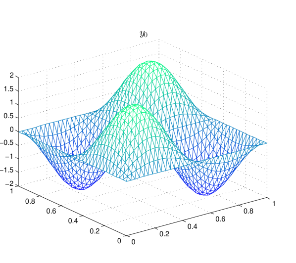
(a) $\displaystyle y_{0}$ choice A1.

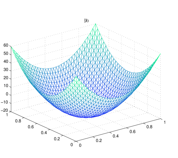
(b) $\displaystyle y_{0}$ choice A2.

Figure 1: The desired state $\displaystyle y_{0}$ choices A1 and A2.

Example 1 

In this example we define $\displaystyle\phi(s):=s^{3}$. It is easy to see that this nonlinearity satisfies Assumption 1 with $\displaystyle r=2$ and $\displaystyle M=2\sqrt{3}$. Hence, in view of Theorem 3.1 we have $\displaystyle q=4$ and a control $\displaystyle\bar{u}_{h}$ obtained from solving (3.2)-(3.5) is a global minimum if the associated adjoint state $\displaystyle\bar{p}_{h}$ satisfies

$$\|\bar{p}_{h}\|_{L^{4}(\Omega)}\leq 5^{-\frac{5}{8}}3^{\frac{3}{8}}\sqrt{2}C^{-1}_{4}\alpha^{\frac{3}{8}},$$

where $\displaystyle C^{-1}_{4}\approx 1.543145399297809$ is the constant from Lemma 6.3. For this example we consider the following three cases. Let us abbreviate

$$\eta(\alpha):=\eta(\alpha,2)=5^{-\frac{5}{8}}3^{\frac{3}{8}}\sqrt{2}C^{-1}_{4}\alpha^{\frac{3}{8}}.$$

Case 1 (unconstrained problem) In this case we set

$$\displaystyle u_{b} \displaystyle=-u_{a}=\infty,$$

$$\displaystyle y_{b} \displaystyle=-y_{a}=\infty.$$

In Table 1 we provide the values of $\displaystyle\|\bar{p}_{h}\|_{L^{4}}$, $\displaystyle\eta(\alpha)$ and $\displaystyle J(\bar{u}_{h})$ for different values of $\displaystyle\alpha$ where we consider the choice A1 for the desired state $\displaystyle y_{0}$. The findings are illustrated graphically in Figure 2. We see that for all values of $\displaystyle\alpha$ we can claim that $\displaystyle\bar{u}_{h}$ is a global minimum since $\displaystyle\|\bar{p}_{h}\|_{L^{4}}$ is less than its corresponding $\displaystyle\eta(\alpha)$. On the other hand, if we consider the choice A2 for $\displaystyle y_{0}$ we can claim $\displaystyle\bar{u}_{h}$ is a global minimum only for approximately $\displaystyle\alpha$ greater than $\displaystyle 10^{-2}$ as it can be seen from Figure 3. The numerical values are provided in Table 2.

Table 1: Example 1 Case 1 with choice A1 for $\displaystyle y_{0}$: The values of $\displaystyle\|\bar{p}_{h}\|_{L^{4}}$, $\displaystyle\eta(\alpha)$ and $\displaystyle J(\bar{u}_{h})$ for different values of $\displaystyle\alpha$.

$\displaystyle\alpha$	$\displaystyle\|\bar{p}_{h}\|_{L^{4}}$	$\displaystyle\eta(\alpha)$	$\displaystyle J(\bar{u}_{h})$
1.0e-06	9.990654861172e-05	6.776197632762e-03	3.344560044987e-03
1.0e-05	9.328604940252e-04	1.606889689070e-02	3.128947575776e-02
1.0e-04	5.916313713912e-03	3.810535956559e-02	1.967337721757e-01
1.0e-03	1.322797500856e-02	9.036204771862e-02	4.320833160546e-01
1.0e-02	1.509224717529e-02	2.142821839497e-01	4.922544738762e-01
1.0e-01	1.530600543072e-02	5.081431366100e-01	4.992144829702e-01
1.0e+00	1.532768796263e-02	1.204997272869e+00	4.999213370332e-01
1.0e+01	1.532985932323e-02	2.857498848277e+00	4.999921325890e-01
1.0e+02	1.533007649041e-02	6.776197632762e+00	4.999992132478e-01
1.0e+03	1.533009820744e-02	1.606889689070e+01	4.999999213247e-01

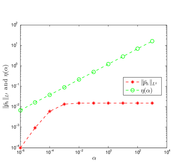
(a) $\displaystyle\|\bar{p}_{h}\|_{L^{4}}$ and $\displaystyle\eta(\alpha)$ vs. $\displaystyle\alpha$.

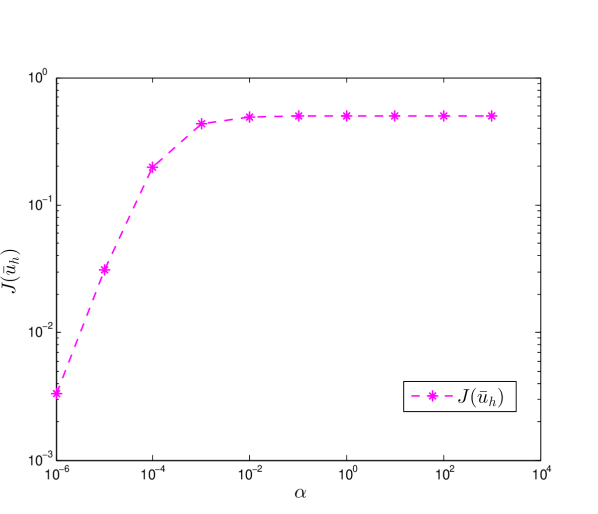
(b) $\displaystyle J(\bar{u}_{h})$ vs. $\displaystyle\alpha$.

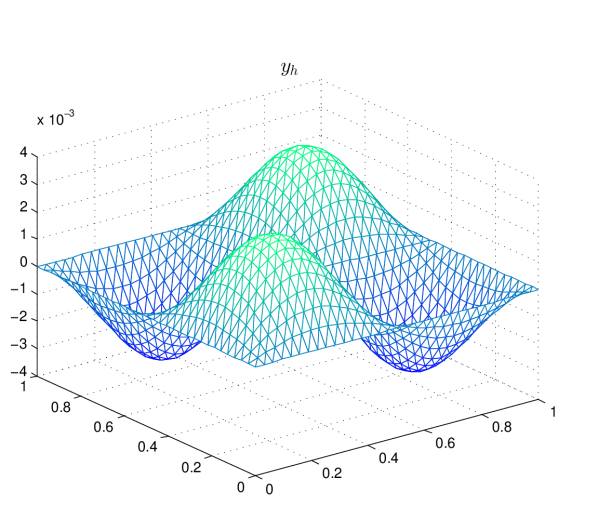
(c) The optimal state $\displaystyle\bar{y}_{h}$.

(d) The adjoint state $\displaystyle\bar{p}_{h}$.

(e) The optimal control $\displaystyle\bar{u}_{h}$.

Figure 2: Example 1 Case 1 with choice A1 for $\displaystyle y_{0}$: The values of $\displaystyle\|\bar{p}_{h}\|_{L^{4}}$, $\displaystyle\eta(\alpha)$ and $\displaystyle J(\bar{u}_{h})$ vs. $\displaystyle\alpha$. The optimal state $\displaystyle\bar{y}_{h}$, the optimal control $\displaystyle\bar{u}_{h}$ and the adjoint state $\displaystyle\bar{p}_{h}$ for $\displaystyle\alpha=10^{-1}$.

Table 2: Example 1 Case 1 with choice A2 for $\displaystyle y_{0}$: The values of $\displaystyle\|\bar{p}_{h}\|_{L^{4}}$, $\displaystyle\eta(\alpha)$ and $\displaystyle J(\bar{u}_{h})$ for different values of $\displaystyle\alpha$.

$\displaystyle\alpha$	$\displaystyle\|\bar{p}_{h}\|_{L^{4}}$	$\displaystyle\eta(\alpha)$	$\displaystyle J(\bar{u}_{h})$
1.0e-06	7.823778739727e-03	6.776197632762e-03	7.227759688190e+01
1.0e-05	2.234541300612e-02	1.606889689070e-02	1.065710637346e+02
1.0e-04	5.805844706415e-02	3.810535956559e-02	1.386316936362e+02
1.0e-03	1.125576598202e-01	9.036204771862e-02	1.568821491955e+02
1.0e-02	2.290137136719e-01	2.142821839497e-01	1.625724420922e+02
1.0e-01	2.997603240217e-01	5.081431366100e-01	1.642031427088e+02
1.0e+00	3.061090377257e-01	1.204997272869e+00	1.644198126030e+02
1.0e+01	3.066635772733e-01	2.857498848277e+00	1.644419766418e+02
1.0e+02	3.067181181971e-01	6.776197632762e+00	1.644441976184e+02
1.0e+03	3.067235630566e-01	1.606889689070e+01	1.644444197614e+02

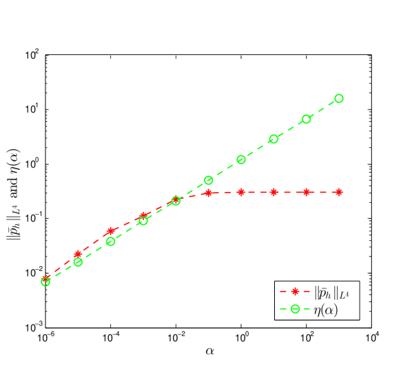
(a) $\displaystyle\|\bar{p}_{h}\|_{L^{4}}$ and $\displaystyle\eta(\alpha)$ vs. $\displaystyle\alpha$.

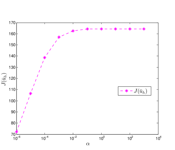
(b) $\displaystyle J(\bar{u}_{h})$ vs. $\displaystyle\alpha$.

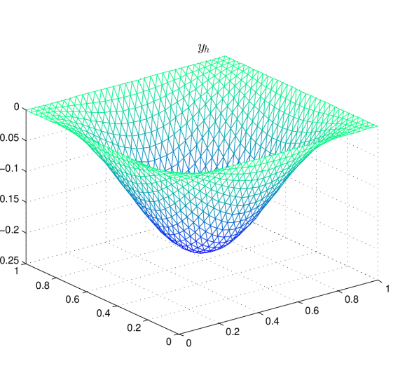
(c) The optimal state $\displaystyle\bar{y}_{h}$.

(d) The adjoint state $\displaystyle\bar{p}_{h}$.

(e) The optimal control $\displaystyle\bar{u}_{h}$.

Figure 3: Example 1 Case 1 with choice A2 for $\displaystyle y_{0}$: The values of $\displaystyle\|\bar{p}_{h}\|_{L^{4}}$, $\displaystyle\eta(\alpha)$ and $\displaystyle J(\bar{u}_{h})$ vs. $\displaystyle\alpha$. The optimal state $\displaystyle\bar{y}_{h}$, the optimal control $\displaystyle\bar{u}_{h}$ and the adjoint state $\displaystyle\bar{p}_{h}$ for $\displaystyle\alpha=10^{-1}$.

Case 2 (constrained control) In this case we consider constraints only on the control, we set

$$\displaystyle u_{a} \displaystyle=-5,$$

$$\displaystyle u_{b} \displaystyle=5,$$

$$\displaystyle y_{b} \displaystyle=-y_{a}=\infty.$$

Table 3 shows the values of $\displaystyle\|\bar{p}_{h}\|_{L^{4}}$, $\displaystyle\eta(\alpha)$ and $\displaystyle J(\bar{u}_{h})$ computed for different values of $\displaystyle\alpha$ while considering the choice A1 for $\displaystyle y_{0}$. The graphical illustration of these findings are shown in Figure 4. We see that $\displaystyle\bar{u}_{h}$ is a global minimum for $\displaystyle\alpha$ approximately greater than $\displaystyle 10^{-5}$. The numerical results associated with the choice A2 are given in Table 4 and illustrated in Figure 5. In this case $\displaystyle\bar{u}_{h}$ is a global minimum for $\displaystyle\alpha$ approximately greater than $\displaystyle 10^{-1}$.

Table 3: Example 1 Case 2 with choice A1 for $\displaystyle y_{0}$: The values of $\displaystyle\|\bar{p}_{h}\|_{L^{4}}$, $\displaystyle\eta(\alpha)$ and $\displaystyle J(\bar{u}_{h})$ for different values of $\displaystyle\alpha$.

$\displaystyle\alpha$	$\displaystyle\|\bar{p}_{h}\|_{L^{4}}$	$\displaystyle\eta(\alpha)$	$\displaystyle J(\bar{u}_{h})$
1.0e-06	1.455724773650e-02	6.776197632762e-03	4.507886038196e-01
1.0e-05	1.455724403855e-02	1.606889689070e-02	4.508916148391e-01
1.0e-04	1.455717724977e-02	3.810535956559e-02	4.519082323790e-01
1.0e-03	1.457338622672e-02	9.036204771862e-02	4.612690393001e-01
1.0e-02	1.509224717529e-02	2.142821839497e-01	4.922544738762e-01
1.0e-01	1.530600543072e-02	5.081431366100e-01	4.992144829702e-01
1.0e+00	1.532768796263e-02	1.204997272869e+00	4.999213370332e-01
1.0e+01	1.532985932323e-02	2.857498848277e+00	4.999921325890e-01
1.0e+02	1.533007649041e-02	6.776197632762e+00	4.999992132478e-01
1.0e+03	1.533009820744e-02	1.606889689070e+01	4.999999213247e-01

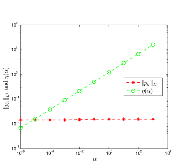
(a) $\displaystyle\|\bar{p}_{h}\|_{L^{4}}$ and $\displaystyle\eta(\alpha)$ vs. $\displaystyle\alpha$.

(b) $\displaystyle J(\bar{u}_{h})$ vs. $\displaystyle\alpha$.

(c) The optimal state $\displaystyle\bar{y}_{h}$.

(d) The adjoint state $\displaystyle\bar{p}_{h}$.

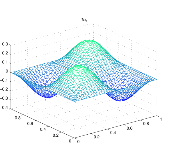
(e) The optimal control $\displaystyle\bar{u}_{h}$.

Figure 4: Example 1 Case 2 with choice A1 for $\displaystyle y_{0}$: The values of $\displaystyle\|\bar{p}_{h}\|_{L^{4}}$, $\displaystyle\eta(\alpha)$ and $\displaystyle J(\bar{u}_{h})$ vs. $\displaystyle\alpha$. The optimal state $\displaystyle\bar{y}_{h}$, the optimal control $\displaystyle\bar{u}_{h}$ and the adjoint state $\displaystyle\bar{p}_{h}$ for $\displaystyle\alpha=10^{-1}$.

Table 4: Example 1 Case 2 with choice A2 for $\displaystyle y_{0}$: The values of $\displaystyle\|\bar{p}_{h}\|_{L^{4}}$, $\displaystyle\eta(\alpha)$ and $\displaystyle J(\bar{u}_{h})$ for different values of $\displaystyle\alpha$.

$\displaystyle\alpha$	$\displaystyle\|\bar{p}_{h}\|_{L^{4}}$	$\displaystyle\eta(\alpha)$	$\displaystyle J(\bar{u}_{h})$
1.0e-06	2.954513493743e-01	6.776197632762e-03	1.636849171437e+02
1.0e-05	2.954513728927e-01	1.606889689070e-02	1.636850204333e+02
1.0e-04	2.954526968135e-01	3.810535956559e-02	1.636860509190e+02
1.0e-03	2.954464960067e-01	9.036204771862e-02	1.636961799251e+02
1.0e-02	2.955530339094e-01	2.142821839497e-01	1.637871978058e+02
1.0e-01	2.998739300063e-01	5.081431366100e-01	1.642034478360e+02
1.0e+00	3.061090377257e-01	1.204997272869e+00	1.644198126030e+02
1.0e+01	3.066635772733e-01	2.857498848277e+00	1.644419766418e+02
1.0e+02	3.067181181971e-01	6.776197632762e+00	1.644441976184e+02
1.0e+03	3.067235630566e-01	1.606889689070e+01	1.644444197614e+02

(a) $\displaystyle\|\bar{p}_{h}\|_{L^{4}}$ and $\displaystyle\eta(\alpha)$ vs. $\displaystyle\alpha$.

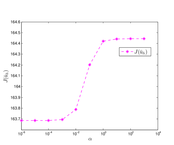
(b) $\displaystyle J(\bar{u}_{h})$ vs. $\displaystyle\alpha$.

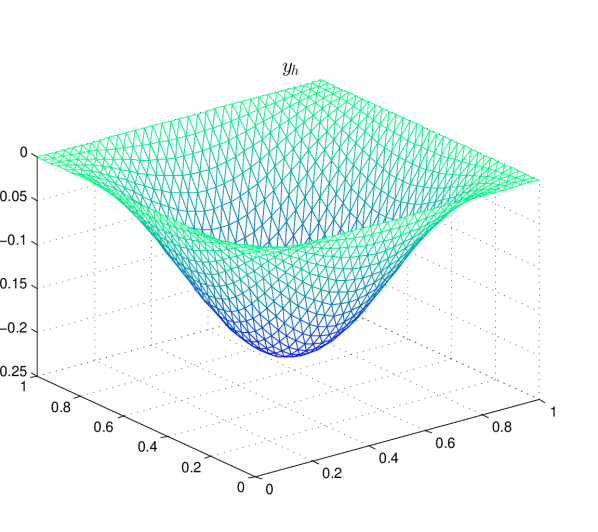
(c) The optimal state $\displaystyle\bar{y}_{h}$.

(d) The adjoint state $\displaystyle\bar{p}_{h}$.

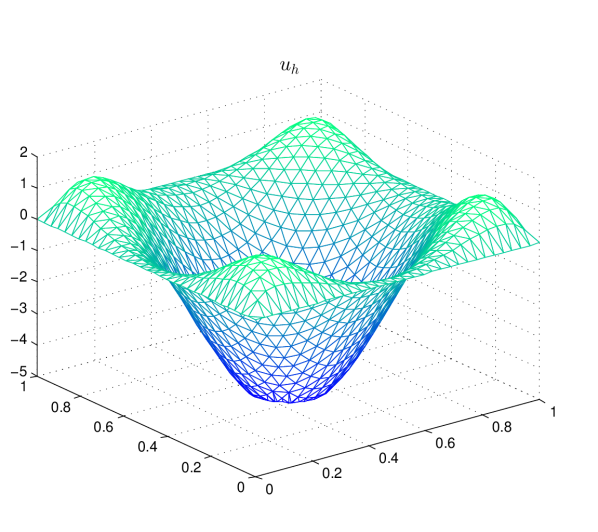
(e) The optimal control $\displaystyle\bar{u}_{h}$.

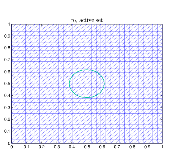
(f) The control active set ($\displaystyle\bar{u}_{h}=-5$ inside the polygonal region).

Figure 5: Example 1 Case 2 with choice A2 for $\displaystyle y_{0}$: The values of $\displaystyle\|\bar{p}_{h}\|_{L^{4}}$, $\displaystyle\eta(\alpha)$ and $\displaystyle J(\bar{u}_{h})$ vs. $\displaystyle\alpha$. The optimal state $\displaystyle\bar{y}_{h}$, the optimal control $\displaystyle\bar{u}_{h}$, the control active set and the adjoint state $\displaystyle\bar{p}_{h}$ for $\displaystyle\alpha=10^{-1}$

Case 3 (constrained state) In this case we consider constrains only on the state, we set

$$\displaystyle u_{b} \displaystyle=-u_{a}=\infty,$$

$$\displaystyle y_{a} \displaystyle=-1,$$

$$\displaystyle y_{b} \displaystyle=1.$$

The numerical findings associated with choice A1 are provided in Table 5 and illustrated in Figure 6. For the choice A2 the results are given in Table 6 and illustrated in Figure 7. In both cases we see that $\displaystyle\bar{u}_{h}$ is a global minimum for all available values of $\displaystyle\alpha$.

Table 5: Example 1 Case 3 with choice A1 for $\displaystyle y_{0}$: The values of $\displaystyle\|\bar{p}_{h}\|_{L^{4}}$, $\displaystyle\eta(\alpha)$ and $\displaystyle J(\bar{u}_{h})$ for different values of $\displaystyle\alpha$.

$\displaystyle\alpha$	$\displaystyle\|\bar{p}_{h}\|_{L^{4}}$	$\displaystyle\eta(\alpha)$	$\displaystyle J(\bar{u}_{h})$
1.0e-06	1.166321621310e-04	6.776197632762e-03	6.248613075636e-02
1.0e-05	8.045399583166e-04	1.606889689070e-02	8.942494600427e-02
1.0e-04	5.009426247692e-03	3.810535956559e-02	2.037409649052e-01
1.0e-03	1.322797500856e-02	9.036204771862e-02	4.320833160546e-01
1.0e-02	1.509224717529e-02	2.142821839497e-01	4.922544738762e-01
1.0e-01	1.530600543072e-02	5.081431366100e-01	4.992144829702e-01
1.0e+00	1.532768796263e-02	1.204997272869e+00	4.999213370332e-01
1.0e+01	1.532985932323e-02	2.857498848277e+00	4.999921325890e-01
1.0e+02	1.533007649041e-02	6.776197632762e+00	4.999992132478e-01
1.0e+03	1.533009820744e-02	1.606889689070e+01	4.999999213247e-01

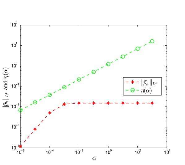
(a) $\displaystyle\|\bar{p}_{h}\|_{L^{4}}$ and $\displaystyle\eta(\alpha)$ vs. $\displaystyle\alpha$.

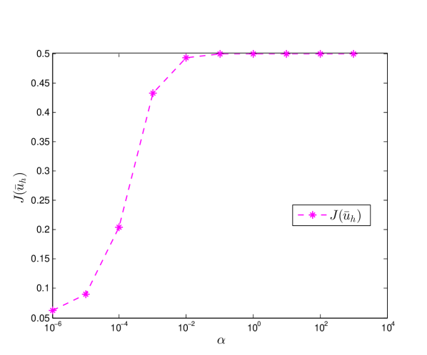
(b) $\displaystyle J(\bar{u}_{h})$ vs. $\displaystyle\alpha$.

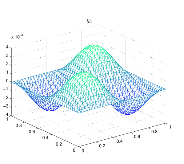
(c) The optimal state $\displaystyle\bar{y}_{h}$.

(d) The adjoint state $\displaystyle\bar{p}_{h}$.

(e) The optimal control $\displaystyle\bar{u}_{h}$.

Figure 6: Example 1 Case 3 with choice A1 for $\displaystyle y_{0}$: The values of $\displaystyle\|\bar{p}_{h}\|_{L^{4}}$, $\displaystyle\eta(\alpha)$ and $\displaystyle J(\bar{u}_{h})$ vs. $\displaystyle\alpha$. The optimal state $\displaystyle\bar{y}_{h}$, the optimal control $\displaystyle\bar{u}_{h}$ and the adjoint state $\displaystyle\bar{p}_{h}$ for $\displaystyle\alpha=10^{-1}$.

Table 6: Example 1 Case 3 with choice A2 for $\displaystyle y_{0}$: The values of $\displaystyle\|\bar{p}_{h}\|_{L^{4}}$, $\displaystyle\eta(\alpha)$ and $\displaystyle J(\bar{u}_{h})$ for different values of $\displaystyle\alpha$.

$\displaystyle\alpha$	$\displaystyle\|\bar{p}_{h}\|_{L^{4}}$	$\displaystyle\eta(\alpha)$	$\displaystyle J(\bar{u}_{h})$
1.0e-06	8.727496956489e-04	6.776197632762e-03	1.525635329141e+02
1.0e-05	6.303449080470e-03	1.606889689070e-02	1.536018906075e+02
1.0e-04	2.143214405409e-02	3.810535956559e-02	1.559131574621e+02
1.0e-03	8.541044896637e-02	9.036204771862e-02	1.600259053817e+02
1.0e-02	1.596641521237e-01	2.142821839497e-01	1.627648901943e+02
1.0e-01	2.997603240217e-01	5.081431366100e-01	1.642031427088e+02
1.0e+00	3.061090377257e-01	1.204997272869e+00	1.644198126030e+02
1.0e+01	3.066635772733e-01	2.857498848277e+00	1.644419766418e+02
1.0e+02	3.067181181971e-01	6.776197632762e+00	1.644441976184e+02
1.0e+03	3.067235630566e-01	1.606889689070e+01	1.644444197614e+02

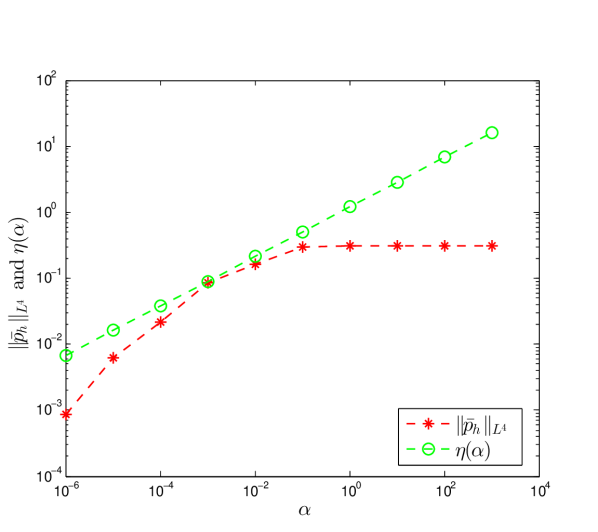
(a) $\displaystyle\|\bar{p}_{h}\|_{L^{4}}$ and $\displaystyle\eta(\alpha)$ vs. $\displaystyle\alpha$.

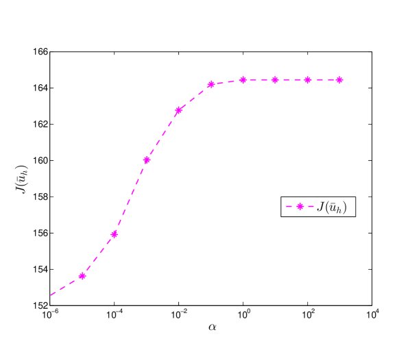
(b) $\displaystyle J(\bar{u}_{h})$ vs. $\displaystyle\alpha$.

(c) The optimal state $\displaystyle\bar{y}_{h}$.

(d) The adjoint state $\displaystyle\bar{p}_{h}$.

(e) The optimal control $\displaystyle\bar{u}_{h}$.

Figure 7: Example 1 Case 3 with choice A2 for $\displaystyle y_{0}$: The values of $\displaystyle\|\bar{p}_{h}\|_{L^{4}}$, $\displaystyle\eta(\alpha)$ and $\displaystyle J(\bar{u}_{h})$ vs. $\displaystyle\alpha$. The optimal state $\displaystyle\bar{y}_{h}$, the optimal control $\displaystyle\bar{u}_{h}$ and the adjoint state $\displaystyle\bar{p}_{h}$ for $\displaystyle\alpha=10^{-1}$.

Case 4 The following example is taken from [11, Section 7]. In particular, $\displaystyle\phi(s)=s^{3}$ and

$$\displaystyle u_{b} \displaystyle=-u_{a}=\infty,$$

$$\displaystyle y_{b} \displaystyle=\infty,$$

$$\displaystyle y_{a}(x) \displaystyle=-\frac{2}{3}+\min\bigg{(}\frac{1}{2}(x_{1}+x_{2}),\frac{1}{2}(1+x_{1}-x_{2}),\frac{1}{2}(1-x_{1}+x_{2}),1-\frac{1}{2}(x_{1}+x_{2})\bigg{)},$$

$$\displaystyle y_{0} \displaystyle=-1$$

$$\displaystyle\alpha \displaystyle=10^{-3}.$$

The numerical findings for this case are given in Table 7 and they are illustrated graphically in Figure 8. It is clear that $\displaystyle\bar{u}_{h}$ is a global minimum for the given values of $\displaystyle\alpha$.

Table 7: Example 1 Case 4: The values of $\displaystyle\|\bar{p}_{h}\|_{L^{4}}$, $\displaystyle\eta(\alpha)$ and $\displaystyle J(\bar{u}_{h})$ for different values of $\displaystyle\alpha$.

$\displaystyle\alpha$	$\displaystyle\|\bar{p}_{h}\|_{L^{4}}$	$\displaystyle\eta(\alpha)$	$\displaystyle J(\bar{u}_{h})$
1.0e-06	1.961933031441e-04	6.776197632762e-03	2.143984056211e-01
1.0e-05	7.663887131231e-04	1.606889689070e-02	2.410556714493e-01
1.0e-04	2.844056064106e-03	3.810535956559e-02	2.890783107664e-01
1.0e-03	1.055630139945e-02	9.036204771862e-02	3.690000948128e-01
1.0e-02	2.397197977885e-02	2.142821839497e-01	4.449373232494e-01
1.0e-01	4.706175447556e-02	5.081431366100e-01	4.917394785652e-01
1.0e+00	4.818113594926e-02	1.204997272869e+00	4.991551130306e-01
1.0e+01	4.829535470702e-02	2.857498848277e+00	4.999153188201e-01
1.0e+02	4.830679945384e-02	6.776197632762e+00	4.999915299530e-01
1.0e+03	4.830794415727e-02	1.606889689070e+01	4.999991529760e-01

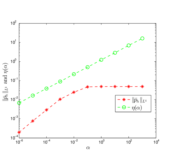
(a) $\displaystyle\|\bar{p}_{h}\|_{L^{4}}$ and $\displaystyle\eta(\alpha)$ vs. $\displaystyle\alpha$.

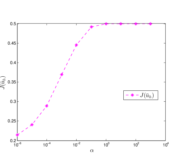
(b) $\displaystyle J(\bar{u}_{h})$ vs. $\displaystyle\alpha$.

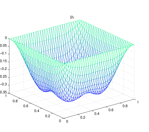
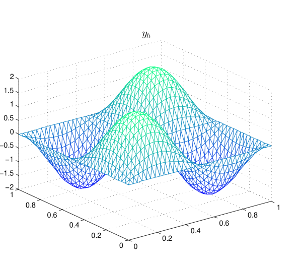
(c) The optimal state $\displaystyle\bar{y}_{h}$.

(d) The adjoint state $\displaystyle\bar{p}_{h}$.

(e) The optimal control $\displaystyle\bar{u}_{h}$.

(f) The multiplier $\displaystyle\bar{\mu}^{a}_{h}$.

Figure 8: Example 1 Case 4: The values of $\displaystyle\|\bar{p}_{h}\|_{L^{4}}$, $\displaystyle\eta(\alpha)$ and $\displaystyle J(\bar{u}_{h})$ vs. $\displaystyle\alpha$. The optimal state $\displaystyle\bar{y}_{h}$, the optimal control $\displaystyle\bar{u}_{h}$, the adjoint state $\displaystyle\bar{p}_{h}$ and the multiplier $\displaystyle\bar{\mu}^{a}_{h}$ for $\displaystyle\alpha=10^{-3}$.

Example 2 

In this example we define $\displaystyle\phi(s):=s^{5}$. We see that Assumption 1 is satisfied with

$$r=\frac{4}{3}\quad\mbox{ and }\quad M=\frac{20}{5^{\frac{3}{4}}}.$$

Hence, in view of Theorem 3.1 we have $\displaystyle q=6$ and a control $\displaystyle\bar{u}_{h}$ obtained from solving (3.2)-(3.5) is a global minimum if the associated adjoint state $\displaystyle\bar{p}_{h}$ satisfies

$$\|\bar{p}_{h}\|_{L^{6}(\Omega)}\leq\frac{11^{\frac{11}{24}}}{13^{\frac{13}{24}}2^{\frac{1}{6}}\sqrt{3}}C^{-\frac{1}{2}}_{6}\alpha^{\frac{11}{24}},$$

where $\displaystyle C^{-\frac{1}{2}}_{6}\approx 1.271251384316953$ is the constant from Lemma 6.3. For this example we consider the following three cases. We abbreviate

$$\eta(\alpha):=\eta(\alpha,\frac{4}{3})=\frac{11^{\frac{11}{24}}}{13^{\frac{13}{24}}2^{\frac{1}{6}}\sqrt{3}}C^{-\frac{1}{2}}_{6}\alpha^{\frac{11}{24}}.$$

Case 1 (unconstrained problem) In this case we set

$$\displaystyle u_{b} \displaystyle=-u_{a}=\infty,$$

$$\displaystyle y_{b} \displaystyle=-y_{a}=\infty.$$

The values of $\displaystyle\|\bar{p}_{h}\|_{L^{6}}$, $\displaystyle\eta(\alpha)$ and $\displaystyle J(\bar{u}_{h})$ for different values of $\displaystyle\alpha$ with choice A1 for $\displaystyle y_{0}$ are given in Table 8. The findings are illustrated graphically in Figure 9. We see that $\displaystyle\bar{u}_{h}$ is a global minimum for all values of $\displaystyle\alpha$ since $\displaystyle\|\bar{p}_{h}\|_{L^{6}}$ is less than its corresponding $\displaystyle\eta(\alpha)$. On the other hand, with choice A2 for $\displaystyle y_{0}$ we can claim that $\displaystyle\bar{u}_{h}$ is a global minimum only for approximately $\displaystyle\alpha$ greater than $\displaystyle 1$ as it can be seen from Figure 10. The numerical values are provided in Table 9.

Table 8: Example 2 Case 1 with choice A1 for $\displaystyle y_{0}$: The values of $\displaystyle\|\bar{p}_{h}\|_{L^{6}}$, $\displaystyle\eta(\alpha)$ and $\displaystyle J(\bar{u}_{h})$ for different values of $\displaystyle\alpha$.

$\displaystyle\alpha$	$\displaystyle\|\bar{p}_{h}\|_{L^{6}}$	$\displaystyle\eta(\alpha)$	$\displaystyle J(\bar{u}_{h})$
1.0e-06	1.179795342411e-04	8.697974773247e-04	3.663839269975e-03
1.0e-05	1.040717291260e-03	2.498914960443e-03	3.314332555914e-02
1.0e-04	6.486412414763e-03	7.179344781194e-03	1.967178952607e-01
1.0e-03	1.467650352720e-02	2.062614866979e-02	4.320253853445e-01
1.0e-02	1.672495487678e-02	5.925861229879e-02	4.922543706340e-01
1.0e-01	1.696149575588e-02	1.702490943800e-01	4.992144828609e-01
1.0e+00	1.698552077353e-02	4.891230660460e-01	4.999213370331e-01
1.0e+01	1.698792705311e-02	1.405243150394e+00	4.999921325890e-01
1.0e+02	1.698816771892e-02	4.037242258255e+00	4.999992132478e-01
1.0e+03	1.698819178587e-02	1.159893577654e+01	4.999999213247e-01

(a) $\displaystyle\|\bar{p}_{h}\|_{L^{6}}$ and $\displaystyle\eta(\alpha)$ vs. $\displaystyle\alpha$.

(b) $\displaystyle J(\bar{u}_{h})$ vs. $\displaystyle\alpha$.

(c) The optimal state $\displaystyle\bar{y}_{h}$.

(d) The adjoint state $\displaystyle\bar{p}_{h}$.

(e) The optimal control $\displaystyle\bar{u}_{h}$.

Figure 9: Example 2 Case 1 with choice A1 for $\displaystyle y_{0}$: The values of $\displaystyle\|\bar{p}_{h}\|_{L^{6}}$, $\displaystyle\eta(\alpha)$ and $\displaystyle J(\bar{u}_{h})$ vs. $\displaystyle\alpha$. The optimal state $\displaystyle\bar{y}_{h}$, the optimal control $\displaystyle\bar{u}_{h}$ and the adjoint state $\displaystyle\bar{p}_{h}$ for $\displaystyle\alpha=10^{-5}$.

Table 9: Example 2 Case 1 with choice A2 for $\displaystyle y_{0}$: The values of $\displaystyle\|\bar{p}_{h}\|_{L^{6}}$, $\displaystyle\eta(\alpha)$ and $\displaystyle J(\bar{u}_{h})$ for different values of $\displaystyle\alpha$.

$\displaystyle\alpha$	$\displaystyle\|\bar{p}_{h}\|_{L^{6}}$	$\displaystyle\eta(\alpha)$	$\displaystyle J(\bar{u}_{h})$
1.0e-06	5.510426875132e-03	8.697974773247e-04	1.185192313978e+02
1.0e-05	1.587525748968e-02	2.498914960443e-03	1.331807740335e+02
1.0e-04	4.474831409415e-02	7.179344781194e-03	1.473322027953e+02
1.0e-03	1.039480114464e-01	2.062614866979e-02	1.584387338104e+02
1.0e-02	2.428391864045e-01	5.925861229879e-02	1.626178840362e+02
1.0e-01	3.493646725426e-01	1.702490943800e-01	1.642025836782e+02
1.0e+00	3.554038724369e-01	4.891230660460e-01	1.644198119684e+02
1.0e+01	3.560155910725e-01	1.405243150394e+00	1.644419766411e+02
1.0e+02	3.560769159456e-01	4.037242258255e+00	1.644441976184e+02
1.0e+03	3.560830499750e-01	1.159893577654e+01	1.644444197614e+02

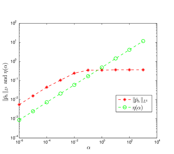
(a) $\displaystyle\|\bar{p}_{h}\|_{L^{6}}$ and $\displaystyle\eta(\alpha)$ vs. $\displaystyle\alpha$.

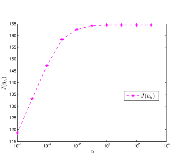
(b) $\displaystyle J(\bar{u}_{h})$ vs. $\displaystyle\alpha$.

(c) The optimal state $\displaystyle\bar{y}_{h}$.

(d) The adjoint state $\displaystyle\bar{p}_{h}$.

(e) The optimal control $\displaystyle\bar{u}_{h}$.

Figure 10: Example 2 Case 1 with choice A2 for $\displaystyle y_{0}$: The values of $\displaystyle\|\bar{p}_{h}\|_{L^{6}}$, $\displaystyle\eta(\alpha)$ and $\displaystyle J(\bar{u}_{h})$ vs. $\displaystyle\alpha$. The optimal state $\displaystyle\bar{y}_{h}$, the optimal control $\displaystyle\bar{u}_{h}$ and the adjoint state $\displaystyle\bar{p}_{h}$ for $\displaystyle\alpha=1$.

Case 2 (constrained control) In this case we consider constraints only on the control, we set

$$\displaystyle u_{a} \displaystyle=-5,$$

$$\displaystyle u_{b} \displaystyle=5,$$

$$\displaystyle y_{b} \displaystyle=-y_{a}=\infty.$$

Table 10 shows the values of $\displaystyle\|\bar{p}_{h}\|_{L^{6}}$, $\displaystyle\eta(\alpha)$ and $\displaystyle J(\bar{u}_{h})$ computed for different values of $\displaystyle\alpha$ with choice A1 for $\displaystyle y_{0}$. The graphical illustration of these findings are shown in Figure 11. We see that $\displaystyle\bar{u}_{h}$ is a global minimum for $\displaystyle\alpha$ approximately greater than $\displaystyle 10^{-3}$. The numerical results associated with the choice A2 are given in Table 11 and illustrated in Figure 12. In this case $\displaystyle\bar{u}_{h}$ is a global minimum for $\displaystyle\alpha$ approximately greater than $\displaystyle 1$.

Table 10: Example 2 Case 2 with choice A1 for $\displaystyle y_{0}$: The values of $\displaystyle\|\bar{p}_{h}\|_{L^{6}}$, $\displaystyle\eta(\alpha)$ and $\displaystyle J(\bar{u}_{h})$ for different values of $\displaystyle\alpha$.

$\displaystyle\alpha$	$\displaystyle\|\bar{p}_{h}\|_{L^{6}}$	$\displaystyle\eta(\alpha)$	$\displaystyle J(\bar{u}_{h})$
1.0e-06	1.613825290585e-02	8.697974773247e-04	4.507855415302e-01
1.0e-05	1.613824266503e-02	2.498914960443e-03	4.508885528139e-01
1.0e-04	1.613816501602e-02	7.179344781194e-03	4.519051721159e-01
1.0e-03	1.615565078678e-02	2.062614866979e-02	4.612661359991e-01
1.0e-02	1.672495487678e-02	5.925861229879e-02	4.922543706340e-01
1.0e-01	1.696149575588e-02	1.702490943800e-01	4.992144828609e-01
1.0e+00	1.698552077353e-02	4.891230660460e-01	4.999213370331e-01
1.0e+01	1.698792705311e-02	1.405243150394e+00	4.999921325890e-01
1.0e+02	1.698816771892e-02	4.037242258255e+00	4.999992132478e-01
1.0e+03	1.698819178587e-02	1.159893577654e+01	4.999999213247e-01

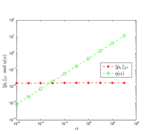
(a) $\displaystyle\|\bar{p}_{h}\|_{L^{6}}$ and $\displaystyle\eta(\alpha)$ vs. $\displaystyle\alpha$.

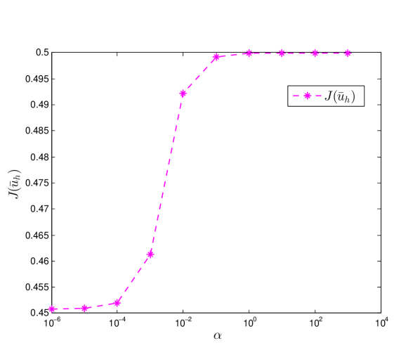
(b) $\displaystyle J(\bar{u}_{h})$ vs. $\displaystyle\alpha$.

(c) The optimal state $\displaystyle\bar{y}_{h}$.

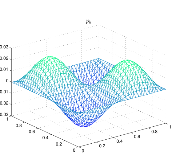
(d) The adjoint state $\displaystyle\bar{p}_{h}$.

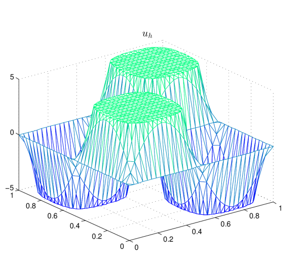
(e) The optimal control $\displaystyle\bar{u}_{h}$.

(f) The control active sets ($\displaystyle\bar{u}_{h}=5$ inside the green circles and $\displaystyle\bar{u}_{h}=-5$ inside the blue ones).

Figure 11: Example 2 Case 2 with choice A1 for $\displaystyle y_{0}$: The values of $\displaystyle\|\bar{p}_{h}\|_{L^{6}}$, $\displaystyle\eta(\alpha)$ and $\displaystyle J(\bar{u}_{h})$ vs. $\displaystyle\alpha$. The optimal state $\displaystyle\bar{y}_{h}$, the optimal control $\displaystyle\bar{u}_{h}$, the control active sets, and the adjoint state $\displaystyle\bar{p}_{h}$ for $\displaystyle\alpha=10^{-3}$.

Table 11: Example 2 Case 2 with choice A2 for $\displaystyle y_{0}$: The values of $\displaystyle\|\bar{p}_{h}\|_{L^{6}}$, $\displaystyle\eta(\alpha)$ and $\displaystyle J(\bar{u}_{h})$ for different values of $\displaystyle\alpha$.

$\displaystyle\alpha$	$\displaystyle\|\bar{p}_{h}\|_{L^{6}}$	$\displaystyle\eta(\alpha)$	$\displaystyle J(\bar{u}_{h})$
1.0e-06	3.456649663660e-01	8.697974773247e-04	1.636832040856e+02
1.0e-05	3.456649990198e-01	2.498914960443e-03	1.636833073745e+02
1.0e-04	3.456663172695e-01	7.179344781194e-03	1.636843379602e+02
1.0e-03	3.456602557101e-01	2.062614866979e-02	1.636944643396e+02
1.0e-02	3.457537810584e-01	5.925861229879e-02	1.637855203878e+02
1.0e-01	3.494672249476e-01	1.702490943800e-01	1.642029145907e+02
1.0e+00	3.554038724369e-01	4.891230660460e-01	1.644198119684e+02
1.0e+01	3.560155910725e-01	1.405243150394e+00	1.644419766411e+02
1.0e+02	3.560769159456e-01	4.037242258255e+00	1.644441976184e+02
1.0e+03	3.560830499750e-01	1.159893577654e+01	1.644444197614e+02

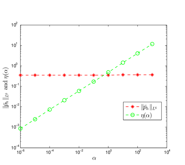
(a) $\displaystyle\|\bar{p}_{h}\|_{L^{6}}$ and $\displaystyle\eta(\alpha)$ vs. $\displaystyle\alpha$.

(b) $\displaystyle J(\bar{u}_{h})$ vs. $\displaystyle\alpha$.

(c) The optimal state $\displaystyle\bar{y}_{h}$.

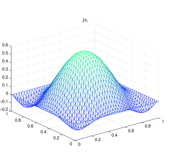
(d) The adjoint state $\displaystyle\bar{p}_{h}$.

(e) The optimal control $\displaystyle\bar{u}_{h}$.

Figure 12: Example 2 Case 2 with choice A2 for $\displaystyle y_{0}$: The values of $\displaystyle\|\bar{p}_{h}\|_{L^{6}}$, $\displaystyle\eta(\alpha)$ and $\displaystyle J(\bar{u}_{h})$ vs. $\displaystyle\alpha$. The optimal state $\displaystyle\bar{y}_{h}$, the optimal control $\displaystyle\bar{u}_{h}$ and the adjoint state $\displaystyle\bar{p}_{h}$ for $\displaystyle\alpha=1$.

Case 3 (constrained state) In this case we consider constrains only on the state, we set

$$\displaystyle u_{b} \displaystyle=-u_{a}=\infty,$$

$$\displaystyle y_{a} \displaystyle=-1,$$

$$\displaystyle y_{b} \displaystyle=1.$$

The numerical findings associated with choice A1 are provided in Table 12 and illustrated in Figure 13. We see that $\displaystyle\bar{u}_{h}$ is a global minimum for all values of $\displaystyle\alpha$. For the choice A2, the results are given in Table 13 and illustrated in Figure 14. We see that $\displaystyle\bar{u}_{h}$ is a global minimum only for $\displaystyle\alpha$ approximately greater than $\displaystyle 1$.

Table 12: Example 2 Case 3 with choice A1 for $\displaystyle y_{0}$: The values of $\displaystyle\|\bar{p}_{h}\|_{L^{6}}$, $\displaystyle\eta(\alpha)$ and $\displaystyle J(\bar{u}_{h})$ for different values of $\displaystyle\alpha$.

$\displaystyle\alpha$	$\displaystyle\|\bar{p}_{h}\|_{L^{6}}$	$\displaystyle\eta(\alpha)$	$\displaystyle J(\bar{u}_{h})$
1.0e-06	1.293594798095e-04	8.697974773247e-04	6.247856764953e-02
1.0e-05	8.673961098825e-04	2.498914960443e-03	8.936458658379e-02
1.0e-04	5.421978025542e-03	7.179344781194e-03	2.033602173575e-01
1.0e-03	1.467650352720e-02	2.062614866979e-02	4.320253853445e-01
1.0e-02	1.672495487678e-02	5.925861229879e-02	4.922543706340e-01
1.0e-01	1.696149575588e-02	1.702490943800e-01	4.992144828609e-01
1.0e+00	1.698552077353e-02	4.891230660460e-01	4.999213370331e-01
1.0e+01	1.698792705311e-02	1.405243150394e+00	4.999921325890e-01
1.0e+02	1.698816771892e-02	4.037242258255e+00	4.999992132478e-01
1.0e+03	1.698819178587e-02	1.159893577654e+01	4.999999213247e-01

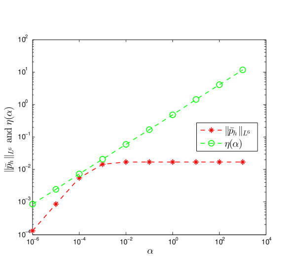
(a) $\displaystyle\|\bar{p}_{h}\|_{L^{6}}$ and $\displaystyle\eta(\alpha)$ vs. $\displaystyle\alpha$.

(b) $\displaystyle J(\bar{u}_{h})$ vs. $\displaystyle\alpha$.

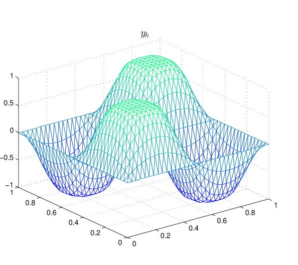
(c) The optimal state $\displaystyle\bar{y}_{h}$.

(d) The adjoint state $\displaystyle\bar{p}_{h}$.

(e) The optimal control $\displaystyle\bar{u}_{h}$.

(f) The multipliers $\displaystyle\bar{\mu}^{a}_{h}$ (in blue) and $\displaystyle\bar{\mu}^{b}_{h}$ (in green).

Figure 13: Example 2 Case 3 with choice A1 for $\displaystyle y_{0}$: The values of $\displaystyle\|\bar{p}_{h}\|_{L^{6}}$, $\displaystyle\eta(\alpha)$ and $\displaystyle J(\bar{u}_{h})$ vs. $\displaystyle\alpha$. The optimal state $\displaystyle\bar{y}_{h}$, the multipliers $\displaystyle\bar{\mu}^{a}_{h}$,$\displaystyle\bar{\mu}^{b}_{h}$, the optimal control $\displaystyle\bar{u}_{h}$ and the adjoint state $\displaystyle\bar{p}_{h}$ for $\displaystyle\alpha=10^{-5}$.

Table 13: Example 2 Case 3 with choice A2 for $\displaystyle y_{0}$: The values of $\displaystyle\|\bar{p}_{h}\|_{L^{6}}$, $\displaystyle\eta(\alpha)$ and $\displaystyle J(\bar{u}_{h})$ for different values of $\displaystyle\alpha$.

$\displaystyle\alpha$	$\displaystyle\|\bar{p}_{h}\|_{L^{6}}$	$\displaystyle\eta(\alpha)$	$\displaystyle J(\bar{u}_{h})$
1.0e-06	1.139290773221e-03	8.697974773247e-04	1.525635040951e+02
1.0e-05	8.200728224157e-03	2.498914960443e-03	1.536016384574e+02
1.0e-04	2.474482888749e-02	7.179344781194e-03	1.559116076253e+02
1.0e-03	9.716506658549e-02	2.062614866979e-02	1.600204462920e+02
1.0e-02	1.800129125912e-01	5.925861229879e-02	1.627566303073e+02
1.0e-01	3.493646725426e-01	1.702490943800e-01	1.642025836782e+02
1.0e+00	3.554038724369e-01	4.891230660460e-01	1.644198119684e+02
1.0e+01	3.560155910725e-01	1.405243150394e+00	1.644419766411e+02
1.0e+02	3.560769159456e-01	4.037242258255e+00	1.644441976184e+02
1.0e+03	3.560830499750e-01	1.159893577654e+01	1.644444197614e+02

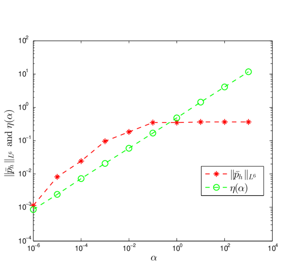
(a) $\displaystyle\|\bar{p}_{h}\|_{L^{6}}$ and $\displaystyle\eta(\alpha)$ vs. $\displaystyle\alpha$.

(b) $\displaystyle J(\bar{u}_{h})$ vs. $\displaystyle\alpha$.

(c) The optimal state $\displaystyle\bar{y}_{h}$.

(d) The adjoint state $\displaystyle\bar{p}_{h}$.

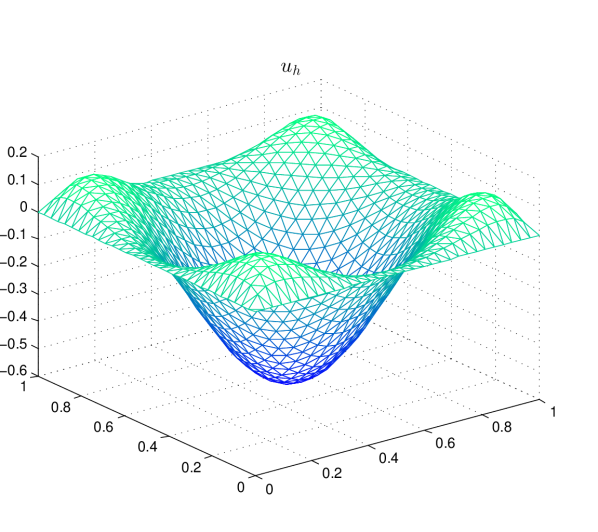
(e) The optimal control $\displaystyle\bar{u}_{h}$.

Figure 14: Example 2 Case 3 with choice A2 for $\displaystyle y_{0}$: The values of $\displaystyle\|\bar{p}_{h}\|_{L^{6}}$, $\displaystyle\eta(\alpha)$ and $\displaystyle J(\bar{u}_{h})$ vs. $\displaystyle\alpha$. The optimal state $\displaystyle\bar{y}_{h}$, the optimal control $\displaystyle\bar{u}_{h}$ and the adjoint state $\displaystyle\bar{p}_{h}$ for $\displaystyle\alpha=1$.

6 Appendix

Lemma 6.1

We have for $\displaystyle a,b\geq 0,\lambda,\mu>0$ that

$$a^{\lambda}b^{\mu}\leq\frac{\lambda^{\lambda}\mu^{\mu}}{(\lambda+\mu)^{\lambda+\mu}}(a+b)^{\lambda+\mu}.$$

Proof:.

Apply Young’s inequality $\displaystyle xy\leq\tfrac{1}{P}\,x^{P}+\tfrac{1}{Q}\,y^{Q}\,x,y\geq 0,\,\tfrac{1}{P}+\tfrac{1}{Q}=1$
to $\displaystyle P=\frac{\lambda+\mu}{\lambda}$, $\displaystyle Q=\frac{\lambda+\mu}{\mu}$ and $\displaystyle x=\bigl{(}Pa\bigr{)}^{\frac{1}{P}},\,y=\bigl{(}Qb\bigr{)}^{\frac{1}{Q}}$. ∎

Lemma 6.2

Suppose that Assumption 1 holds. Then we have for $\displaystyle a,b\in\mathbb{R}$

$$\Big{|}\int_{0}^{1}\phi^{\prime}\big{(}ta+(1-t)b\big{)}-\phi^{\prime}(b)\,dt\Big{|}\leq|a-b|L_{r}\Big{(}\int_{0}^{1}\phi^{\prime}\big{(}ta+(1-t)b\big{)}\,dt\Big{)}^{\frac{1}{r}},$$

where

$$L_{r}:=M\big{(}\frac{r-1}{2r-1}\big{)}^{\frac{r-1}{r}}.$$

Proof:.

We start by noticing that

$$\displaystyle\int_{0}^{1}\phi^{\prime}\big{(}ta+(1-t)b\big{)}-\phi^{\prime}(b)\,dt \displaystyle=\int_{0}^{1}\int_{0}^{t}\phi^{\prime\prime}\big{(}\tau a+(1-\tau)b\big{)}(a-b)\,d\tau\,dt$$

$$\displaystyle=(a-b)\int_{0}^{1}(1-t)\phi^{\prime\prime}\big{(}ta+(1-t)b\big{)}\,dt.$$

Therefore, taking the absolute value and using Assumption 1 we get

$$\displaystyle\Big{|}\int_{0}^{1}\phi^{\prime}\big{(}ta+(1-t)b\big{)}-\phi^{\prime}(b)\,dt\Big{|}\leq|a-b|M\int_{0}^{1}(1-t)\phi^{\prime}\big{(}ta+(1-t)b\big{)}^{\frac{1}{r}}\,dt$$

$$\displaystyle\leq \displaystyle|a-b|M\|1-t\|_{L^{r^{\prime}}(0,1)}\Big{(}\int_{0}^{1}\phi^{\prime}\big{(}ta+(1-t)b\big{)}\,dt\Big{)}^{\frac{1}{r}},$$

where $\displaystyle\tfrac{1}{r}+\tfrac{1}{r^{\prime}}=1$. It is easy to see that

$$\|1-t\|_{L^{r^{\prime}}(0,1)}=\big{(}\frac{1}{r^{\prime}+1}\big{)}^{\frac{1}{r^{\prime}}}=\big{(}\frac{r-1}{2r-1}\big{)}^{\frac{r-1}{r}}.$$

Denoting $\displaystyle M\|1-t\|_{L^{r^{\prime}}(0,1)}$ by $\displaystyle L_{r}$ completes the proof. ∎

Theorem 6.3

(Gagliardo–Nirenberg interpolation inequality)
For $\displaystyle 2\leq q<\infty$ we define $\displaystyle\theta=1-\frac{2}{q}$ as well as

$$GN_{q}:=\sup_{f\in H^{1}(\mathbb{R}^{2}),f\neq 0}\frac{\|f\|_{L^{q}(\mathbb{R}^{2})}}{\|f\|_{L^{2}(\mathbb{R}^{2})}^{1-\theta}\|\nabla f\|_{L^{2}(\mathbb{R}^{2})}^{\theta}}.$$

Then $\displaystyle GN_{q}\leq C_{q}:=\min(C^{(1)}_{q},C^{(2)}_{q},C^{(3)}_{q})$, where

$$\displaystyle C^{(1)}_{q} \displaystyle= \displaystyle\bigl{(}\theta C_{2,2\theta}\bigr{)}^{-\theta},\quad\mbox{ if }q\geq 4;$$ (6.1)

$$\displaystyle C^{(2)}_{q} \displaystyle= \displaystyle\frac{1}{\sqrt{\theta^{\theta}(1-\theta)^{1-\theta}}}\bigl{(}2\pi B(1,\frac{2(1-\theta)}{2\theta})\bigr{)}^{\theta/2}k_{B}(\frac{4}{2+2\theta});$$ (6.2)

$$\displaystyle C^{(3)}_{q} \displaystyle= \displaystyle\bigl{(}\frac{1}{\pi}\bigr{)}^{\frac{q-2}{2q}}\prod_{j=2}^{\infty}\bigl{(}\frac{2^{j}}{2^{j}+q-2}\bigr{)}^{\frac{2^{j}+2-q}{2^{j}q}}.$$ (6.3)

Here,

$$\displaystyle C_{2,s} \displaystyle= \displaystyle 2^{1/s}\bigl{(}\frac{2-s}{s-1}\bigr{)}^{(s-1)/s}\Bigl{(}2\pi B(\frac{2}{s},3-\frac{2}{s})\Bigr{)}^{1/2},\;1<s<2;\;C_{2,1}=2\sqrt{\pi};$$

$$\displaystyle B(a,b) \displaystyle= \displaystyle\frac{\Gamma(a)\Gamma(b)}{\Gamma(a+b)},\quad a,b>0$$

$$\displaystyle k_{B}(p) \displaystyle= \displaystyle\bigl{(}\frac{p}{2\pi}\bigr{)}^{1/p}\bigl{(}\frac{p^{\prime}}{2\pi}\bigr{)}^{-1/p^{\prime}},\quad\frac{1}{p}+\frac{1}{p^{\prime}}=1.$$

Proof:.

The bounds (6.1) and (6.2) can be found in the paper [13] by Veling. We remark that $\displaystyle GN_{q}=\lambda_{2,\theta}^{-1}$, where $\displaystyle\lambda_{2,\theta}$ is defined in [13, (1.7)]. The estimate (6.1) is [13, (1.31)] (note that $\displaystyle\theta\geq\frac{1}{2}\Leftrightarrow q\geq 4$), while (6.2) is [13, (1.42),(1.43)], where the latter bound has been proved by Nasibov in [10].
Let us now turn to the proof of (6.3). To begin, we claim that for all $\displaystyle k\in\mathbb{N}_{0}$

$$\|f\|_{L^{q}}\leq\bigl{(}\frac{1}{\pi}\bigr{)}^{\frac{1}{2}(1-\frac{q_{k}}{q})}\prod_{j=2}^{k+1}\bigl{(}\frac{2^{j}}{2^{j}+q-2}\bigr{)}^{\frac{2^{j}+2-q}{2^{j}q}}\|f\|_{L^{q_{k}}}^{\frac{q_{k}}{q}}\|\nabla f\|_{L^{2}}^{1-\frac{q_{k}}{q}},$$ (6.4)

where

$$q_{k}=2^{-k}\bigl{(}q+2(2^{k}-1)\bigr{)}.$$

The inequality clearly holds for $\displaystyle k=0$. Suppose that (6.4) is true for some $\displaystyle k\in\mathbb{N}_{0}$. We infer from Theorem 1 in [5] for the case $\displaystyle d=2$ that

$$\|f\|_{L^{2p}}\leq A\|f\|_{L^{p+1}}^{1-\theta}\|\nabla f\|_{L^{2}}^{\theta},\qquad 1<p<\infty.$$ (6.5)

Here,

$$A=\bigl{(}\frac{y(p-1)^{2}}{4\pi}\bigr{)}^{\frac{\theta}{2}}\bigl{(}\frac{2y-2}{2y}\bigr{)}^{\frac{1}{2p}}\bigl{(}\frac{\Gamma(y)}{\Gamma(y-1)}\bigr{)}^{\frac{\theta}{2}}\quad\mbox{ with }\quad\theta=\frac{2(p-1)}{4p},\quad y=\frac{p+1}{p-1}.$$

Using the formula for $\displaystyle y$ and observing that $\displaystyle\Gamma(y)=(y-1)\Gamma(y-1)$, the expression for $\displaystyle A$ can be simplified to

$$A=\bigl{(}\frac{1}{\pi}\bigr{)}^{\frac{\theta}{2}}\bigl{(}\frac{p+1}{2}\bigr{)}^{\frac{\theta}{2}-\frac{1}{2p}}.$$

We apply (6.5) for $\displaystyle p=\frac{1}{2}q_{k}$ and obtain

$$\|f\|_{L^{q_{k}}}\leq A\|f\|_{L^{\frac{1}{2}q_{k}+1}}^{1-\theta}\|\nabla f\|_{L^{2}}^{\theta},$$ (6.6)

where

$$A=\bigl{(}\frac{1}{\pi}\bigr{)}^{\frac{\theta}{2}}\bigl{(}\frac{\frac{1}{2}q_{k}+1}{2}\bigr{)}^{\frac{\theta}{2}-\frac{1}{q_{k}}}\quad\mbox{ and }\quad\theta=\frac{q_{k}-2}{2q_{k}}.$$

Since $\displaystyle\frac{1}{2}q_{k}+1=q_{k+1}$ we find that

$$A=\bigl{(}\frac{1}{\pi}\bigr{)}^{\frac{\theta}{2}}\bigl{(}\frac{q_{k+1}}{2}\bigr{)}^{\frac{\theta}{2}-\frac{1}{q_{k}}}\quad\mbox{ and }\quad\theta=1-\frac{q_{k+1}}{q_{k}},$$

which, inserted into (6.6) yields

$$\|f\|_{L^{q_{k}}}\leq\bigl{(}\frac{1}{\pi}\bigr{)}^{\frac{\theta}{2}}\bigl{(}\frac{q_{k+1}}{2}\bigr{)}^{\frac{\theta}{2}-\frac{1}{q_{k}}}\|f\|_{L^{q_{k+1}}}^{1-\theta}\|\nabla f\|^{\theta}.$$ (6.7)

Using the induction hypothesis we infer

$$\displaystyle\|f\|_{L^{q}}\leq\bigl{(}\frac{1}{\pi}\bigr{)}^{\frac{1}{2}(1-\frac{q_{k}}{q})+\frac{\theta}{2}\frac{q_{k}}{q}}\bigl{(}\frac{q_{k+1}}{2}\bigr{)}^{(\frac{\theta}{2}-\frac{1}{q_{k}})\frac{q_{k}}{q}}$$

$$\displaystyle\times\prod_{j=2}^{k+1}\bigl{(}\frac{2^{j}}{2^{j}+q-2}\bigr{)}^{\frac{2^{j}+2-q}{2^{j}q}}\|f\|_{L^{q_{k+1}}}^{(1-\theta)\frac{q_{k}}{q}}\|\nabla f\|_{L^{2}}^{1-\frac{q_{k}}{q}+\theta\frac{q_{k}}{q}}.$$

Elementary calculations show that

$$\displaystyle\frac{1}{2}\bigl{(}1-\frac{q_{k}}{q}\bigr{)}+\frac{\theta}{2}\frac{q_{k}}{q} \displaystyle= \displaystyle\frac{1}{2}\bigl{(}1-\frac{q_{k+1}}{q}\bigr{)},$$

$$\displaystyle\bigl{(}\frac{q_{k+1}}{2}\bigr{)}^{(\frac{\theta}{2}-\frac{1}{q_{k}})\frac{q_{k}}{q}} \displaystyle= \displaystyle\bigl{(}\frac{2^{k+2}}{2^{k+2}+q-2}\bigr{)}^{\frac{2^{k+2}+2-q}{2^{k+2}q}},$$

$$\displaystyle(1-\theta)\frac{q_{k}}{q} \displaystyle= \displaystyle\frac{q_{k+1}}{q},$$

$$\displaystyle 1-\frac{q_{k}}{q}+\theta\frac{q_{k}}{q} \displaystyle= \displaystyle 1-\frac{q_{k+1}}{q},$$

which implies (6.4) for $\displaystyle k+1$. The result now follows by sending $\displaystyle k\rightarrow\infty$ in (6.4) and by observing that $\displaystyle\lim_{k\rightarrow\infty}q_{k}=2$.

∎

References

- [1] N. Arada, E. Casas, and F. Tröltzsch. Error estimates for a semilinear elliptic control problem. Computational Optimization and Applications 23:201-229 (2002)
- [2] E. Casas. Error estimates for the numerical approximation of semilinear elliptic control problems with finitely many state constraints. ESAIM Control Optimisation and Calculus of Variations 8:345-374 (2002).
- [3] E. Casas and F. Tröltzsch. Second order optimality conditions and their role in PDE control. Jahresbericht der Deutschen Mathematiker-Vereinigung DOI 10.1365/s13291-014-0109-3 (2014).
- [4] K. Deckelnick and M. Hinze. A finite element approximation to elliptic control problems in the presence of control and state constraints. Hamburger Beiträge zur Angewandten Mathematik 2007-01 (2007).
- [5] M. Del Pino, J. Dolbeault. Best constants for Gagliardo-Nirenberg inequalities and applications to nonlinear diffusions. J. Math. Pures Appl. 81:847-875 (2002).
- [6] M. Hintermüller, K. Ito, and K. Kunisch. The primal-dual active set strategy as a semismooth Newton method. SIAM Journal on Optimization, 13:865-888 (2002).
- [7] M. Hinze. A variational discretization concept in control constrained optimization: The linear-quadratic case. Computational Optimization and Applications, 30:45-61 (2005).
- [8] M. Hinze and A. Rösch. Discretization of optimal control problems. International Series of Numerical Mathematics 160:391-431 (2011).
- [9] M. Hinze, R. Pinnau, M. Ulbrich, S. Ulbrich. Optimization with pde constraints. Mathematical Modelling: Theory and Applications, Volume 23, Springer (2008).
- [10] S.M. Nasibov On optimal constants in some Sobolev inequalities and their application to a nonlinear Schrödinger equation. Soviet. Math. Dokl. 40:110-115 (1990), translation of Dokl. Akad. Nauk SSSR 307:538-542 (1989).
- [11] I. Neitzel, J. Pfefferer, and A. Rösch. Finite element discretization of state-constrained elliptic optimal control problems with semilinear state equation. SIAM Journal on Control and Optimization, to appear (2015).
- [12] M. Ulbrich. Semismooth Newton methods for operator equations in function spaces. SIAM Journal on Optimization, 13(3):805–841, 2002.
- [13] E.J.M. Veling. Lower bounds for the infimum of the spectrum of the schrödinger operator in and the sobolev inequalities. JIPAM. Journal of Inequalities in Pure & Applied Mathematics [electronic only], 3, Art. 63 (2002).