Fluctuation effects on QCD phase diagram at strong coupling

Abstract:

We study the QCD phase diagram away from the strong coupling limit (SCL) with fluctuation effects in the auxiliary field Monte-Carlo (AFMC) method. First, we give an effective action which contains next-to-leading order (NLO) finite coupling effects of the strong coupling expansion as well as fluctuation effects. Second, we examine NLO effects of the strong coupling expansion in AFMC at zero quark density. We find that the chiral condensate is reduced by both NLO terms from temporal plaquettes and fluctuation effects, and almost no dependence on NLO terms from spatial plaquettes in the current analysis. These behaviors can be understood from the modification of the mass and the wave function renormalization factor by auxiliary fields as in the mean field analysis and the fluctuation effects in the strong coupling limit.

1 Introduction

Quantum Chromodynamics (QCD) phase diagram has been studied extensively, since it is related to many fields in physics — the early universe, heavy ion collisions, neutron stars and so forth. However, the structure and phase boundary of the QCD phase diagram is under debate mainly because of the notorious sign problem at finite chemical potential ($\mu$) in the lattice QCD Monte-Carlo simulations. There is a possibility that strong coupling lattice QCD (SC-LQCD) has a milder sign problem than the standard lattice QCD simulations, since the effective action can be written in terms of hadronic degrees of freedom. In SC-LQCD, the sign problem does not exist in the mean field (MF) analysis, and we could study the chiral phase transition [1, 2, 5, 6, 7, 8, 3, 4, 9]. When we include fluctuation effects, we generally have the sign problem as reported in monomer-dimer-polymer (MDP) simulation [10, 12, 11] and auxiliary filed Monte-Carlo (AFMC) method [13]. The sign problem in the strong coupling limit (SCL) is not severe in these methods, and we could investigate the QCD phase diagram even in the finite $\mu$ region.

SCL is the opposite limit of the continuum limit, so we need to include finite coupling effects to get insight into the continuum QCD phase diagram. In the MF analyses, we find that finite coupling [7, 8] and Polyakov loop effects reduce critical temperature at $\mu=0$ [9], and the critical point (the endpoint of the first order phase transition) temperature also decreases with increasing inverse coupling. On the other hand, the critical point chemical potential evolves in a different way in the cases where we include finite coupling effects of the next-to-leading order (NLO, $\mathcal{O}(1/g^{2})$) [7] and of the next-to-next-to-leading order (NNLO, $\mathcal{O}(1/g^{4})$) [8] in the MF treatment. It is necessary to include both finite coupling and fluctuation effects to study the QCD phase diagram evolution approaching to the continuum region. Both of these effects are evaluated by using reweighing method in MDP [12]. Thus it is an important step to study the QCD phase diagram from directly sampled Monte-Carlo configurations. In this paper, we construct an effective action including finite coupling effects of NLO in AFMC, and evaluate the fluctuation and finite coupling effects from the directly sampled configurations.

2 NLO SC-LQCD effective action in Auxiliary field Monte-Carlo method

In the following analysis, we only consider the case where the spatial lattice spacing $a$ is unity ($a=1$), and the color is 3 ($\mathrm{SU}(N_{c}=3)$) in 3+1 dimension $(d=3)$ spacetime. Temporal and spatial lattice sizes are indicated as $N_{\tau}$ and $L$, respectively. The lattice QCD partition function and action with one species of unrooted staggered fermion for color $\mathit{SU}(N_{c})$ in the anisotropic Euclidean spacetime are given by

$${\cal Z}_{\mathrm{LQCD}}= \int{\cal D}\left[\chi,{\bar{\chi}},U_{\nu}\right]e^{-S_{\mathrm{LQCD}}}\ ,\ S_{\mathrm{LQCD}}=S_{F}+S_{G}\ ,$$ (1)

$$S_{F}= \frac{1}{2}\sum_{x}\left[V^{+}_{x}-V^{-}_{x}\right]+\frac{1}{2\gamma}\sum_{x}\sum_{j=1}^{d}\eta_{j,x}\left[\bar{\chi}_{x}U_{j,x}\chi_{x+\hat{j}}-\bar{\chi}_{x+\hat{j}}U^{\dagger}_{j,x}\chi_{x}\right]+\frac{m_{0}}{\gamma}\sum_{x}M_{x}\ ,$$ (2)

$$V^{+}_{x}= e^{\mu/f(\gamma)}\bar{\chi}_{x}U_{0,x}\chi_{x+\hat{0}}\ ,V^{-}_{x}=e^{-\mu/f(\gamma)}\bar{\chi}_{x+\hat{0}}U^{\dagger}_{0,x}\chi_{x}\ ,M_{x}=\bar{\chi}_{x}\chi_{x}\ ,$$ (3)

$$S_{G}= \frac{2N_{c}\xi}{g_{\mathrm{\tau}}^{2}(g_{0},\xi)}\mathcal{P}_{\tau}+\frac{2N_{c}}{g_{\mathrm{s}}^{2}(g_{0},\xi)\xi}\mathcal{P}_{s}\ ,\mathcal{P}_{i}=\sum_{P_{i}}\left[1-\displaystyle\frac{1}{2N_{c}}\mathrm{Tr}\left(U_{P_{i}}+U_{P_{i}}^{\dagger}\right)\right]\ (i=\tau,s)\ ,$$ (4)

where $\chi_{x}$, $U_{\nu,x}$, $U_{P_{\tau}}$ and $U_{P_{s}}$ represent the quark field, the link variable, and the temporal and spatial plaquettes, respectively. The quark chemical potential $\mu$ is introduced in the form of the temporal component of vector potential, $\eta_{j,x}=(-1)^{x_{0}+\cdots+x_{j-1}}$ is the staggered sign factor, and $V^{\pm}_{x}$ and $M_{x}$ are mesonic composites. The temporal and spatial physical lattice spacing ratio is introduced as $f(\gamma)=a/a_{\tau}$. For simplicity, we here assume that the anisotropy parameters in the quark and gluon sectors are the same ($\gamma=\xi$), and the temporal and spatial coupling constants are also the same ($g_{\tau}=g_{s}=g$). Under these assumptions, the anisotropy is found to scale the lattice spacing ratio as $f(\gamma)=\gamma^{2}$ and we can define temperature as $T=\gamma^{2}/N_{\tau}$ from the mean field arguments in SCL [4]. We utilize this prescription in the present work. The above lattice QCD action has chiral symmetry $U(1)_{V}\times U(1)_{A}$ in the chiral limit $m_{0}\to 0$ .

We obtain an NLO effective action after the spatial link integral as follows [5, 7, 8, 4, 6, 3].

$$S_{\mathrm{eff}}^{(\mathrm{NLO})} =S_{\mathrm{eff}}^{(\mathrm{SCL})}+\Delta S_{\mathrm{}}^{(\tau)}+\Delta S_{\mathrm{}}^{(s)}+\mathcal{O}(1/\sqrt{d},1/g^{4})\ ,\$$ (5)

$$S_{\mathrm{eff}}^{(\mathrm{SCL})} =\frac{1}{2}\sum_{x}\left[V^{+}_{x}-V^{-}_{x}\right]-\displaystyle\frac{1}{4N_{c}\gamma}\sum_{x,j}M_{x}M_{x+\hat{j}}+\frac{m_{0}}{\gamma}\sum_{x}M_{x}\ ,$$ (6)

$$\Delta S_{\mathrm{}}^{(\tau)} =\frac{1}{2}C_{\tau}\sum_{x,j>0}\left[V_{x}^{+}(\mu)V_{x+\hat{j}}^{-}(\mu)+V_{x}^{+}(\mu)V_{x-\hat{j}}^{-}(\mu)\right]\ ,$$ (7)

$$\Delta S_{\mathrm{}}^{(s)} =-\frac{1}{4N_{c}\gamma^{4}}C_{s}\sum_{x,0<k<j}M_{x}M_{x+\hat{j}}M_{x+\hat{k}}M_{x+\hat{j}+\hat{k}}\ ,$$ (8)

where $C_{\tau}=1/(2N_{c}^{2}g^{2}\gamma)$ and $C_{s}=1/(2N_{c}^{3}g^{2}\gamma)$. We only consider the leading order terms of the large diminutional ($1/d$) expansion [2].

We now apply the extended Hubaard-Stratonovich transformaion  [13] in order to reduce the interaction terms of quarks into the bilinear form. As for the spatial NLO terms, we utilize sequential bosonization. First, the bosonized effective action for spatial NLO terms is given as

$$S_{\mathrm{sNLO0}}^{(\mathrm{EHS})} =\frac{L^{3}C_{s}}{8N_{c}}\sum_{\tau,\bm{u},\kappa_{u}^{j}>0,j}\kappa_{u}^{(j)}\left[|\Sigma_{\bm{u},\tau}^{(j)}|^{2}+|\Pi_{\bm{u},\tau}^{(j)}|^{2}\right]+\frac{C_{s}}{4N_{c}\gamma^{2}}\sum_{x,j}C_{j,x}^{s}M_{x}M_{x+\hat{j}}\ ,\$$ (9)

where $\kappa_{u}^{(\mathrm{j})}=\sum_{k(\neq j)}\cos u_{k}$, $\Sigma_{x}^{(j)}=\sum_{\bm{k},\kappa_{u}^{j}>0}e^{i\bm{k}\cdot\bm{x}}\tilde{\Sigma}^{(j)}_{\bm{k}}(\tau)$ , $\Pi_{x}^{(j)}=(-1)^{\tau}\sum_{\bm{k},\kappa_{u}^{j}>0}e^{i\bm{k}\cdot\bm{x}}\tilde{\Pi}^{(j)}_{\bm{k}}(\tau)$, $C_{j,x}^{s}=\sum_{k(\neq j)}\left[(\Sigma^{(j)}+i\epsilon\Pi^{(j)})_{x+\hat{k}}+(\Sigma^{(j)}+i\epsilon\Pi^{(j)})_{x-\hat{k}}\right]$, and $\epsilon_{x}=(-1)^{x_{0}+\cdots+x_{d}}$ which is related to $\gamma_{5}$ in the continuum theory. In Eq. (9), we divide the momentum region according to positive $(\kappa_{\bm{u}}^{(j)}>0)$ and negative $(\kappa_{\bm{u}}^{(j)}<0)$ modes, and use the relation $\kappa_{\bar{\bm{u}}}^{(j)}=-\kappa_{\bm{u}}^{(j)}$, where $\bar{\bm{u}}=\bm{u}+(\pi,\pi,\pi)$ as SCL [13]. Second, we use the EHS transformation to the spatial NLO action, $S_{\mathrm{sNLO0}}^{(\mathrm{EHS})}$, once again.

$$S_{\mathrm{sNLO}}^{(\mathrm{EHS})}=\frac{C_{s}}{4N_{c}}\sum_{x}\left[\phi_{x}^{2}+\varphi_{x}^{2}+i\left\{\left(\frac{M_{x}}{\gamma}+\frac{\sum_{j}C_{j,x}^{s}M_{x+\hat{j}}}{\gamma}\right)\varphi_{x}-i\left(\frac{M_{x}}{\gamma}-\frac{\sum_{j}C_{j,x}^{s}M_{x+\hat{j}}}{\gamma}\right)\phi_{x}\right\}\right]\ .$$ (10)

We also obtain the bosonized action terms of temporal NLO terms as

$$S_{\mathrm{tNLO}}^{(\mathrm{EHS})} =L^{3}C_{\tau}\sum_{\tau,\bm{k},f(\bm{k})>0}f(\bm{k})\left[|\omega_{\bm{k},\tau}|^{2}+|\Omega_{\bm{k},\tau}|^{2}\right]+\frac{1}{2}\sum_{x}\left[V_{x}^{+}(\mu)\Delta\alpha_{x}^{-}-V_{x}^{-}(\mu)\Delta\alpha_{x}^{+}\right]\ ,$$ (11)

$$\Delta\alpha_{x}^{-} =C_{\tau}\sum_{j}\left\{-i\omega_{x+\hat{j}}^{*}-i\omega_{x-\hat{j}}^{*}-(\epsilon\Omega^{*})_{x+\hat{j}}-(\epsilon\Omega^{*})_{x-\hat{j}}\right\}\ ,$$ (12)

$$\Delta\alpha_{x}^{+} =C_{\tau}\sum_{j}\left\{i\omega_{x+\hat{j}}+i\omega_{x-\hat{j}}+(\epsilon\Omega)_{x+\hat{j}}+(\epsilon\Omega)_{x-\hat{j}}\right\}\ ,$$ (13)

where $f(\bm{k})=\sum_{j}\cos k_{j}$. $\omega_{x}=\sum_{\bm{k},f(\bm{k})>0}e^{i\bm{k}\cdot\bm{x}}\tilde{\omega}_{\bm{k}}(\tau)$, $\Omega_{x}=(-1)^{\tau}\sum_{\bm{k},f(\bm{k})>0}e^{i\bm{k}\cdot\bm{x}}\tilde{\Omega}_{\bm{k}}(\tau)$. With the SCL terms [13], the total effective action after EHS is given as

$$S_{\mathrm{eff}}^{(\mathrm{EHS})} =\frac{L^{3}C_{s}}{8N_{c}}\sum_{\tau,\bm{u},\kappa_{u}^{j}>0,j}\kappa_{u}^{(j)}\left[|\Sigma_{\bm{u},\tau}^{(j)}|^{2}+|\Pi_{\bm{u},\tau}^{(j)}|^{2}\right]+L^{3}C_{\tau}\sum_{\tau,\bm{k},f(\bm{k})>0}f(\bm{k})\left[|\omega_{\bm{k},\tau}|^{2}+|\Omega_{\bm{k},\tau}|^{2}\right]$$

$$+\frac{L^{3}}{4N_{c}}\sum_{\bm{k},\tau,f(\bm{k})>0}f(\bm{k})\left[|\sigma_{\bm{k},\tau}|^{2}+|\pi_{\bm{k},\tau}|^{2}\right]+\frac{C_{s}}{4N_{c}}\sum_{x}\left[\phi_{x}^{2}+\varphi_{x}^{2}\right]$$

$$+\frac{1}{2}\sum_{x}Z_{x}\left[V_{x}^{+}(\tilde{\mu})-V_{x}^{-}(\tilde{\mu})\right]+\sum_{x}m_{x}M_{x}/\gamma\ ,$$ (14)

where $Z_{x}=\sqrt{\alpha^{+}_{x}\alpha^{-}_{x}}\ ,\ e^{\tilde{\mu}_{x}}=e^{\mu}e^{-\delta\mu_{x}}=e^{\mu}\sqrt{\alpha^{-}_{x}/\alpha^{+}_{x}}\ ,\alpha_{x}^{+}=1+\Delta\alpha_{x}^{+}\ ,\ \alpha_{x}^{-}=1+\Delta\alpha_{x}^{-}$,

$$m_{x} =m_{0}+\frac{1}{4N_{c}}\sum_{j}\left[(\sigma+i\epsilon\pi)_{x-\hat{j}}+(\sigma+i\epsilon\pi)_{x+\hat{j}}\right]+\frac{C_{s}}{4N_{c}}i\left[\left(\varphi_{x}-i\phi_{x}\right)+\sum_{j}\left(C_{j,x-\hat{j}}^{s}\varphi_{x-\hat{j}}+iC_{j,x-\hat{j}}^{s}\phi_{x-\hat{j}}\right)\right]\ .$$ (15)

It is clear that the mass and chemical potential are modified by the auxiliary fields. In the temporal kinetic terms, the wave function renormalization factor $Z_{x}$ appears as in the MF analysis [7].

Next, we integrate out Grassmann variables and temporal link variables analytically, then the effective action is written in terms of hadronic degrees of freedom as

$$S_{\mathrm{eff}}^{(\mathrm{AF})} =\frac{L^{3}C_{s}}{8N_{c}}\sum_{\tau,\bm{u},\kappa_{u}^{j}>0,j}\kappa_{u}^{(j)}\left[|\Sigma_{\bm{u}}^{(j)}|^{2}+|\Pi_{\bm{u}}^{(j)}|^{2}\right]+L^{3}C_{\tau}\sum_{\tau,\bm{k},f(\bm{k})>0}f(\bm{k})\left[|\omega_{\bm{k},\tau}|^{2}+|\Omega_{\bm{k},\tau}|^{2}\right]$$

$$+\frac{L^{3}}{4N_{c}}\sum_{\bm{k},\tau,f(\bm{k})>0}f(\bm{k})\left[|\sigma_{\bm{k},\tau}|^{2}+|\pi_{\bm{k},\tau}|^{2}\right]+\frac{C_{s}}{4N_{c}}\sum_{x}\left[\phi_{x}^{2}+\varphi_{x}^{2}\right]$$

$$-\sum_{\bm{x}}\log\left[X_{N_{\tau}}(\bm{x})^{3}-2\hat{Z}(\bm{x})^{2}X_{N_{\tau}}(\bm{x})+\hat{Z}(\bm{x})^{3}2\cosh\left(3\hat{\tilde{\mu}}(\bm{x})\right)\right]\ .$$ (16)

where $\hat{Z}(\bm{x})=\prod_{i}Z_{\bm{x},i}$ and $\hat{\tilde{\mu}}(\bm{x})=\prod_{i}\tilde{\mu}_{\bm{x},i}\$. We evaluate $X_{N_{\tau}}$ using the recursion formulae [3]. In the last step, we integrate out auxiliary fields by Monte-Carlo technique at a time. We generate Monte-Carlo configurations and investigate auxiliary field fluctuation effects in AFMC.

3 Chiral condensate in NLO with fluctuations

In order to understand the finite coupling effects from temporal and spatial plaquettes separately, we examine the phase transition at $\mu=0$ with two effective actions: one is the action in which we consider temporal NLO and SCL auxiliary fields named as t-NLO, and the other is the action in which we take account of spatial NLO and SCL terms named as sp-NLO.

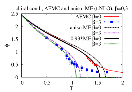
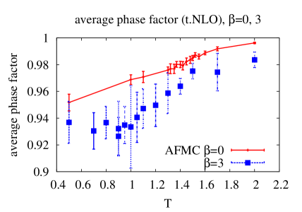
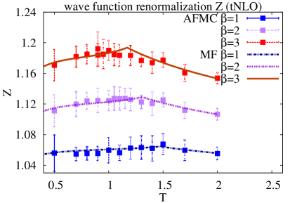
Figure 1: The chiral condensate (top left), average phase factor (top right), wave function renormalization $Z$ (bottom left), and $X_{N_{\tau}}$ (bottom right) as functions of temperature at $\mu=0$ for $\beta=2N_{c}/g^{2}=0,\ 1,\ 3$ in t-NLO. The chiral condensate in AFMC is compared with the MF results, and also with the MF results with reduced temperature, $0.93\times T$.

First, we show the chiral condensate in t-NLO at $\mu=0$ on a $4^{3}\times 4$ lattice in Fig. 1. We here regard the chiral radius as the chiral condensate. We find that the chiral condensate is reduced by both fluctuation and finite coupling effects. The main finite coupling effect is the mass reduction via the wave function renormalization factor $Z_{x}$ as discussed in MF analyses [7]. Since $Z_{x}$ coming from the temporal auxiliary fields is larger than unity as shown in Fig. 1, the effective mass $m_{x}/Z_{x}$ is suppressed, then the chiral condensate is reduced [7]. By comparison, fluctuations modify $X_{N_{\tau}}$ and play a role to enhance the apparent temperature: the chiral condensate in AFMC agrees well with the MF result at enhanced temperature, $\phi_{\mathrm{AFMC}}(T)\simeq\phi_{\mathrm{MF}}(T/0.93)$. To our surprise, fluctuation effects and finite coupling effects suppress the chiral condensate cumulatively since the both results at zero and finite $\beta$ in AFMC are well described by 93 percent scaling results in MF. In t-NLO simulation, the average phase factor is larger than 0.9 and the wight cancellation is not severe. Using the MF knowledge, the repulsive force coming from the auxiliary field, $\omega_{t}$, leads to severe sign problem. However, the field $\omega_{t}$ vanishes at zero $\mu$ and do not affect the sign problem in MF. We could expect that the average phase factor is large enough to simulate observables even in AFMC at zero $\mu$.

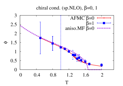
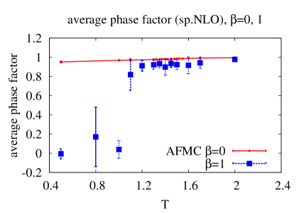
Figure 2: The chiral condensate and average phase factor as a function of temperature for $\beta=0,1$ with sp. NLO. The chiral condensate is almost the same value up to current analysis. Average phase factor is almost zero at low temperature, which means the sign problem is so severe.

In Fig. 2, we show the chiral condensate and average phase factor in sp-NLO. The chiral condensate takes almost the same value as MF results, while the average phase factor is smaller than that in t-NLO and is consistent with zero at low temperatures. We need to develop some ways to weaken the sign problem in AFMC with spatial NLO terms.

4 Summary

We have studied the fluctuation and finite coupling effects on QCD phase diagram in the framework of the strong coupling expansion and auxiliary fields Monte-Carlo (AFMC) method. We have constructed an effective action of auxiliary fields with both fluctuation and finite coupling effects. We apply the Monte-Carlo technique to integrate over auxiliary fields in order to take fluctuation effects into account. We have numerically examined the finite coupling effects from temporal and spatial plaquettes separately. When we take account of strong coupling limit (SCL) and temporal NLO auxiliary fields denoted as t-NLO, both of finite coupling and fluctuation effects are found to reduce the chiral condensate. In t-NLO simulations, we find that the average phase factor is large enough at zero chemical potential. When we consider SCL and spatial NLO auxiliary fields (sp-NLO), the chiral condensate are not modified much in the current analysis. The average phase factor is small, and it is necessary to develop a new way to weaken or avoid the sign problem in AFMC in order to obtain results in sp-NLO and full NLO simulation.

References

• [1] N. Kawamoto and J. Smit, Nucl. Phys. B192, 100 (1981); H. Kluberg-Stern, A. Morel, B. Petersson, Phys. Lett. B 114, 152 (1982); J. Hoek, N. Kawamoto, and J. Smit, Nucl. Phys. B 199, 495 (1982); P. H. Damgaard, N. Kawamoto and K. Shigemoto, Phys. Rev. Lett.  53, 2211 (1984); P. H. Damgaard, D. Hochberg, and N. Kawamoto, Phys. Lett.  B 158, 239 (1985); P. H. Damgaard, N. Kawamoto, and K. Shigemoto, Nucl. Phys. B 264, 1 (1986); V. Azcoiti, G. Di Carlo, A. Galante, and V. Laliena, J. High Energy Phys. 09, 014 (2003); K. Fukushima, Prog. Theor. Phys. Suppl.  153, 204 (2004) [hep-ph/0312057]; Y. Nishida, Phys. Rev. D 69, 094501 (2004) [hep-ph/0312371].
• [2] H. Kluberg-Stern, A. Morel, B. Petersson, Nucl. Phys. B 215 [FS7], 527 (1983);
• [3] G. Faldt and B. Petersson, Nucl. Phys. B 265, 197 (1986).
• [4] N. Bilic, K. Demeterfi and B. Petersson, Nucl. Phys. B 377, 651 (1992); N. Bilic, F. Karsch, and K. Redlich, Phys. Rev. D 45, 3228 (1992); N. Bilic and J. Cleymans, Phys. Lett. B 355, 266 (1995).
• [5] T. Jolicoeur, H. Kluberg-Stern, M. Lev, A. Morel, and B. Petersson, Nucl. Phys. B 235, 455 (1984).
• [6] I. Ichinose, Phys. Lett. B135, 148 (1984); ibid. B147, 449 (1984); I. Ichinose, Nucl. Phys. B249, 715 (1985).
• [7] K. Miura, T. Z. Nakano and A. Ohnishi, Prog. Theor. Phys.  122, 1045 (2009) [arXiv:0806.3357 [nucl-th]]; K. Miura, T. Z. Nakano, A. Ohnishi and N. Kawamoto, Phys. Rev. D 80, 074034 (2009) [arXiv:0907.4245 [hep-lat]].
• [8] T. Z. Nakano, K. Miura and A. Ohnishi, Prog. Theor. Phys.  123, 825 (2010) [arXiv:0911.3453 [hep-lat]]; T. Z. Nakano, K. Miura and A. Ohnishi, Phys. Rev. D 83, 016014 (2011) [arXiv:1009.1518 [hep-lat]].
• [9] T. Z. Nakano, K. Miura, and A. Ohnishi, Phys. Rev. D 83, 016014 (2011); T. Z. Nakano, K. Miura, and A. Ohnishi, PoS LATTICE2010, 205 (2010); K. Miura, T. Z. Nakano, A. Ohnishi, and N. Kawamoto, PoS LATTICE2011, 318 (2011) ; K. Miura, T. Z. Nakano, A. Ohnishi, and N. Kawamoto, arXiv:1106.1219 (2011).
• [10] F. Karsch and K. H. Mutter, Nucl. Phys. B 313, 541 (1989).
• [11] P. de Forcrand and M. Fromm, Phys. Rev. Lett.  104, 112005 (2010) [arXiv:0907.1915 [hep-lat]]; W. Unger and P. de Forcrand, J. Phys. G 38, 124190 (2011) [arXiv:1107.1553 [hep-lat]]; M. Fromm, Ph.D. thesis, ETH-19297, Eidgen$\mathrm{\ddot{o}}$ssische Technische Hochschule ETH Z$\mathrm{\ddot{u}}$rich, 2010; M. Fromm, P. de Forcrand, PoS LATTICE2009, 193 (2009).
• [12] P. de Forcrand, J. Langelage, O. Philipsen, and W. Unger, PoS LATTICE2013, 142 (2013) [arXiv:1312.0589 [hep-lat]]; W. Unger, Acta Phys. Polon. Supp. 7 No. 1, 127 (2014); Ph. de Forcrand, J. Langelage, O. Philipsen, and W. Unger, Phys. Rev. Lett. 113, 152002 (2014).
• [13] A. Ohnishi, T. Ichihara and T. Z. Nakano, PoS LATTICE2012, 088 (2012), T. Ichihara, T. Z. Nakano, and A. Ohnishi, PoS LATTICE2013, 143 (2013); T. Ichihara, A. Ohnishi, and T. Z. Nakano, arXiv:1401.4647.