Canonical density matrix perturbation theory

Abstract

Density matrix perturbation theory [Niklasson and Challacombe, Phys. Rev. Lett. 92, 193001 (2004)] is generalized to canonical (NVT) free energy ensembles in tight-binding, Hartree-Fock or Kohn-Sham density functional theory. The canonical density matrix perturbation theory can be used to calculate temperature dependent response properties from the coupled perturbed self-consistent field equations as in density functional perturbation theory. The method is well suited to take advantage of sparse matrix algebra to achieve linear scaling complexity in the computational cost as a function of system size for sufficiently large non-metallic materials and metals at high temperatures.

I Introduction

Materials properties such as electric conductivity, magnetic susceptibility or electrical polarizabilities, are defined from their response to perturbations that are governed by the quantum nature of the electrons. The calculation of such quantum response properties represents a major challenge because of the high cost involved. In traditional calculations the computational complexity scales cubically, ${\cal O}(N^{3})$, or worse, with the number of atoms $N$, even when effective mean field models or density functional theory are used Pople et al. (1979); Baroni et al. (2001). By using the locality of the electronic solutions it is possible to reduce the computational cost for sufficiently large, non-metallic, materials to scale only linearly, ${\cal O}(N)$, with the system size Yang (1992); Galli (1996); Ordejón (1998); Goedecker (1999); Scuseria (1999); Wu and Jayanthi (2002); Bowler and Miyazaki (2010, 2012). Initially, the development of linear scaling electronic structure theory was aimed at calculating ground state properties and not until recently has the focus shifted towards the computationally more demanding task of calculating the quantum response. A number of approaches to a quantum perturbation theory with reduced complexity have now been proposed and analyzed Yokojima and Chen (1998); Yabana and Bertsch (1999); Tsolakidis et al. (2002); Lazzeri and Mauri (2003); Ochsenfeld et al. (2004); Niklasson and Challacombe (2004); Weber et al. (2004, 2005); Niklasson and Weber (2007); Izmaylov et al. (2006); Coriani et al. (2007); Wang et al. (2007). Linear scaling quantum perturbation theory has so far mainly concerned properties at zero electronic temperature. Here we extend the idea behind linear scaling density matrix perturbation theory Niklasson and Challacombe (2004); Weber et al. (2004, 2005); Niklasson and Weber (2007) to calculations of static response properties valid also at finite electronic temperatures with fractional occupation of the states. Our proposed canonical density matrix perturbation theory, which is applicable within effective single-particle formulations, such as tight-binding, Hartree-Fock or Kohn-Sham density functional theory, can be applied to calculate temperature dependent response properties from the solution of the coupled perturbed self-consistent field equations Pople et al. (1979); Sekino and Bartlett (1986); Karna and Dupuis (1991) as in density functional perturbation theory Baroni et al. (1987, 2001). The canonical density matrix perturbation scheme should be directly applicable in a number of existing program packages for linear scaling electronic structure calculations, including CONQUEST Hernández et al. (1996); Bowler et al. (2006); Bowler and Miyazaki (2010), CP2K VandeVondele et al. (2005), ERGO Rudberg et al. (2012, 2011), FEMTECK Tsuchida and Tsukada (1998); Tsuchida (2007), FreeON Bock et al. (2008), HONPAS Qin et al. (2014), LATTE Sanville et al. (2010); Cawkwell and Niklasson (2012), ONETEP Hine et al. (2009), OPEN-MX Ozaki and Kino (2005), and SIESTA Soler et al. (2002). While originally motivated by its ability to achieve linear scaling complexity, our canonical density matrix perturbation theory is quite general and straightforward to use with high efficiency also for material systems that are too small to reach the linear scaling regime. The computational kernel of the algorithm is centered around generalized matrix-matrix multiplications that are well known to provide close to peak performance on many computer platforms using dense algebra, including graphics processing units (GPU’s) Cawkwell et al. (2012); Chow et al. (2015).

The paper is outlined as follows; first we present the canonical density matrix perturbation theory. Thereafter we show how it can be used to calculate temperature dependent free energy response properties, such as static polarizabilities and hyperpolarizabilities. We discuss the alternative of using finite difference schemes and its potential problems. We conclude by discussing the capability of the canonical density matrix perturbation theory to reach linear scaling complexity in the computational cost.

II Canonical density matrix perturbation theory

In our density matrix perturbation theory we will use the single-particle density matrix and its derivatives to represent the electronic structure and its response to perturbations. With the density matrix formulation it is easy to utilize matrix sparsity from electronic nearsightedness Kohn (1996); Goedecker (1999); Hastings (2004); Weber et al. (2005) and it allows direct calculations of observables. The effective single-particle density matrix, $P$, at the electronic temperature $T_{e}$, can be calculated from the Hamiltonian, $H$, using a recursive Fermi operator expansion Niklasson (2003, 2008); Niklasson et al. (2011); Rubensson (2012),

$$\begin{array}[]{l}{\displaystyle P=\left[e^{\beta(H-\mu I)}+I\right]^{-1}}\\ {}{}\\ {\displaystyle~{}~{}~{}\approx{\cal F}_{M}({\cal F}_{M-1}(\ldots{\cal F}_{0}(H)\ldots))},\end{array}$$ (1)

where the inverse temperature $\beta=1/(k_{B}T_{e})$, $\mu$ is the chemical potential, and $I$ is the identity matrix (see Appendix). Both $H$ and $P$ are here assumed to be matrix representations in an orthogonal basis. The expansion can be calculated through intermediate matrices $X_{n}={\cal F}_{n}(X_{n-1})$ for $n=1,2,3,\ldots,M$, where

$$\begin{array}[]{l}{\displaystyle X_{0}={\cal F}_{0}(H)=\frac{1}{2}I-2^{-(M+2)}\beta(H-\mu I),}\\ {}{}\\ {\displaystyle X_{n}={\cal F}_{n}(X_{n-1})=\frac{X_{n-1}^{2}}{X_{n-1}^{2}+(I-X_{n-1})^{2}}}.\end{array}$$ (2)

In the canonical (NVT) ensemble, the chemical potential $\mu$ is chosen such that the density matrix has the correct occupation, $Tr[P]=N_{\rm occ}$, where $N_{\rm occ}$ is the number of occupied states. The recursion scheme above provides a very efficient and rapidly converging expansion and the number of recursion steps $M$ can be kept low $(M<20)$. Because of the particular form of the Padé polynomial ${\cal F}_{n}(X_{n-1})$, each iteration involves a solution of a system of linear equations, which is well tailored for the linear conjugate gradient method Niklasson (2003, 2008); Rubensson (2012). The recursive expansion avoids the calculation of individual eigenvalues and eigenfunctions and is therefore well suited to reach linear scaling complexity in the computational cost for sufficiently large non-metallic problems, which can utilize thresholded sparse matrix algebra Goedecker (1999).

A canonical density matrix response expansion,

$$P(\lambda)=P^{(0)}+\lambda P^{(1)}+\lambda^{2}P^{(2)}+\ldots~{}~{}~{},$$ (3)

where $Tr[P^{(k)}]=0$ for $k>0$, with respect to a perturbation in the Hamiltonian,

$$H(\lambda)=H^{(0)}+\lambda H^{(1)}+\lambda^{2}H^{(2)}+\ldots,$$ (4)

can be constructed at finite electronic temperatures, $T_{e}>0$, based on the recursive Fermi operator expansion in Eqs. (1) and (2) above. The technique is given by a free energy generalization of the zero temperature linear scaling density matrix perturbation theory Niklasson and Challacombe (2004); Weber et al. (2004). The idea is to transfer the perturbations up to some specific order in each iteration step in the recursive Fermi-operator expansion, i.e.

$$X_{n}^{(k)}=\left.\frac{1}{k!}\frac{\partial^{k}}{\partial\lambda^{k}}{\cal F}_{n}(X_{n-1}^{(0)}+\lambda X_{n-1}^{(1)}+\ldots)\right\lvert_{\lambda=0},$$ (5)

for $n=0,1,\ldots,M$, where $X_{-1}^{(k)}=H^{(k)}$. The additional problem of conserving the number of particles in a canonical ensemble, which requires $Tr[P^{(k)}]=0$ for $k>0$, is achieved by including the corresponding perturbative expansion of the chemical potential, i.e.

$$\mu=\mu(\lambda)=\mu^{(0)}+\lambda\mu^{(1)}+\lambda^{2}\mu^{(2)}+\ldots~{}.$$ (6)

The values of $\mu^{(k)}$ ($k=0,1,2,\ldots$) can be found by an iterative Newton-Raphson optimization of the occupation error with respect to the chemical potential using the relation

$${\displaystyle\left.\left(\frac{1}{\lambda^{k}}\frac{\partial P}{\partial\mu^{(k)}}\right)\right\lvert_{\lambda=0}=P_{\mu}=\beta P^{(0)}(I-P^{(0)})},$$ (7)

which for the approximate expanded density matrix, Eqs. (1) and (2), is exact in the limit $M\rightarrow\infty$. The trace of $P_{\mu}$, defined here, gives the change in occupation with respect to a change in $\mu$. The small deviation from the exact analytic derivative for a finite expansion order $M$ is in practice insignificant, though for very low values of $M$ the rate of convergence will be slightly lower than quadratic in analogy to quasi Newton schemes. In combination with low temperatures, low values of $M$ may also lead to loss of convergence (see Table 2). However, in this case we could typically use regular zero temperature response theory, or alternatively, a modified search routine to adjust for the correct occupation would be needed.

The canonical density matrix perturbation theory based on Eqs. (1-7) above, which is our first key result, is summarized by Algorithm 1 for up to third order response. Each inner loop requires the solution of a system of linear equations, which can be achieved with the conjugate gradient method using $X_{n-1}^{(k)}$ as initial guesses. The linear conjugate gradient method Golub and van Loan (1996) is ideal for this purpose, since it efficiently can take advantage of matrix sparsity to reduce the scaling of the computational cost Niklasson (2003). Generalizations and modifications to higher order response, grand canonical schemes (with a fixed value of $\mu$), or spin-polarized (unrestricted) systems are straightforward. It is interesting to note that the system matrices on the left hand-side of the inner loop of Algorithm 1 are all the same, i. e. $T_{n-1}^{(0)}$. The same inverse of $T_{n-1}^{(0)}$ would therefore give the response $X^{(k)}_{n}$ for all orders $k$. The conditioning of the response algorithm should therefore be the same as for the original 0th-order expansion. The system matrix $T_{n-1}^{(0)}$ is very well conditioned with a spectral condition number smaller than or equal to 2 Rubensson (2012) at any point of the algorithm. In the limit of low temperature and high $n$, $T_{n-1}^{(0)}\rightarrow I$ and in the opposite limit of high temperatures does the condition number go to 1 as $T_{n-1}^{(0)}\rightarrow I/2$. The well behaved conditioning is independent of the condition number of the Hamiltonian used in the initialization.

Algorithm 1 Canonical density matrix response theory

  $M\leftarrow\mbox{Number of recursion steps}$

  $\mu^{(0)}\leftarrow\mbox{Initial guess}$

  $\mu^{(i)}\leftarrow 0\mbox{ Initial guess}~{}~{}\{i=1,2,3\}$

  $\beta=1/(k_{B}T_{e})\leftarrow\mbox{Choose temperature}$

  while Occupation error $>$ Tolerance do

     $X_{0}^{(0)}=\frac{1}{2}I-2^{-(2+M)}\beta(H^{(0)}-\mu^{(0)}I)$

     $X_{0}^{(i)}=-2^{-(2+M)}\beta(H^{(i)}-\mu^{(i)}I),~{}~{}\{i=1,2,3\}$

     for $n=1:M$ do

        solve for $X_{n}^{(i)},~{}~{}~{}\{i=0,1,2,3\}$

        $T_{n-1}^{(0)}X_{n}^{(0)}=C_{n-1}^{(0)}$

        $T_{n-1}^{(0)}X_{n}^{(1)}=C_{n-1}^{(1)}+B_{n-1}^{(1)}X_{n}^{(0)}$

        $T_{n-1}^{(0)}X_{n}^{(2)}=C_{n-1}^{(2)}+B_{n-1}^{(2)}X_{n}^{(0)}+B_{n-1}^{(1)}X_{n}^{(1)}$

        $T_{n-1}^{(0)}X_{n}^{(3)}=C_{n-1}^{(3)}+B_{n-1}^{(3)}X_{n}^{(0)}+B_{n-1}^{(2)}X_{n}^{(1)}+B_{n-1}^{(1)}X_{n}^{(2)}$

     end for

     $P^{(i)}=X_{M}^{(i)},~{}~{}\{i=0,1,2,3\}$

     $\mu^{(0)}=\mu^{(0)}+(N_{e}-Tr[P^{(0)}])/Tr[P_{\mu}]$

     $\mu^{(i)}=\mu^{(i)}-Tr[P^{(i)}]/Tr[P_{\mu}],~{}~{}\{i=1,2,3\}$

     ${\rm Occupation~{}error}=|Tr[P^{(0)}]-N_{e}|+\sum_{i=1}^{3}|Tr[P^{(i)}]|$

  end while

  using:

  $P_{\mu}=\beta P^{(0)}(I-P^{(0)})$

  $T_{n}^{(0)}=2X_{n}^{(0)}(X_{n}^{(0)}-I)+I$

  $C_{n}^{(m)}=\sum_{i+j=m}X_{n}^{(i)}X_{n}^{(j)},~{}~{}\{i,j\geq 0,~{}~{}m=0,1,2,3\}$

  $B_{n}^{(m)}=2(X_{n}^{(m)}-C_{n}^{(m)}),~{}~{}\{m=0,1,2,3\}$

III Free energy response theory

To study the quantum response valid at finite electronic temperatures, the electronic entropy contribution to the free energy has to be considered. We will look at two different situations: a) non self-consistent band energy response as in regular tight-binding theory using an orthogonal matrix representation and b) self-consistent free energy response as in density functional or Hartree-Fock theory using a non-orthogonal formulation. To clearly separate the two cases we will use two different notations. For the orthogonal tight-binding like formulation we keep using $H$ and $P$, which is consistent with the previous sections, and for the self-consistent free energy response we use $F$ and $D$ for the non-orthogonal matrix representations and $F^{\perp}$ and $D^{\perp}$ for the orthogonalized representations, as is explained in the sections below.

III.1 Non self-consistent tight-binding-like free energy response

In a simple tight-binding like formulation, the expansion terms for the canonical free energy,

$$\begin{array}[]{l}\Omega(\lambda)=Tr[P(\lambda)H(\lambda)]-T_{e}{\cal S}[P(\lambda)]=\\ {}\\ ~{}~{}=\Omega^{(0)}+\lambda\Omega^{(1)}+\lambda^{2}\Omega^{(2)}+\ldots,\end{array}$$ (8)

generated by a perturbation in $H(\lambda)$, Eq. (4), with the electronic entropy Parr and Yang (1989); Niklasson (2008),

$${\cal S}[P]=-k_{B}Tr[P\ln(P)+(I-P)\ln(I-P)],$$ (9)

are given by

$$\Omega^{(m)}=\frac{1}{m}\sum_{k=1}^{m}kTr[H^{(k)}P^{(m-k)}].$$ (10)

This expression, with $P^{(k)}$ calculated from our canonical density matrix perturbation scheme in Algorithm 1, is a straightforward generalization of the conventional $T_{e}=0$ limit of the “$n+1$” rule Niklasson and Weber (2007) and follows directly from the fact that the first order response term $Tr[H^{(0)}P^{(1)}]$ is cancelled by the response in the entropy Niklasson (2008). Higher-order derivatives of order $n+1$ therefore contain at most a derivative of order $n$ in the density matrix. This generalization is possible only by including the entropy term in Eq. (8), which is required to provide a variationally correct description of the energetics. We have not been able to find any explicit density matrix expressions for Wigner’s $2n+1$ rule Hyllerass (1930); Wigner (1935); McWeeny (1962); Helgaker et al. (2002); Niklasson and Challacombe (2004); Weber et al. (2005); Kussmann and Ochsenfeld (2007) that are valid also at finite temperatures. A more detailed derivation of Eq (10) is given in the appendix.

III.2 Self-consistent free energy response

In self-consistent first principles approaches such as Hartree-Fock theory McWeeny (1960) (density functional and self-consistent tight-binding theory, although different, follow equivalently) the free energy in the restricted case (without spin polarization) is given by a constrained minimization of the functional

$$\Omega_{\rm SCF}[D]=2Tr[hD]+Tr[DG(D)]-2T_{e}{\cal S}[D^{\perp}],$$ (11)

under the condition that $2Tr[DS]=N_{e}$, where $N_{e}$ is the number of electrons (two in each occupied state). Here $D^{\perp}$ is the orthogonalized representation of the Hartree-Fock density matrix $D$ such that $D=ZD^{\perp}Z^{T}$, and the orthogonalized effective single-particle Hamiltonian is given by $F^{\perp}=Z^{T}FZ$, where the Fockian $F=h+G(D)$ and $Z$ is the inverse factor of the basis set overlap matrix $S$ such that $Z^{T}SZ=I$. The density matrix, $D$, is thus given by

$$D=Z\left[e^{\beta(F^{\perp}-\mu I)}+I\right]^{-1}Z^{T},$$ (12)

which can be calculated through the recursive Fermi operator expansion in Eqs. (1) and (2). Here $h$ is the usual one-electron term and $G(D)$ is the conventional two-electron part including the Coulomb $J$ and exchange term $K$, respectively McWeeny (1960). In density functional theory, the Fockian $F$ is replaced by the corresponding Kohn-Sham Hamiltonian, where the exchange term $K$ is substituted with the exchange-correlation potential term. Notice that to make a clear distinction to the non-self-consistent response we use the notation $D$ and $F$ for the self-consistent Hartree-Fock density matrix and Fockian, i.e. the effective single-particle Hamiltonian.

With a basis-set independent first order perturbation in the one-electron term,

$$h(\lambda)=h^{(0)}+\lambda h^{(1)},$$ (13)

for example due to an external electric field, the self-consistent response in the density matrix is given by the solution of the coupled perturbed self-consistent field (SCF) equations as in density functional perturbation theory:

$$\begin{array}[]{l}{\displaystyle F(\lambda)=h^{(0)}+\lambda h^{(1)}+G(D^{(0)}+\lambda D^{(1)}+\ldots)},\\ {}{}\\ {\displaystyle F^{\perp}(\lambda)=Z^{T}F(\lambda)Z},\\ {}{}\\ {\displaystyle D(\lambda)=Z\left[e^{\beta(F^{\perp}(\lambda)-\mu I)}+I\right]^{-1}Z^{T}},\\ \end{array}$$ (14)

where $D$ and $F$ are expanded in terms of $\lambda$, i.e.

$$\begin{array}[]{l}{\displaystyle D(\lambda)=D^{(0)}+\lambda D^{(1)}+\lambda^{2}D^{(2)}+\ldots~{},}\\ {}\\ {\displaystyle F(\lambda)=F^{(0)}+\lambda F^{(1)}+\lambda^{2}F^{(2)}+\ldots~{}}.\end{array}$$ (15)

The coupled response equations above are solved in each iteration using the canonical density matrix perturbation theory as implemented in Algorithm 1 with $H$ and $P$ replaced by $F^{\perp}$ and $D^{\perp}$. At self consistency, the free energy expansion terms,

$$\Omega_{\rm SCF}(\lambda)=\Omega_{\rm SCF}[D^{(0)}]+\lambda\Omega_{\rm SCF}^{(1)}+\lambda^{2}\Omega_{\rm SCF}^{(2)}+\ldots~{}~{},$$ (16)

are given by

$$\Omega_{\rm SCF}^{(m)}=\frac{2}{m}Tr[h^{(1)}D^{(m-1)}]~{}~{}~{}m>0.$$ (17)

This simple and convenient expression for the basis-set independent free energy response, which follows (see Appendix) from Eq. (10), is another key result of this paper. The free energy response theory presented here provides a general technique to perform reduced complexity calculations of, for example, temperature-dependent static polarizabilities and hyperpolarizabilities Weber et al. (2004, 2005).

IV Finite difference approximations

An alternative to the canonical density matrix perturbation theory is to perform calculations with finite perturbations and use finite difference approximations of the free energy derivatives. However, this can be far from trivial because the numerical errors are sometimes difficult to estimate and control, in particular for high temperature hyperpolarizabilities. Nevertheless, by using finite steps $\delta\lambda$ of the perturbations in $h$, combined with multi-point high-order finite difference schemes, it is sometimes possible to reach good accuracy. This is illustrated in Fig. 1, which shows the finite difference error in the approximation of the second order free energy response, $\Omega_{\rm SCF}^{(2)}$, with respect to an external electric field for a self-consistent tight-binding model Elstner et al. (1998); Finnis et al. (1998); Frauenheim et al. (2000); Aradi et al. (2007) as implemented in the electronic structure program package LATTE Sanville et al. (2010); Cawkwell and Niklasson (2012). Finite difference calculations of higher-order hyperpolarizabilities show similar behavior.

In a finite difference approximation it is difficult to know a priori what step size $\Delta\lambda$ to use for the perturbations $\lambda h^{(1)}$ in Eq. (13). Errors may be large unless careful numerical testing is performed. This can be expensive and even when an optimal step size has been found, the computational cost is still higher than the analytical approach. For example, to calculate the second order response using the five point finite difference scheme has a computational cost of about 5 times a ground state calculation, whereas the cost for the density matrix perturbation theory is only about 3 times larger. This cost estimate does not include the additional entropy calculations. The calculation of the entropy is difficult (or impossible) to perform accurately within linear scaling complexity. Computationally favorable formulations that are based on approximate expansions of ${\cal S}[P]$ in Eq. (9) are typically poor. For example, when any of the approximate entropy expressions,

$${\cal S}_{m}[P]\approx-k_{B}\sum_{i=1}^{m}c_{i}(m)Tr[P^{m}(P-I)^{m}],$$ (18)

with the coefficients $c_{i}(m)$ in Tab. 1 are used, the relative error of the polarizability in Fig. 1 is increased by over 6 orders of magnitude for the most accurate 9 point finite difference approximation. The accuracy is at best only about 0.5 percent with any of the entropy approximations in Eq. (18) and Tab. 1. Only by avoiding explicit entropy calculations it is possible to reach a meaningful accuracy. This is possible in a finite difference approximation by using the finite differences of the dipole moments instead of the free energies. Such calculations (not shown) avoid calculating the explicit entropy term and the numerical accuracy is similar to the finite difference approximations using the free energies with the exact entropy expression as illustrated in Fig. 1.

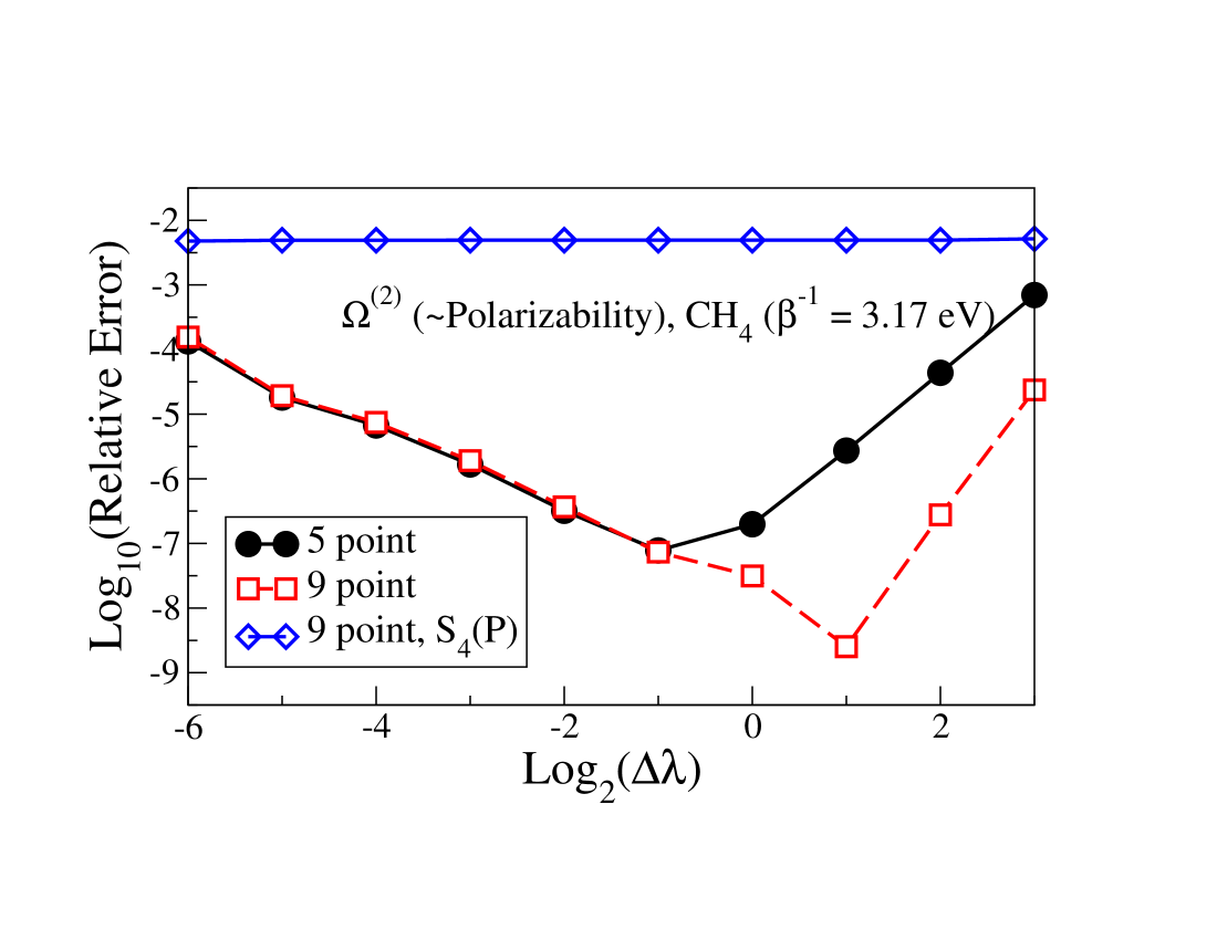
Figure 1: The relative error compared to the “exact” derivative in Eq. (17) for $\Omega_{\rm SCF}^{(2)}$ using 5 and 9 point central difference schemes for the calculation of the second order response in the free energy with respect to an external electric field, i.e. the polarizability. Either the exact entropy expression was used, Eq. (9), or the highest order ($m=4$) approximation in Eq. (18). The electronic temperature $T_{e}$ is about 37,000 K.

Table 1: Coefficients for the approximate entropy expression in Eq. (18). The coefficients are determined from the ansatz in Eq. (18) with the requirement that the function value and a few of its derivatives are correct at the midpoint 0.5 of the interval [0,1] in which $P$ has its eigenvalues.

$c_{i}(m)$	$m=1$	$m=2$	$m=4$
$c_{1}(m)$	$4\ln(2)$	$8\ln(2)-2$	$16\ln(2)-34/5$
$c_{2}(m)$		$16\ln(2)-8$	$96\ln(2)-844/15$
$c_{3}(m)$			$256\ln(2)-2336/15$
$c_{4}(m)$			$256\ln(2)-2368/15$

V first principles results

V.1 Polarizabilities and hyperpolarizabilities

Figure 2 shows the calculated temperature-dependent response for a single water molecule with respect to static electric fields. The calculations were performed with Hartree-Fock theory using the ERGO program package Rudberg et al. (2012, 2011). At lower temperatures the response values correspond to the isotropic polarizability and hyperpolarizabilities if the values are multiplied by $m!$, i. e. the factorial of the response order. At higher temperatures this interpretation is less accurate because of the limited basis set description of the thermally excited states. For relevant temperatures below 10,000 K our calculations show a very small temperature dependence, which is consistent with a fairly large HOMO-LUMO gap. For higher temperatures the errors may be significant, since the Gaussian basis set used here (cc-pVDZ) was not designed for high-temperature expansions. The calculations were performed for a single molecule in the gas phase. For periodic boundary conditions the position and the dipole moment operator are not well defined. In this case the techniques developed within the modern theory of polarizability can be applied King-SMith and Vanderbilt (1993); Resta (1994, 1998); Xiang et al. (2006).

The response properties converges quickly as a function of the number of recursion steps ($M$) in the canonical density matrix response expansion in Alg. 1, which is illustrated in Tab. 2. At higher temperatures we see a slightly slower convergence, and at low temperatures and with a small number of recursion steps there can be problems with convergence of the occupation, since the chemical potential derivative estimate $P_{\mu}=\beta P^{(0)}(I-P^{(0)})$ is less accurate. In this case we may prefer to use a regular zero-temperature response calculation.

Figure 2: (color online) The temperature dependent isotropic second-order response $\Omega_{\rm SCF}^{(2)}[\frac{1}{3}(xx+yy+zz)]=\frac{1}{3}(\Omega_{\rm SCF}^{(2)}[xx]+\Omega_{\rm SCF}^{(2)}[yy]+\Omega_{\rm SCF}^{(2)}[zz])$, and the third order and fourth order response in the $x$ direction. The canonical density matrix response Algorithm 1 for restricted Hartree-Fock theory (RHF) with a Gaussian basis set (cc-pVDZ) was used. The xyz-coordinates of the molecule: $\{{\rm O}~{}(0.0,0.0,0.0);~{}~{}{\rm H}~{}(-1.809,0.0,0.0);~{}~{}{\rm H}~{}(0.453549,1.751221,0.0)\}$ in atomic units. As a comparison and validation we show five-point finite difference calculations of the free energy derivatives. At low electronic temperatures the second-order response corresponds to $1/2$ times the isotropic polarizability (see Tab. 2).

Table 2: Convergence of the isotropic polarizability $\alpha_{\rm iso}=2\frac{1}{3}(\Omega^{(2)}_{\rm SCF}[xx]+\Omega^{(2)}_{\rm SCF}[yy]+\Omega^{(2)}_{\rm SCF}[yy])$ for three different electronic temperatures $T_{e}$ (1000 K, 30,000 K and 100,000 K) as a function of the number of recursion steps ($M$) in the canonical density matrix response expansion in Algorithm 1 for a water molecule calculated from restricted Hartree-Fock theory (RHF) with a Gaussian basis set (cc-pVDZ). The xyz-coordinates of the molecule: $\{{\rm O}~{}(0.0,0.0,0.0);~{}~{}{\rm H}~{}(-1.809,0.0,0.0);~{}~{}{\rm H}~{}(0.453549,1.751221,0.0)\}$ in atomic units. As a comparison and validation we show the $T_{e}=0$ K result of the isotropic polarizability, which was calculated by solving the linear response time-dependent Hartree-Fock (or RPA) equations Olsen et al. (1988) as implemeted in the ERGO program package Rudberg et al. (2012, 2011) applied for the zero-frequency case.

$T_{e}$ (K)	$M$	$\alpha_{\rm iso}$ (a.u.)	$T_{e}$ (K)	$M$	$\alpha_{\rm iso}$ (a.u.)	$T_{e}$ (K)	$M$	$\alpha_{\rm iso}$ (a.u.)
0 (ERGO)	n/a	-5.0112528623
1000	6	no convergence	40,000	6	-6.8540449154	100,000	6	-7.5204026148
1000	8	-5.0112527697	40,000	8	-6.8538983381	100,000	8	-7.5198385798
1000	10	-5.0112527697	40,000	10	-6.8538891617	100,000	10	-7.5198033131
1000	12	-5.0112527697	40,000	12	-6.8538885881	100,000	12	-7.5198011089
1000	14	-5.0112527697	40,000	14	-6.8538885522	100,000	14	-7.5198009711
1000	16	-5.0112527697	40,000	16	-6.8538885500	100,000	16	-7.5198009625

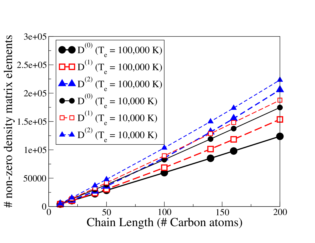
Figure 3: (color online) The sparsity scaling as a function of system size of the density matrix and its first and second order response with respect to an electric (static) dipole perturbation for two different electronic temperatures. The graphs show the number of non-zero elements of the orthogonal density matrix after a numerical threshold of 10^-5.

V.2 Linear scaling complexity

It is easy to understand the potential for a linear scaling implementation of canonical density matrix perturbation theory. Owing to nearsightedness Kohn (1996); Hastings (2004); Weber et al. (2005); Goedecker (1999), both the Hamiltonian and its perturbations, as well as the density matrix and its response, have sparse matrix representations for non-metallic materials when local basis set representations are used. The number of significant matrix elements above some small numerical threshold (or machine precision) then scales only linearly with the number of atoms for sufficiently large systems. In this case, since all operations in the canonical density matrix perturbation scheme in Algorithm 1 are based on matrix-matrix operations, the computational cost scales only linearly with system size if sparse matrix algebra is used in the calculations. This is not possible in regular Rayleigh-Schrödinger perturbation theory, which requires the calculation of individual eigenvalues and eigenfunctions. Figure 3 shows the number of non-zero elements above threshold as a function of system size for the density matrix and its first and second order response with respect to an electric dipole perturbation. The test systems are simple one-dimensional hydrocarbon chains of various lengths and the calculations where performed based on Hartree-Fock theory using a small Gaussian (STO-3G) basis. Gaussian basis sets were not designed for the high-temperature expansions demonstrated here and we can expect that the accuracy is limited. The simulations therefore only serve as a schematic demonstration of the expected behavior. For example, at higher temperatures the locality, i.e. the matrix sparsity, is increased similar to what is found for larger HOMO-LUMO gaps Goedecker (1999), and for higher order response the locality decreases, as has been seen in previous studies of the zero temperature case Weber et al. (2004, 2005). Using a larger Gaussian basis set should not change this general behavior of the locality and the results would still be uncertain. Matrix sparsity may also suffer and numerical problems may arise due to ill-conditioning from linear dependencies between many Gaussians. However, this will not affect the conditioning of the canonical density matrix response algorithm, Alg. 1, and the low spectral condition number of $T^{(0)}_{n-1}$, which is always $<2$, but it would affect the congruence transformation from the non-orthogonal atomic orbital representation of $F$ to $F^{\perp}$. The input data of the response algorithm would thus be less accurate. Localized numerical atomic orbital basis sets that have been tailored specifically for high-temperature expansions (and with low condition numbers of the overlap matrix) would then be a more appropriate choice.

VI Summary

In summary, we have presented a canonical single-particle density matrix perturbation scheme that enables the calculation of temperature dependent quantum response properties. Since our approach avoids the calculation of individual eigenvalues and eigenfunctions as well as the entropy, the theory is well adapted for reduced complexity calculations with a computational effort that scales only linearly with the system size. However, we may expect very fast parallel performance also for smaller systems in the limit of dense matrix algebra, since the computational kernel is centered around matrix-matrix multiplications that often can reach close to peak performance on modern hardware. The perturbation scheme should be applicable to a number of existing program packages for linear scaling electronic structure calculations.

VII Acknowledgement

The Los Alamos National Laboratory is operated by Los Alamos National Security, LLC for the NNSA of the US-DoE under Contract No. DE-AC52-06NA25396. We gratefully acknowledge the support of the United States Department of Energy (U.S. DOE) through LANL LDRD program, the Göran Gustafsson Foundation, the Swedish research council (grant no. 621-2012-3861), and the Swedish national strategic e-science research program (eSSENCE) as well as stimulating contributions from Travis Peery at the T-Division Ten-Bar Java Group.

VIII Appendix

VIII.1 Recursive Fermi operator expansion

There are several techniques to calculate matrix exponentials. For example, if we start with

$$e^{x}=\left(e^{x/n}\right)^{n}=\left(\frac{e^{x/(2n)}}{e^{-x/(2n)}}\right)^{n},$$ (19)

a first order Taylor expansion gives

$$e^{x}=\lim_{n\rightarrow\infty}\left(\frac{2n+x}{2n-x}\right)^{n}.$$ (20)

Using this expansion we can approximate the Fermi-Dirac distribution function, ${\Phi}(x)$, with

$${\Phi}(x)=[e^{x}+1]^{-1}=\lim_{n\rightarrow\infty}\frac{(2n-x)^{n}}{(2n+x)^{n}+(2n-x)^{n}},$$ (21)

such that

$${\Phi}(2n-4nx)\approx\frac{x^{n}}{x^{n}+(1-x)^{n}},$$ (22)

which is accurate for large values of $n$. The Padé polynomial function

$${f}_{n}(x)=\frac{x^{n}}{x^{n}+(1-x)^{n}}$$ (23)

can be expanded recursively, since

$${f}_{m\times n}(x)={f}_{m}({f}_{n}(x)).$$ (24)

This particular property enables a rapid high-order expansions in only a few iterations in the recursive Fermi-operator expansion,

$$\begin{array}[]{l}{\Phi}\left[\beta(\varepsilon_{i}-\mu)\right]={\Phi}(2n-4nx_{i})\\ {}{}\\ \approx{f}_{n}(x_{i})={f}_{2}({f}_{2}(\ldots{f}_{2}(x_{i})\ldots)),\end{array}$$ (25)

where

$$x_{i}=\frac{1}{2}-\frac{\beta}{4n}(\varepsilon_{i}-\mu)$$ (26)

with the recursion repeated $m$ times, i. e. for $n=2^{m}$. In 30 steps ($m=30$) this gives an expansion order of the Padé polynomial of over 1 billion, but often less than 10 steps are needed.

The density matrix at finite electronic temperatures,

$$P=\left[e^{\beta(H-\mu I)}+1\right]^{-1}={\Phi}\left[\beta(H-\mu I)\right],$$ (27)

can now be calculated with the recursive grand canonical Fermi operator expansion,

$$P={f}_{2}\left(\ldots f_{2}\left({f}_{2}\left(\frac{1}{2}I-2^{-(2+m)}\beta(H-\mu I)\right)\right)\ldots\right),$$ (28)

which forms the starting point in Eq. (2), with ${\cal F}_{n}(X)=f_{2}(X)$. The recursive grand canonical Fermi operator expansion, derivations, convergence analysis, and tests with various basis sets have been published previously in Refs. Niklasson (2003, 2008); Niklasson et al. (2011); Rubensson (2012).

VIII.2 Perturbation response for the non-self-consistent single particle free energy

To derive Eq. (10) we start by noting that from the definition of the density matrix response and the perturbations in the Hamiltonian, Eqs. (3) and (4), we have

$$\left.\frac{\partial^{k}}{\partial\lambda^{k}}P(\lambda)\right\lvert_{\lambda=0}=P^{[k]}=k!P^{(k)}$$ (29)

and

$$\left.\frac{\partial^{k}}{\partial\lambda^{k}}H(\lambda)\right\lvert_{\lambda=0}=H^{[k]}=k!H^{(k)},$$ (30)

where we use square brackets for the regular Taylor expansion terms, $H^{[k]}$ and $P^{[k]}$, and round brackets, $H^{(k)}$ and $P^{(k)}$, for the perturbation expansions as in Eqs. (3) and (4). Thereafter we can calculate the response terms $\Omega^{(m)}$ from the derivatives of the free energy expression in Eq. (8), i. e.

$$\Omega^{(m)}=\left.\frac{1}{m!}\frac{\partial^{m}}{\partial\lambda^{m}}\Omega(\lambda)\right\lvert_{\lambda=0}.$$ (31)

It is easy to see that the first derivative of the entropy term ${\cal S}[P(\lambda)]$ in Eq. (9) is given by

$$\begin{array}[]{l}\left.\frac{\partial}{\partial\lambda}{\cal S}[P(\lambda)]\right\lvert_{\lambda=0}=-k_{B}Tr\left[(\ln(P)-\ln(I-P))P^{[1]}\right]\\ =-k_{B}Tr\left[\ln\left(P(I-P)^{-1}\right)P^{[1]}\right]=-k_{B}Tr\left[\ln(e^{-\beta(H-\mu I)})P^{[1]}\right]\\ =k_{B}\beta Tr[HP^{(1)}],\end{array}$$ (32)

since we have a canonical perturbation $Tr[P^{[1]}]=0$ and $P=[e^{\beta(H-\mu I)}+I]^{-1}$. This means that the first order response in the free energy $\Omega(\lambda)$ is given by

$$\begin{array}[]{l}\Omega^{(1)}=\left.\frac{\partial}{\partial\lambda}\Omega(\lambda)\right\lvert_{\lambda=0}=Tr[H^{(1)}P^{(0)}]+Tr[H^{(0)}P^{(1)}]-T_{e}k_{B}\beta Tr[HP^{(1)}]\\ =Tr[H^{[1]}P^{[0]}]=Tr[H^{(1)}P^{(0)}].\end{array}$$ (33)

For the second order expansion we find that

$$\begin{array}[]{l}\Omega^{(2)}=\frac{1}{2}Tr[H^{[1]}P^{[1]}+H^{[2]}P^{[0]}]\\ =\frac{1}{2}\left(Tr[H^{(1)}P^{(1)}]+2Tr[H^{(2)}P^{(0)}]\right).\end{array}$$ (34)

For the third order expansion we find that

$$\begin{array}[]{l}\Omega^{(3)}=\frac{1}{6}Tr[H^{[1]}P^{[2]}+H^{[2]}P^{[1]}+H^{[3]}P^{[0]}+H^{[2]}P^{[1]}]\\ =\frac{1}{6}Tr[2H^{(1)}P^{(2)}+2H^{(2)}P^{(1)}+6H^{(3)}P^{(0)}+2H^{(2)}P^{(1)}]\\ =\frac{1}{3}\left(Tr[H^{(1)}P^{(2)}]+2Tr[H^{(2)}P^{(1)}]+3Tr[H^{(3)}P^{(0)}]\right).\end{array}$$ (35)

The straightforward $m$th-order generalization from consecutive derivatives gives Eq. (10).

VIII.3 Basis-set independent self-consistent free energy response

To derive the basis-set independent response of the free energy in Eq. (17) we first calculate the first order derivative of

$$\Omega_{\rm SCF}[D]=2Tr[hD]+Tr[DG(D)]-2T_{e}{\cal S}[D^{\perp}],$$ (36)

with respect to $\lambda$ in Eq. (13), i. e.

$$\begin{array}[]{l}\left.\frac{\partial}{\partial\lambda}\Omega_{\rm SCF}[D]\right\lvert_{\lambda=0}\\ =2Tr[h^{(1)}D+hD^{[1]}]+2Tr[D^{[1]}G(D)]-2T_{e}k_{B}\beta Tr[F^{\perp}{D^{\perp}}^{[1]}]\\ =2Tr[h^{(1)}D]+2Tr[(h+G(D))D^{[1]}]-2Tr[F^{\perp}{D^{\perp}}^{[1]}]\\ =2Tr[h^{(1)}D^{[0]}]+2Tr[FD^{[1]}]-2Tr[Z^{T}FZ{D^{\perp}}^{[1]}]\\ =2Tr[h^{(1)}D^{[0]}]+2Tr[FD^{[1]}]-2Tr[FD^{[1]}]=2Tr[h^{(1)}D^{[0]}]\end{array}$$ (37)

where we have derived the entropy derivative as in Eq. (32) above, used the definition of the Fockian, $F=h+G(D)$, applied the congruence transformation between the orthogonal and non-orthogonal representations, e. g. $F^{\perp}=Z^{T}FZ$, and the cyclic permutation under the trace. Subsequent derivatives, analogous to the previous Appendix subsection above, gives Eq. (17).

References

- Pople et al. (1979) J. Pople, R. Krishnan, H. B. Schlegel, and J. S. Binkley, Int. J. Quantum Chem. Symp. S13, 225 (1979).
- Baroni et al. (2001) S. Baroni, S. de Gironcoli, A. D. Corso, and P. Giannozzi, Rev. Mod. Phys. 73, 515 (2001).
- Yang (1992) W. Yang, Phys. Rev. Lett. 66, 1438 (1992).
- Galli (1996) G. Galli, Cur. Op. Sol. State Mat. Sci. 1, 864 (1996).
- Ordejón (1998) P. Ordejón, Comput. Mater. Sci. 12, 157 (1998).
- Goedecker (1999) S. Goedecker, Rev. Mod. Phys. 71, 1085 (1999).
- Scuseria (1999) G. Scuseria, J. Phys. Chem. 103, 4782 (1999).
- Wu and Jayanthi (2002) S. Y. Wu and C. S. Jayanthi, Phys. Rep. 358, 1 (2002).
- Bowler and Miyazaki (2010) D. R. Bowler and T. Miyazaki, J. Phys. Condens: Matter 22, 074207 (2010).
- Bowler and Miyazaki (2012) D. R. Bowler and T. Miyazaki, Rep. Prog. Phys. 75, 036503 (2012).
- Yokojima and Chen (1998) S. Yokojima and G. H. Chen, Chem. Phys. Lett. 292, 379 (1998).
- Yabana and Bertsch (1999) K. Yabana and G. F. Bertsch, Int. J. Quantum Chem. 75, 55 (1999).
- Tsolakidis et al. (2002) A. Tsolakidis, D. Sanches-Portal, and R. Martin, Phys. Rev. B 66, 235416 (2002).
- Lazzeri and Mauri (2003) M. Lazzeri and F. Mauri, Phys. Rev. Lett. 90, 36401 (2003).
- Ochsenfeld et al. (2004) C. Ochsenfeld, J. Kussmann, and F. Koziol, Angewandte Chemie 43, 4485 (2004).
- Niklasson and Challacombe (2004) A. M. N. Niklasson and M. Challacombe, Phys. Rev. Lett. 92, 193001 (2004).
- Weber et al. (2004) V. Weber, A. M. N. Niklasson, and M. Challacombe, Phys. Rev. Lett. 92, 193002 (2004).
- Weber et al. (2005) V. Weber, A. M. N. Niklasson, and M. Challacombe, J. Chem. Phys. 123, 44106 (2005).
- Niklasson and Weber (2007) A. M. N. Niklasson and V. Weber, J. Chem. Phys. 127, 064105 (2007).
- Izmaylov et al. (2006) A. F. Izmaylov, E. N. Brothers, and G. E. Scuseria, J. Chem. Phys. 125, 224105 (2006).
- Coriani et al. (2007) S. Coriani, S. Host, B. Jasnik, L. Thogersen, J. Olsen, P. Jorgensen, S. Reine, F. Pawlowski, T. Helgaker, and P. Salek, J. Chem. Phys. 126, 154108 (2007).
- Wang et al. (2007) F. Wang, C. Y. Yam, G. H. Chen, and K. Fan, J. Chem. Phys. 126, 134104 (2007).
- Sekino and Bartlett (1986) H. Sekino and R. J. Bartlett, J. Chem. Phys. 85, 976 (1986).
- Karna and Dupuis (1991) S. P. Karna and M. Dupuis, J. Comput. Chem. 12, 487 (1991).
- Baroni et al. (1987) S. Baroni, P. Giannozzi, and A. Testa, Phys. Rev. Lett. 58, 1861 (1987).
- Hernández et al. (1996) E. Hernández, M. J. Gillan, and C. Goringe, Phys. Rev. B 53, 7147 (1996).
- Bowler et al. (2006) D. R. Bowler, R. Choudhury, M. J. Gillan, and T. Miyazaki, Phys. Stat. Sol. B 243, 898 (2006).
- Sanville et al. (2010) E. Sanville, N. Bock, A. Niklasson, M. Cawkwell, T. Sewell, D. Dattelbaum, and S. Sheffield, 14th International Detonation Symposium p. 98667 (2010).
- Cawkwell and Niklasson (2012) M. J. Cawkwell and A. M. N. Niklasson, J. Chem. Phys. 137, 134105 (2012).
- Tsuchida and Tsukada (1998) E. Tsuchida and M. Tsukada, J. Phys. Soc. Jpn 67, 3844 (1998).
- Tsuchida (2007) E. Tsuchida, J. Phys. Soc. Jpn 76, 034708 (2007).
- Bock et al. (2008) N. Bock, M. Challacombe, C. K. Gan, G. Henkelman, K. Nemeth, A. M. N. Niklasson, A. Odell, E. Schwegler, C. J. Tymczak, and V. Weber, FreeON (2008), Los Alamos National Laboratory (LA-CC 01-2; LA- CC-04-086), Copyright University of California., URL http://www.nongnu.org/freeon/.
- VandeVondele et al. (2005) J. VandeVondele, M. Krack, F. Mohamed, M. Parrinello, T. Chassaing, and J. Hutter, Comput. Phys. Comm. 167, 103 (2005).
- Qin et al. (2014) X. Qin, H. Shang, H. Xiang, Z. Li, and J. Yang, Int. J. Quantum Chem. p. 1 (2014).
- Olsen et al. (1988) J. Olsen, H. J. Aa. Jensen, and P. Jorgensen, J. Comput. Phys. 74, 265 (1988).
- Rudberg et al. (2012) E. Rudberg, E. H. Rubensson, and P. Sałek, Ergo (version 3.51); a quantum chemistry program for large scale self-consistent field calculations (2012), URL http://www.ergoscf.org.
- Rudberg et al. (2011) E. Rudberg, E. H. Rubensson, and P. Sałek, J. Chem. Theory Comput. 7, 340 (2011).
- Ozaki and Kino (2005) T. Ozaki and H. Kino, Phys. Rev. B 72, 045121 (2005).
- Hine et al. (2009) N. D. Hine, P. D. Haynes, A. A. Mostofi, C.-K. Skylaris, and M. C. Payne, Comput. Phys. Comm. 180, 1041 (2009).
- Soler et al. (2002) J. M. Soler, E. Artacho, J. D. Gale, A. Garcia, J. Junquera, P. Ordejon, and D. Sanchez-Portal, J. Phys.: Condens. Matter 14, 2745 (2002).
- Cawkwell et al. (2012) M. J. Cawkwell, E. J. Sanville, S. M. Mniszewski, and A. M. N. Niklasson, J. Chem. Theory Comput. 8, 4094 (2012).
- Chow et al. (2015) E. Chow, X. Liu, M. Smelyanskiy, and J. R. Hammond, J. Chem. Phys. 142, 104103 (2015).
- Kohn (1996) W. Kohn, Phys. Rev. Lett. 76, 3168 (1996).
- Hastings (2004) M. B. Hastings, Phys. Rev. Lett. 93, 126402 (2004).
- Niklasson (2003) A. M. N. Niklasson, Phys. Rev. B 68, 233104 (2003).
- Niklasson (2008) A. M. N. Niklasson, J. Chem. Phys. 129, 244107 (2008).
- Niklasson et al. (2011) A. M. N. Niklasson, P. Steneteg, and N. Bock, J. Chem. Phys. 135, 164111 (2011).
- Rubensson (2012) E. H. Rubensson, SIAM J. Sci. Comput. 34, B1 (2012).
- Golub and van Loan (1996) G. Golub and C. F. van Loan, Matrix Computations (Johns Hopkins University Press, Baltimore, 1996).
- Parr and Yang (1989) R. G. Parr and W. Yang, Density-functional theory of atoms and molecules (Oxford University Press, Oxford, 1989).
- Hyllerass (1930) E. Hyllerass, Z. Phys. 65, 209 (1930).
- Wigner (1935) E. Wigner, Math. Natur. Anz. 53, 477 (1935).
- McWeeny (1962) R. McWeeny, Phys. Rev. 126, 1028 (1962).
- Helgaker et al. (2002) T. Helgaker, P. Jorgensen, and J. Olsen, Molecular Electronic-Structure Theory (John Wiley and Sons Ltd, New York, 2002), 1st ed.
- Kussmann and Ochsenfeld (2007) J. Kussmann and C. Ochsenfeld, J. Chem. Phys. 127, 204103 (2007).
- McWeeny (1960) R. McWeeny, Rev. Mod. Phys. 32, 335 (1960).
- Elstner et al. (1998) M. Elstner, D. Poresag, G. Jungnickel, J. Elstner, M. Haugk, T. Frauenheim, S. Suhai, and G. Seifert, Phys. Rev. B 58, 7260 (1998).
- Finnis et al. (1998) M. W. Finnis, A. T. Paxton, M. Methfessel, and M. van Schilfgarde, Phys. Rev. Lett. 81, 5149 (1998).
- Frauenheim et al. (2000) T. Frauenheim, G. Seifert, M. E. aand Z. Hajnal, G. Jungnickel, D. Poresag, S. Suhai, and R. Scholz, Phys. Stat. sol. 217, 41 (2000).
- Aradi et al. (2007) B. Aradi, B. Hourahine, and T. Frauenheim, J. Phys. Chem. A 111, 5678 (2007).
- King-SMith and Vanderbilt (1993) R. D. King-SMith and D. Vanderbilt, Phys. Rev. B 47, 1651 (1993).
- Resta (1994) R. Resta, Rev. Mod. Phys. 66, 899 (1994).
- Resta (1998) R. Resta, Phys. Rev. Lett. 80, 1800 (1998).
- Xiang et al. (2006) H. J. Xiang, J. Yang, J. G. Hou, and Q. Zhu, Phys. Rev. Lett. 97, 266402 (2006).