For field theories with a topological charge $Q$, it is often of interest to measure the topological susceptibility $\chi_{\rm t}=(\langle Q^{2}\rangle-\langle Q\rangle^{2})/V$. If we manage to perform a Monte Carlo simulation where $Q$ changes frequently, $\chi_{\rm t}$ can be evaluated directly. However, for local update algorithms and fine lattices, the auto-correlation time with respect to $Q$ tends to be extremely long, which invalidates the direct approach. Nevertheless, the measurement of $\chi_{\rm t}$ is still feasible, even when the entire Markov chain is topologically frozen. We test a method for this purpose, based on the correlation of the topological charge density, as suggested by Aoki, Fukaya, Hashimoto and Onogi. Our studies in non-linear $\sigma$-models and in 2d Abelian gauge theory yield accurate results for $\chi_{\rm t}$, which confirm that the method is applicable. We also obtain promising results in 4d SU(2) Yang-Mills theory, which suggest the applicability of this method in QCD.

1 Motivation

We are going to address the functional integral formulation of quantum physics in Euclidean space with periodic boundary conditions. For a number of models of interest, the configurations occur in distinct topological sectors, each one characterized by a topological charge $Q\in\mathbb{Z}$. Examples are 2d Abelian gauge theory and 4d Yang-Mills theories. In these cases also fermions may be present, so this class includes the Schwinger model and QCD. Further examples are the O($N$) models (non-linear $\sigma$-models) in $N-1$ dimensions, and all 2d CP($N-1$) models.

We deal with the case where parity symmetry holds, which implies the expectation value $\langle Q\rangle=0$. Then the topological susceptibility is given by

$$\chi_{\rm t}=\int d^{d}x\,\langle q(0)q(x)\rangle=\frac{\langle Q^{2}\rangle}{V_{\rm cont}}\ ,$$ (1.1)

where $q$ is the topological charge density ($Q=\int d^{d}x\,q(x)$), and $V_{\rm cont}$ is the volume. This quantity is often of interest; for instance $\chi_{\rm t}$ of quenched QCD is relevant for the Witten-Veneziano relation [1]. Clearly, $\chi_{\rm t}$ can only be determined on the non-perturbative level. Hence lattice simulations are the appropriate method for this purpose. (Actually the lattice definitions of $q$ and $Q$ are slightly ambiguous, see e.g. Refs. [2] for comparative studies; we will specify later the formulations that we use.)

Here we consider the 1d O(2) model (quantum rotor), the 2d O(3) model (Heisenberg model), as well as 2d U(1), and 4d SU(2) gauge theories. In our Monte Carlo study of non-linear $\sigma$-models, we apply a cluster algorithm [3], which performs non-local update steps. Hence it frequently changes the topological sector, so it provides precise results for $\chi_{\rm t}$ by direct measurements.

In most other models of quantum field theory, especially in almost all models with fermions or gauge fields, such an efficient algorithm is not known. There one resorts to local update algorithms, such as the heatbath algorithm, which we used in our gauge theory simulations. In that case, the Markov chain tends to get stuck in one topological sector, in particular as one approaches the continuum limit. That may well happen in lattice QCD with light dynamical quarks and a lattice spacing below $0.05~{}{\rm fm}$ [4].

In light of these prospects for the near future, indirect methods to measure $\chi_{\rm t}$ are of interest. Here we test systematically the Aoki-Fukaya-Hashimoto-Onogi (AFHO) method [5], which evaluates $\chi_{\rm t}$ based on the density correlations $\langle q_{0}\,q_{x}\rangle_{|Q|}$, measured at fixed $|Q|$. Hence this quantity enables the determination of $\chi_{\rm t}$ even from a Markov chain that is entirely confined to a single topological sector.

An alternative concept with the same motivation is sketched in Ref. [6]. For a recent study with a related approach, see Ref. [7]. The procedure of Ref. [8] is more general, but it contains yet another option to determine $\chi_{\rm t}$ from topologically restricted measurements.

Here we are going to demonstrate in a variety of models that the AFHO method works. For suitable settings, it provided $\chi_{\rm t}$ values which are correct to 2 or 3 digits. We will also discuss the practical limitations of this approach.

2 Topological charge density correlation

The AFHO method was derived in Ref. [5], inspired by related considerations by Brower, Chandrasekharan, Negele and Wiese [8]. It deals with the long-distance correlation of the topological charge density $q_{x}$ at fixed $|Q|$. The topological susceptibility $\chi_{\rm t}$ can be evaluated from the (approximate) relation

$${}^{~{}\lim}_{x\to\infty}\ \langle q_{0}\,q_{x}\rangle_{|Q|} \approx -\frac{1}{V^{2}}\left(\langle Q^{2}\rangle-Q^{2}+\frac{Vc_{4}}{2\langle Q^{2}\rangle}\right)$$ (2.1)

$$= -\frac{\chi_{\rm t}}{V}+\frac{1}{V^{2}}\left(Q^{2}-\frac{c_{4}}{2\chi_{\rm t}}\right)\ ,$$

where $V$ is the volume in lattice units. The term

$$c_{4}=\frac{1}{V}\Big{(}3\langle Q^{2}\rangle^{2}-\langle Q^{4}\rangle\Big{)}$$ (2.2)

is the kurtosis, which measures the deviation from a Gaussian distribution of the topological charges. It tends to be tiny, see e.g. Refs. [9] for quenched QCD results, and in the 1d O(2) model it vanishes exactly in the continuum and infinite volume [10]. In the current context its contribution can be ignored, as we will see in the following.

Eq. (2.1) consists of the leading terms of an expansion in $1/\langle Q^{2}\rangle$, therefore $\langle Q^{2}\rangle=V\chi_{\rm t}$ should be large. Since $\chi_{\rm t}$ is expected to stabilize in the large volume limit, eq. (2.1) holds up to sub-leading finite size effects. Moreover, its derivation assumes the ratio $|Q|/\langle Q^{2}\rangle$ to be small, hence it is favorable to apply this method in sectors of small $|Q|$.

With these assumptions, eq. (2.1) shows that the correlation of the topological charge density in a fixed sector is not expected to vanish over long distances. Instead it is expected to attain a plateau, which depends on $|Q|$: it is slightly negative for $Q=0$ (obviously, a fluctuation of $q_{0}$ has to be compensated elsewhere), but it rises for increasing $Q^{2}$.

The AFHO method has been tested previously in the 2-flavor Schwinger model with light chiral fermions [11]. The numerically measured correlations $\langle q_{0}\,q_{x}\rangle_{0}$ suggest that a conclusive evaluation of $\chi_{\rm t}$ requires large statistics: on a $16\times 16$ lattice it requires $O(10^{5})$ configurations. Variants of this method were already applied in 2-flavor QCD, though with a different density [12], and recently also in QCD with $2+1$ flavors, with a reduction to sub-volumes [13]. For a precise test, the non-linear $\sigma$-models are perfectly suited, since the method can be probed with high statistics, and the results for $\chi_{\rm t}$ can be compared with reliable direct measurements. In order to probe the potential of this approach further, we add investigations in 2d Abelian and 4d non-Abelian gauge theories. Synopses of this study were anticipated in proceeding contributions [14].

3 Results for the 1d O(2) model

We start with the 1d O(2) model, or 1d XY model, which describes a quantum mechanical particle moving freely on the circle $S^{1}$, with periodic boundary conditions in Euclidean time $x$. In continuous time, a trajectory can be described by an angle $\varphi(x)$, with $\varphi(0)=\varphi(L_{\rm cont})$. On the lattice we deal with angles $\varphi_{x}$, $x=1\dots L$ and $\varphi_{L+1}=\varphi_{1}$. We introduce the nearest site difference

$$\Delta\varphi_{x}=(\varphi_{x+1}-\varphi_{x})\ {\rm mod}\ 2\pi\in(-\pi,\pi]\ ,$$ (3.1)

i.e. the modulo function is defined such that $|\Delta\varphi_{x}|$ is minimized.

This is one of the simplest models with a topological charge, which is given by

$$Q=\frac{1}{2\pi}\int_{0}^{L_{\rm cont}}dx\,\varphi^{\prime}(x)\ \ {\rm(continuum)}\ ,\quad Q=\frac{1}{2\pi}\sum_{x=1}^{L}\Delta\varphi_{x}\ \ {\rm(lattice)}\ ,\ \$$ (3.2)

where $q(x)=\varphi^{\prime}(x)/(2\pi)$ is the topological charge density in the continuum, and $q_{x}=\Delta\varphi_{x}/(2\pi)$ is its geometrically defined counterpart on the lattice.

The continuum action reads $S_{\rm cont}[\varphi]=\frac{\beta_{\rm cont}}{2}\int_{0}^{L_{\rm cont}}dx\,\varphi^{\prime}(x)^{2}$. In Appendix A we show that relation (2.1) without the kurtosis term,

$$\langle q(0)q(x)\rangle_{|Q|}=-\frac{\chi_{\rm t}}{V}+\frac{Q^{2}}{V^{2}}\ ,$$ (3.3)

is exact in this case, and independent of the separation $x$.

In our numerical study, we consider three lattice actions: the standard action, the Manton action [15] and the constraint action [16],

$$S_{\rm standard}[\varphi] = \beta\sum_{x=1}^{L}(1-\cos\Delta\varphi_{x})\ ,\quad S_{\rm Manton}[\varphi]=\frac{\beta}{2}\sum_{x=1}^{L}\Delta\varphi_{x}^{2}\ ,\quad$$

$$S_{\rm constraint}[\varphi] = \left\{\begin{array}[]{ccc}0&&\Delta\varphi_{x}<\delta\quad\forall x\\ +\infty&&\mbox{otherwise}\end{array}\right.\ .$$ (3.6)

The parameter $\beta$ (or $\beta_{\rm cont}$) corresponds here to the moment of inertia, and in the last case $\delta$ is the constraint angle.

action	$\xi$	$\chi_{\rm t}$
continuum	$2\beta_{\rm cont}$	$\frac{1}{4\pi^{2}\beta_{\rm cont}}$
standard	$\left[\ln\frac{\int_{-\pi}^{\pi}d\varphi\ \exp(-\beta(1-\cos\varphi))}{\int_{-\pi}^{\pi}d\varphi\ \exp(-\beta(1-\cos\varphi))\cos\varphi}\right]^{-1}$	$\frac{1}{4\pi^{2}}\frac{\int_{-\pi}^{\pi}d\varphi\ \varphi^{2}\exp(-\beta(1-\cos\varphi))}{\int_{-\pi}^{\pi}d\varphi\ \exp(-\beta(1-\cos\varphi))}$
Manton	$\left[\ln\frac{\int_{-\pi}^{\pi}d\varphi\ \exp(-\beta\varphi^{2}/2)}{\int_{-\pi}^{\pi}d\varphi\ \exp(-\beta\varphi^{2}/2)\cos\varphi}\right]^{-1}$	$\frac{1}{4\pi^{2}}\frac{\int_{-\pi}^{\pi}d\varphi\ \varphi^{2}\exp(-\beta\varphi^{2}/2)}{\int_{-\pi}^{\pi}d\varphi\ \exp(-\beta\varphi^{2}/2))}$
constraint	$\left[\ln(\delta/\sin(\delta))\right]^{-1}$	$\frac{\delta^{2}}{12\pi^{2}}$

Table 1: Closed expressions for the correlation length $\xi$ and the topological susceptibility $\chi_{\rm t}$ in the 1d O(2) model at infinite size, in the continuum and for three lattice actions.

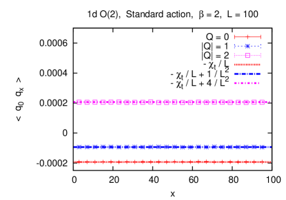
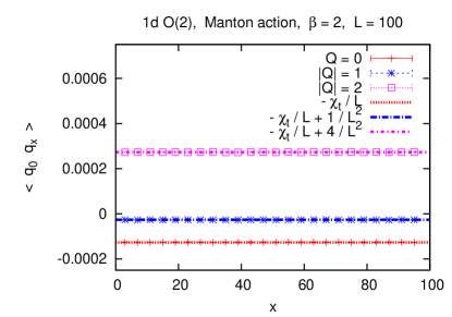
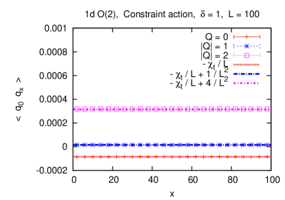
Figure 1: The topological charge density correlation in the 1d O(2) model over a distance of $x$ lattice spacings, at $L=100$. The first two plots refer to the standard action and the Manton action at $\beta=2$, with $\xi=2.779$, $\langle Q^{2}\rangle=1.936$, and $\xi=4.000$, $\langle Q^{2}\rangle=1.266$, respectively. The plot below is obtained with the constraint action at $\delta=1$, $L=100$, $\xi=5.793$, $\langle Q^{2}\rangle=0.844$. For comparison, we include in all cases horizontal lines for the prediction based on eq. (3.3), where we insert the directly measured values of $\chi_{\rm t}\,$.

In the thermodynamic limit, $L\to\infty$, the correlation length $\xi=1/(E_{1}-E_{0})$ (i.e. the inverse energy gap) and $\chi_{\rm t}$ are known analytically [10, 16], as we summarize in Table 1. The product $\xi\,\chi_{\rm t}$ is a scaling quantity, i.e. a dimensionless term composed of observables. In the continuum it amounts to

$$\xi\,\chi_{\rm t}|_{\rm continuum}=\frac{1}{2\pi^{2}}\ .$$ (3.7)

This value is attained for the lattice actions in the limit $\beta\to\infty$ and $\delta\to 0$, respectively, which reveals a facet of universality even in one dimension. The corresponding scaling behavior is discussed in Refs. [10, 18, 16]. In particular, the Manton action scales excellently, since it is classically perfect.

Figure 1 shows examples for numerically measured correlations $\langle q_{0}\,q_{x}\rangle_{|Q|}$, using these actions at $L=100$. We see in all cases that the numerical data are in excellent agreement with the predicted plateau values. These plateaux are accurately visible, so the AFHO method does indeed enable a precise numerical determination of $\chi_{\rm t}$.

To demonstrate this explicitly, we consider the range $L=150\dots 400$, and $|Q|=0,\ 1,\ 2$, which leads to the results for $\chi_{\rm t}$ in Figure 2. For the Manton action we obtain precise agreement with the theoretical $\chi_{\rm t}$ value in all cases. For the standard action we observe small deviations up to a few permille, which are suppressed for $|Q|\leq 1$, and for $|Q|=2$ they are reduced as $L$ increases.

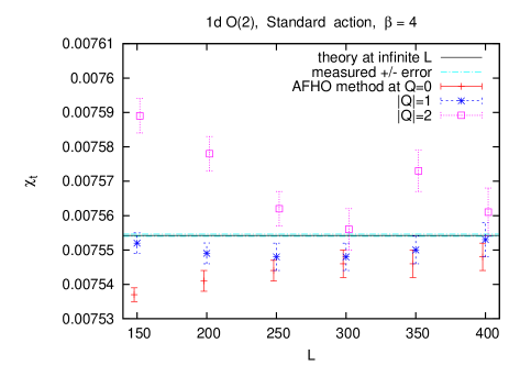
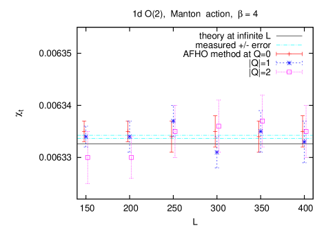
Figure 2: The topological susceptibility $\chi_{\rm t}$ in the 1d O(2) model for the standard and Manton action at $\beta=4$, where $\xi=6.8$ and $8.0$, respectively. We show the theoretical value at $L=\infty$, the directly measured value (at $L=400$), and the values obtained from the AFHO method in the range $L=150\dots 400$, in the sectors $|Q|=0,\ 1,\ 2$. For the standard action, there are permille level deviations from the predicted value, in particular for $|Q|=2$, which are suppressed for increasing $L$. For the Manton action all results coincide to an impressive precision, even down to $L=150$.

These tiny lattice artifacts are revealed due to extremely large statistics: for each parameter set, at least $5\cdot 10^{9}$ measurements have been performed with a cluster algorithm. This yields very precise results, and illustrates the convergence towards the theoretical $\chi_{\rm t}$ value for increasing $\langle Q^{2}\rangle$ (or equivalently $L$).

4 Results for the 2d O(3) model

We proceed to field theory, and first to the 2d O(3) model (or Heisenberg model), with periodic boundary conditions. In its lattice formulation a classical spin variable of unit length is attached to each lattice site $x$, $\vec{e}_{x}\in S^{2}$.

Regarding the topological charge, we consider sets of three neighboring spins. In our case the lattice consists of quadratic plaquettes, and each plaquette is divided into two triangles (the cutting diagonal has an alternating orientation between nearest neighbor plaquettes). Each of these triangles carries such a set of spins $\vec{e}_{1},\,\vec{e}_{2},\,\vec{e}_{3}$. They are connected on the sphere $S^{2}$ by the arcs of minimal length to form a spherical triangle. Its oriented area $A$ is given by [16]

$$x = 1+\vec{e}_{1}\cdot\vec{e}_{2}+\vec{e}_{2}\cdot\vec{e}_{3}+\vec{e}_{1}\cdot\vec{e}_{3}\ ,\quad y=\vec{e}_{1}\cdot(\vec{e}_{2}\times\vec{e}_{3})\ ,$$

$$\varphi = {\rm arg}(x+{\rm i}y)\ \mbox{mod}\ 2\pi\ ,\quad A(\vec{e}_{1},\vec{e}_{2},\vec{e}_{3})=2\varphi\ ,$$ (4.1)

where the modulo function is defined as in eq. (3.1). In each plaquette, the normalized sum of these two oriented spherical triangles (the total solid angle), $q_{x}=A(\vec{e}_{x},\vec{e}_{x+\hat{1}},\vec{e}_{x+\hat{2}},\vec{e}_{x+\hat{1}+\hat{2}})/(4\pi)$, is the topological charge density.

If we sum over all plaquettes, and thus over all triangles, we obtain the geometrically defined topological charge

$$Q=\sum_{x}q_{x}=\frac{1}{4\pi}\sum_{x}A(\vec{e}_{x},\vec{e}_{x+\hat{1}},\vec{e}_{x+\hat{2}},\vec{e}_{x+\hat{1}+\hat{2}})\in\mathbb{Z}\ .$$ (4.2)

This definition, which was advocated in Ref. [19], has the virtue of providing integer $Q$ values for all configurations (except for a subset of measure zero), just like eq. (3.2). It counts how many times (and with which orientation) these triangles cover the sphere.

The standard lattice action reads

$$S_{\rm standard}[\vec{e}\,]=\beta\sum_{x,\mu}(1-\vec{e}_{x}\cdot\vec{e}_{x+\hat{\mu}})\ ,$$ (4.3)

where $\mu$ runs from 1 to 2, $\hat{\mu}$ is the unit vector in $\mu$-direction, and $\beta>0$.

Figure 3 shows the topological charge density correlation $\langle q_{0}\,q_{x}\rangle$ at $\beta=1$, measured in the sectors $|Q|=0,\ 1,\ 2$, on $L\times L$ lattices of size $L=12$ and $L=16$. The measurements are carried out parallel to the axes, and the spin separation proceeds in steps of two lattice units, due to the alternating triangularization in the definition of $q_{x}$. The horizontal lines are the expected plateau values according to eq. (3.3). Again we inserted the directly measured values of $\chi_{\rm t}=\langle Q^{2}\rangle/V$; they are very precise, thanks to the use of a cluster algorithm, which provided a statistics of $O(10^{7})$ well thermalized and decorrelated measurements.

The plots clearly confirm the qualitatively expected picture. We further confirm that the condition of a large separation is quite harmless: for the separation of four lattice spacings, the plateau value is already well attained.

For a quantitative analysis, we perform individual fits of the data to a constant in one sector (skipping $2\dots 6$ points at the boundaries); each fit yields a value of the topological susceptibility $\chi_{\rm t}$. In addition we consider combined fits in two or three sectors. These results are confronted with the directly measured values in Figure 4. As theory predicts, the lowest $|Q|$-sectors are most reliable. In fact, the evaluation of $\chi_{\rm t}$ based on $\langle q_{0}\,q_{x}\rangle_{|Q|}$ is successful to an accuracy of a few percent in these cases. However, Figure 3 also shows that the application of this method is getting difficult when $L$ increases: then the values of $\langle q_{0}\,q_{x}\rangle_{|Q|}$ become tiny, and thus hard to distinguish from zero, and from each other.

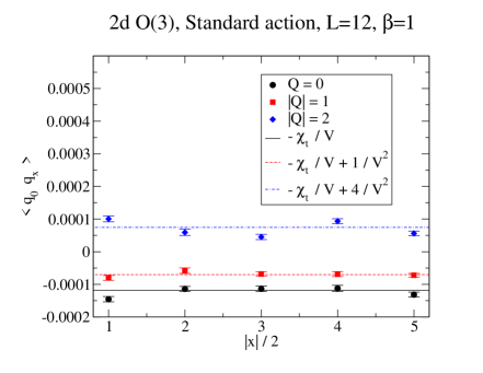
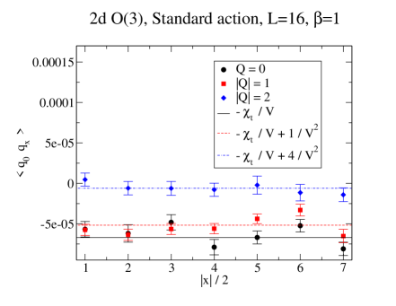
Figure 3: The topological charge density correlation in the 2d O(3) model, with the standard lattice action at $\beta=1$. We show data measured on $L\times L$ lattices, $L=12$ and $16$, in the sectors $|Q|=0,\,1,\,2$. They are compared to lines for the values according to eq. (3.3), with the directly measure susceptibility $\chi_{\rm t}$.

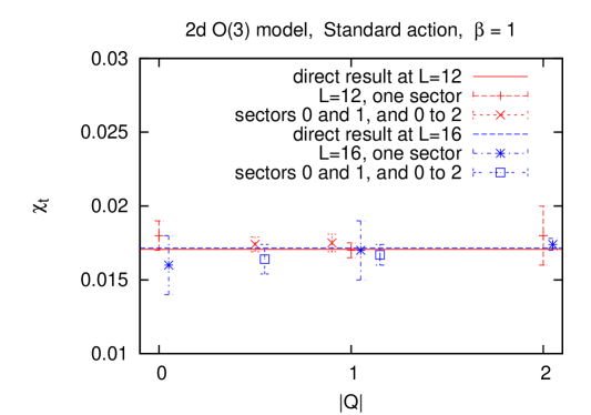
Figure 4: The topological susceptibility in the 2d O(3) model on $12\times 12$ and $16\times 16$ lattices, with the standard action at $\beta=1$. We show results obtained from fits to the topological charge density correlation in sector $|Q|$, or combined fits in several sectors. This is compared to the direct measurement as $\langle Q^{2}\rangle/V$, which is very precise. All results are compatible within the errors.

This is a case of strong coupling; $\beta=1$ leads to a correlation length of $\xi\simeq 1.3$ (at large $L$). Hence the volumes that we used can be considered large, but the lattice is coarse. In order to probe the AFHO method closer to the continuum limit, we now proceed to a different setting. We move to the constraint action, which is defined in analogy to eq. (3.6), i.e. the action is zero if all angles between neighboring spins are less than $\delta$, and infinite otherwise [16]. We set the constraint angle to $\delta=0.55\,\pi$, which corresponds to a correlation length of $\xi\simeq 3.6$. Accordingly, we now consider larger square lattices, with $L=16$ and $L=32$. Figure 5 shows the topological charge correlations in this case, and Figure 6 displays the fit results.

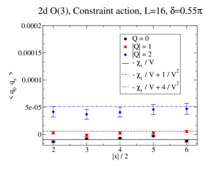
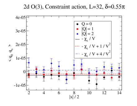
Figure 5: Plots analogous to Figure 3, now for the constraint action at $\delta=0.55\,\pi$, which corresponds to $\xi\simeq 3.6$, and with lattice sizes $L=16$ and $L=32$.

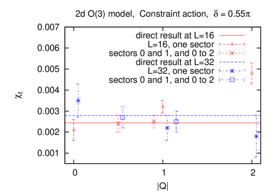
Figure 6: The topological susceptibility in the 2d O(3) model on $16\times 16$ and $32\times 32$ lattices, with the constraint action at $\delta=0.55\,\pi$, where $\xi\simeq 3.6$. We display results from fits to the topological charge density correlation in sector $|Q|$, or combined fits in several sectors. Comparison to the direct measurement shows that the AFHO method is less successful than in the examples of Figure 4, since larger volumes are involved.

These plots show again that the condition of a larger separation $|x|$ is not a practical problem. However, despite the statistics of $O(10^{7})$ measurements, the AFHO method does run into trouble in reproducing the directly measured $\chi_{\rm t}$ values beyond one digit. This is mostly a consequence of the larger volumes involved; they suppress the signal, which is relevant to extract $\chi_{\rm t}$ in this indirect manner.

Let us finally take a large step to a numerical experiment very close to the continuum limit: it is performed with the standard lattice action at $\beta=1.5$, on square lattices with $L=16\dots 128$; at large $L$, this corresponds to $\xi\simeq 9.5$. Figure 7 shows the results for $\chi_{\rm t}$ up to $L=84$, based on the topological charge correlations in the sectors $|Q|=0,\,1,\,2$, and by direct measurement. As $L$ increases, the latter converges well at $L\geq 32$. The results by the AFHO method move towards the directly measured value, and get close to it at $L=40$. Here the range $L\approx 40\dots 60$ is optimal for its application. As we increase $L$ further, we face again the problem that the tiny signal, which matters for $\chi_{\rm t}$, gets lost in the statistical noise. For $|Q|=1,\,2$ this happens already at $L\geq 64$; only at $Q=0$ the method still leads to useful results up to $L=84$. (For completeness we add that at $L=128$ we obtained $\chi_{\rm t}=0.0019(8)$, which is still compatible with the directly measured value $0.002292(9)$, but it has an error of $42~{}\%$).

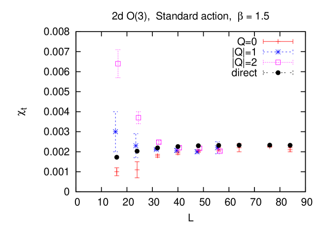
Figure 7: The topological susceptibility $\chi_{\rm t}$ for the standard action at $\beta=1.5$, on $L\times L$ lattices with $L=16\dots 84$ (with $\xi\simeq 9.5$ at large $L$). The directly measured values stabilize for $L\geq 32$ (its errors are too small to be visible in this plot), and the AFHO results approximate it well in the regime $L=40\dots 84$. For smaller $L$, this method suffers from significant finite size effects, and for larger $L$ the signal for the determination of $\chi_{\rm t}$ is too small for a good numerical resolution.

5 Results for 2d Abelian gauge theory

We proceed to 2d U(1) gauge theory with the plaquette action, i.e. Wilson’s standard lattice formulation [20]. We simulate it with the heatbath algorithm on periodic $L\times L$ lattices, with a variety of $L$ and $\beta$ values, which keep $\langle Q^{2}\rangle$ in the range of $0.7$ to $10.4$. In each case, the statistics involves $10^{7}$ configurations. For the topological charge density $q_{x}$ we also applied the straight plaquette regularization of the field strength tensor in terms of non-compact link variables $A_{x,\mu}$,

$$q_{x}=F_{x,12}=\frac{1}{2\pi}\Big{[}(A_{x,1}+A_{x+\hat{1},2}-A_{x+\hat{2},1}-A_{x,2})\ {\rm mod}\ 2\pi\Big{]}\ ,$$ (5.1)

still with the modulo function as defined in eq. (3.1). As in Section 4, its correlation was measured parallel to one of the axes.

Thanks to a generous separation of the measurements, the direct evaluation of $\chi_{\rm t}$ is very precise, although the updates are local.

Figure 8 gives three examples which illustrate that also here the data for the topological charge density match the predicted plateaux well, so that the determination of $\chi_{\rm t}$ by the AFHO method is possible. In addition we see again the difficulty setting in as the volume increases.

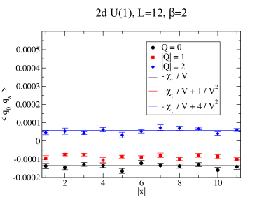
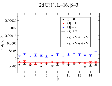
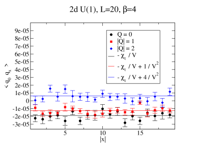
Figure 8: The topological charge density correlation in 2d U(1) gauge theory on $L\times L$ lattices, over a distance of $x$ lattice spacings. We show the first three plateau values (horizontal lines, based on direct measurements of $\chi_{\rm t}$), and the corresponding data for $\beta=2$, $L=12$, with a plaquette value of $\langle P\rangle=0.6978$ and $\langle Q^{2}\rangle=2.79$; $\beta=3$, $L=16$, $\langle P\rangle=0.8100$, $\langle Q^{2}\rangle=2.83$, and $\beta=4$, $L=20$, $\langle P\rangle=0.8635$, $\langle Q^{2}\rangle=3.02$.

Figure 9 provides an overview over the results in the range $L=6\dots 20$ and $\beta=1\dots 5$. In the extreme cases, the plaquette values amount to $\langle P\rangle=0.4464$ ($\beta=1$) and $0.8934$ ($\beta=5$); for the rest we refer to the caption of Figure 8.

In this case, we apply the AFHO method as a combined fit to the data in the topological sectors with $Q=0$ and $|Q|=1$. This might be the optimal application, which includes a large number of data points, but avoids the less reliable topological sectors. In all the cases shown in Figure 9, these AFHO results for $\chi_{\rm t}$ agree with the directly measured values, within errors on the percent level, e.g. at $L=16$ we obtain $\chi_{\rm t}=0.0196(6)\ (\beta=2)$;  $0.0110(3)\ (\beta=3)$;  $0.0075(2)\ (\beta=4)$.

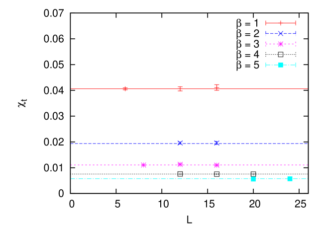
Figure 9: The topological susceptibility $\chi_{\rm t}$ for 2d U(1) gauge theory, on $L\times L$ lattices. The horizontal lines are the directly measured values (errors and differences for various $L$ are invisible on this scale). The symbols are the AFHO values obtained by a combined fit in the sectors $|Q|\leq 1$.

In contrast to the previous sections, we are now dealing with a local update algorithm, which is the situation that motivates this project. As an illustrative example, we add a measurement of the integrated autocorrelation time $\tau_{\rm int}$ (for the definition, see e.g. Ref. [21]) with respect to $Q$. It is expressed in the number of sweeps (updates of each link variable), in a fixed volume with $L=16$. Figure 10 shows that $\tau_{\rm int}$ increases rapidly as we approach the continuum limit. This confirms that, for the heatbath algorithm, the problem of “topological freezing” becomes severe indeed, once we attain plaquette values of $\langle P\rangle\gtrsim 0.9$. (The results in Figures 8 and 9 were obtained by separating the measurements by a number of sweeps, which clearly exceeds $\tau_{\rm int}$).

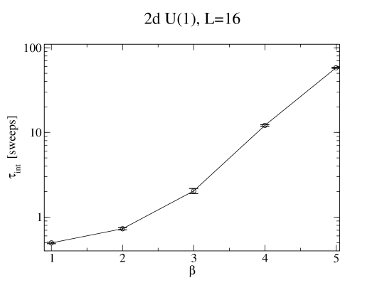
Figure 10: The integrated autocorrelation time $\tau_{\rm int}$ in 2d U(1) gauge theory, with respect to the topological charge $Q$. We consider $\beta=1\dots 5$ on a $16\times 16$ lattice, and measure $\tau_{\rm int}$ based on $10^{7}$ sweeps, after thermalization. As $\beta$ is getting large, we observe an exponential increase of $\tau_{\rm int}$ (measured in the number of sweeps).

6 Results for 4d SU(2) Yang-Mills theory

Finally we study 4d SU(2) Yang-Mills theory, which is in many respects close to QCD, but computationally cheaper. Therefore, tests in SU(2) Yang-Mills theory are ideal for hints about the practical applicability of the AFHO method to QCD. As usual, the lattice gauge field is represented in terms of compact link variables $U_{x,\mu}\in{\rm SU(2)}$ [20].

Following Ref. [22], we determine the topological charge density $q_{x}$, and the topological charge $Q=\sum_{x}q_{x}$, by an improved field theoretic definition,

$$q_{x}[U]=\frac{1}{16\pi^{2}}\sum_{\mu\nu\rho\sigma}\epsilon_{\mu\nu\rho\sigma}\sum_{\Box=1,2,3}\frac{c_{\Box}}{\Box^{4}}F_{x,\,\mu\nu}^{(\Box\times\Box)}[U]\ F_{x,\,\rho\sigma}^{(\Box\times\Box)}[U]\ ,$$ (6.1)

where $F_{x,\,\mu\nu}^{(\Box\times\Box)}$ denotes the dimensionless lattice field strength tensor, clover averaged over square-shaped Wilson loops of size $\Box\times\Box$, and $c_{1}=1.5$, $c_{2}=-0.6$, $c_{3}=0.1$.

We apply eq. (6.1), after performing a number $N_{\rm cool}$ of cooling sweeps with the intention to suppress UV fluctuations in the gauge configurations, while preserving the topological structure. A cooling sweep amounts to a local minimization of the action, i.e. a successive minimization with respect to each gauge link. For this minimization we also use an improved version of the lattice Yang-Mills action,

$$S[U]=\frac{\beta}{16}\sum_{x}\sum_{\mu\nu}\sum_{\Box=1,2,3}\frac{c_{\Box}}{\Box^{4}}\textrm{Tr}\Big{(}1-W_{x,\,\mu\nu}^{(\Box\times\Box)}[U]\Big{)}\ ,$$ (6.2)

where $\beta=1/(4g^{2})$, and $W_{x,\,\mu\nu}^{(\Box\times\Box)}$ is a clover averaged loop of size $\Box\times\Box$. Choosing an appropriate sweep number $N_{\textrm{cool}}$ is a subtle and somewhat ambiguous task, which will be discussed below.

The lattice action used for the generation of gauge configurations is the standard plaquette action, which is obtained from eq. (6.2) by setting $c_{1}=1$, $c_{2}=c_{3}=0$. As in Section 5, the simulations were performed with a heatbath algorithm [20], now at $\beta=2.5$. This corresponds to the lattice spacing $a\approx 0.073\,\textrm{fm}$, when the scale is set by identifying the Sommer parameter $r_{0}$ with $0.46\,\textrm{fm}$ [23]. That value of $a$ is in the range of lattice spacings $0.05\,\textrm{fm}\leq a\leq 0.15\,\textrm{fm}$ typically used in contemporary QCD simulations. We generated about 4000 configurations in each of three volumes, $V=14^{4}\,,\ 16^{4}\,,\ 18^{4}$. This is also a typical statistics in QCD simulations.

Assigning a topological charge $Q$ to each configuration leads to the statistics given in Table 2 for the sectors $|Q|\leq 4$. We proceed by computing the correlation function of the topological charge density $\langle q_{0}q_{x}\rangle_{|Q|}$ in all these sectors $Q$ and volumes $V$.

The normalization factor on the right-hand-side of eq. (2.1) is given by the inverse volume. As we have observed in the previous sections, the correspondingly suppressed signal in a large volume is often the bottleneck in the application of the AFHO method. In order to compensate this suppression, which is worrisome in a 4d volume, we now determine $\langle q_{0}q_{x}\rangle$ by measuring all-to-all correlations in each configuration, thus taking advantage of the discrete translational and rotational invariance.

In a second step we fit to these lattice results the right-hand-side of eq. (3.3), i.e. eq. (2.1) with $c_{4}=0$, with respect to $\chi_{\rm t}$, at sufficiently large separations $x$, where $\langle q_{0}q_{x}\rangle_{|Q|}$ exhibits a plateau.

$V$	$Q=0$	$|Q|=1$	$|Q|=2$	$|Q|=3$	$|Q|=4$
$14^{4}$	1023	1591	0893	0350	0103
$16^{4}$	0722	1371	0942	0574	0248
$18^{4}$	0622	1079	0898	0616	0402

Table 2: Number of configurations for three volumes $V$, in each topological sector $0\leq|Q|\leq 4$. The topological charge has been assigned after performing $N_{\textrm{cool}}=10$ cooling sweeps.

Figure 11 illustrates the determination of $\chi_{\rm t}$ after $N_{\textrm{cool}}=10$ cooling sweeps, in the three lattice volumes under consideration. Clearly the correlation function $\langle q_{0}q_{x}\rangle_{|Q|}$ is different for each topological sector $|Q|$. These differences are more pronounced for smaller volumes $V$ and larger topological charges $Q$, which shows that the splitting according to eqs. (2.1) and (3.3) can indeed be resolved from our data. Hence the statistics, drastically amplified by the all-to-all correlations, is indeed sufficient to reveal the relevant signal.

In particular, for $V=14^{4}$ the maximally available on-axis separations $|x|=6,7,8$ are at the border-line which allows us to observe plateaux of $\langle q_{0}q_{x}\rangle_{|Q|}$. For $V=16^{4}$ plateaux are visible in the range $|x|=7,8,9$ and in $V=18^{4}$ even five points, $7\leq|x|\leq 11$, are consistent with a plateau.

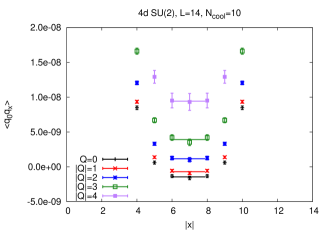
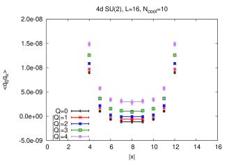
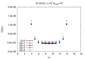
Figure 11: The correlation $\langle q_{0}q_{x}\rangle_{|Q|}$ as a function of the on-axis separation $|x|$, after $N_{\textrm{cool}}=10$ cooling sweeps, for the lattice volumes $V=14^{4}\,,\ 16^{4}\,,\ 18^{4}$. Fits of the right-hand-side of eq. (3.3) with respect to $\chi_{\rm t}$ are indicated by the horizontal solid lines.

Since the signal, i.e. the differences between the plateau values, increases for smaller volumes, a promising strategy might be to use anisotropic volumes. For example the volumes of a $14^{4}$ and a $12^{3}\times 24$ lattice are similar (i.e. both should exhibit a similar signal quality), but the latter allows to study larger separations (on-axis up to $|x|=12$, though not with the entire statistics of all-to-all correlations).

In Figure 12 we show determinations of $\chi_{\rm t}$ and compare different numbers of cooling sweeps, $N_{\textrm{cool}}=5\,,\ 10\,,\ 20$, in the volumes $V=14^{4}$ and $18^{4}$. For a small number, such as $N_{\textrm{cool}}=5$, the correlation function $\langle q_{0}q_{x}\rangle_{|Q|}$ is rather noisy. This is a consequence of strong UV fluctuations, which are manifest in the topological charge density $q_{x}$, and which are not filtered out sufficiently at small $N_{\textrm{cool}}$. For a large number of cooling sweeps, like $N_{\textrm{cool}}=20$, statistical errors are significantly smaller, but the correlation function $\langle q_{0}q_{x}\rangle_{|Q|}$ exhibits plateaux only at larger separations $|x|$.

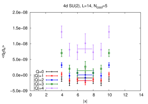
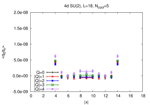
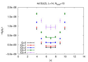
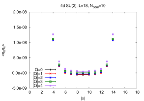
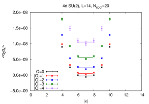
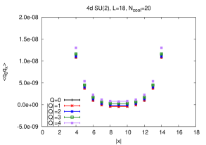
Figure 12: The correlation $\langle q_{0}q_{x}\rangle_{|Q|}$ as a function of the on-axis separation $|x|$ for different numbers of cooling sweeps, $N_{\textrm{cool}}=5\,,\ 10\,,\ 20$, and lattice volumes $V=14^{4}$ and $18^{4}$.

This effect becomes plausible when considering the structure of the states contributing to $\langle q_{0}q_{x}\rangle_{|Q|}$. This correlation function is the Fourier transform of an analogous correlation function, summed over all topological sectors at a finite vacuum angle $\theta$ (for a detailed discussion, see Ref. [17]). The plateau values arise due to the non-vanishing vacuum expectation value $\langle q_{x}\rangle$ at $\theta\neq 0$. Deviations from these plateaux are predominantly caused by low-lying excitations, which correspond to glueballs in Yang-Mills theory. Due to the glueball size, the overlap with $q_{x}|\Omega\rangle$ (where $|\Omega\rangle$ is the vacuum state) increases when using extensive cooling (then $q_{x}$ is an extended operator resembling a low-lying glueball), compared to little or no cooling (then $q_{x}$ is a highly local operator). Consequently, cooling enhances the contribution of excitations to the correlation function $\langle q_{0}q_{x}\rangle_{|Q|}$ and, hence, causes stronger deviations from the plateaux.

In practice one should decide for an optimal compromise, i.e. an intermediate number of cooling sweeps. Such a compromise can be read off for instance from plots showing the dependence of the topological susceptibility $\chi_{\rm t}$ (obtained by the AFHO method at fixed $|Q|$), or the correlation function $\langle q_{0}q_{x}\rangle_{|Q}$ at specific separation $|x|\approx L/2$ on $N_{\textrm{cool}}$. Such plots are shown in Figure 13 for $L=18$ and fixed topological charge $|Q|=0,1,2$. As expected, the statistical errors are quite large for small $N_{\textrm{cool}}\raisebox{-2.15277pt}{$\,\stackrel{{\scriptstyle<}}{{\scriptstyle\sim}}\,$}5$. In an intermediate region, $5\raisebox{-2.15277pt}{$\,\stackrel{{\scriptstyle<}}{{\scriptstyle\sim}}\,$}N_{\textrm{cool}}\raisebox{-2.15277pt}{$\,\stackrel{{\scriptstyle<}}{{\scriptstyle\sim}}\,$}15$, there are stable plateaux of both $\langle q_{0}q_{x}\rangle_{|Q|}$ and $\chi_{\rm t}$ with comparably small statistical errors. The rather long plateaux indicate that cooling is a numerically stable procedure, not destroying topological excitations nor introducing any unwanted non-locality effects. At large $N_{\textrm{cool}}\raisebox{-2.15277pt}{$\,\stackrel{{\scriptstyle>}}{{\scriptstyle\sim}}\,$}15$ there is a slight trend towards lower $\chi_{\rm t}$, in particular for $Q=0$, which could be a first sign of contamination by excited states. An optimal choice for $N_{\textrm{cool}}$ is somewhere inside the plateaux region, such as $N_{\textrm{cool}}=8$ or $N_{\textrm{cool}}$ = 10, as we have used in the examples in Figure 11 and Table 3.

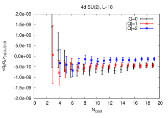
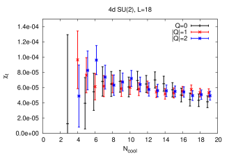
Figure 13: The correlation $\langle q_{0}q_{x}\rangle_{|Q|}$ at $|x|=L/2=9$, and the topological susceptibility $\chi_{\rm t}$, as a function of the number of cooling sweeps $N_{\textrm{cool}}$ in the volume $V=18^{4}$.

Numerical results for the larger volumes, $V=16^{4}$ and $18^{4}$, and moderate cooling, $N_{\textrm{cool}}=8$ or $10$, where a reasonably accurate determination of $\chi_{\rm t}$ seems possible, are summarized in Table 3. Fits have been restricted to sectors $Q$ fulfilling $|Q|/(\chi_{\rm t}V)<0.5$, which involves the small expansion parameter in the derivation of eq. (2.1) [5, 17]. The resulting values for the topological susceptibility agree within the errors with a previous straight determination (without topology fixing), which arrived at $\chi_{\rm t}=7.0(9)\times 10^{-5}$ [22].

$V$	$N_{\textrm{cool}}$	$Q=0$	$|Q|=1$	$|Q|=2$	$|Q|=3$	combined
$16^{4}$	08	$6.1(9)$	$5.5(9)$	$7.1(8)$		$6.3(6)$
	10	$7.4(10)$	$5.4(7)$	$6.5(9)$		$6.3(5)$
$18^{4}$	08	$7.1(14)$	$~{}\,5.8(10)$	$~{}\,7.4(12)$	$9.2(19)$	$7.3(6)$
	10	$6.2(10)$	$~{}\,5.9(10)$	$6.6(9)$	$8.7(11)$	$7.0(5)$

Table 3: Results for the topological susceptibility $\chi_{\rm t}\times 10^{5}$ extracted from fits to a single sector $|Q|$, or combined fits to several sectors ($0\leq|Q|\leq 2$ for $V=16^{4}$, $0\leq|Q|\leq 3$ for $V=18^{4}$). A corresponding study without topology fixing [22] obtained $\chi_{\rm t}\times 10^{5}=7.0(9)$.

We also investigated the magnitude of ordinary finite volume effects, (not related to topology fixing). We did this by computing and comparing $\chi_{\rm t}$ at unfixed topology using $\chi_{\rm t}=\langle Q^{2}\rangle/V$. For the three volumes used throughout this section, and $N_{\textrm{cool}}=10$, we obtain for $\chi_{\rm t}(V)$

$$\chi_{\rm t}(14^{4})=7.02(1)\times 10^{-5},\ \chi_{\rm t}(16^{4})=6.97(2)\times 10^{-5},\ \chi_{\rm t}(18^{4})=7.01(3)\times 10^{-5}.$$

These values agree within the statistical errors. Moreover, both the differences as well as the statistical errors are significantly smaller (by more than a factor of $10$) than the uncertainties associated with our $\chi_{\rm t}$ determinations using the AFHO method, as listed in Table 3. Therefore, in our study ordinary finite volume effects can safely be neglected.

The similarity of 4d SU(2) Yang-Mills theory and QCD suggests that an application of the AFHO method to QCD will also allow for a determination of the topological susceptibility up to about $10\,\%$, based on $O(1000)$ configurations for each of the topological sectors with small $|Q|$. We plan to explore this scenario in the near future.

7 Conclusions

We have investigated the AFHO method [5] for the evaluation of the topological susceptibility $\chi_{\rm t}$ based on the correlation of the topological charge density. Amazingly, this method allows — in principle — for a measurement of $\chi_{\rm t}$ even within a fixed topological sector, and low $|Q|$ are most promising.

We have seen that the method as such works; in some cases it provided results, which are correct to 2 or 3 digits. Hence situations do exist, where the approximations in the derivation of formula (3.3) (in particular including order $O(1/V^{2})$ incompletely, and neglecting all terms of $O(1/V^{3})$) can be justified, as we could confirm on the non-perturbative level.

This approximation neglects the kurtosis term in relation (2.1), and all higher terms. They are suppressed by the inverse volume. Moreover, it is a generic property that topological charges are approximately Gauss distributed, such that $|c_{4}|$ is small. As a peculiar case, it vanishes in the continuum 1d O(2) model, and in that case there are no higher corrections either (cf. Appendix A).

Regarding the limitations of the applicability range, we note that — for most models studied here — the theoretical condition of measuring the correlation “at large separation” turned out not to be worrisome in practice; only in Section 6 this issue has some relevance. However, the AFHO method generally runs into trouble when the volume $V$ increases. Then the signal in $\langle q_{0}\,q_{x}\rangle_{|Q|}$ is suppressed by a factor $1/V$, and the separation between the predicted plateaux by $1/V^{2}$. If we want the correlation length to be clearly larger than the lattice spacing (so that lattice artifacts are under control), we need a sizable lattice to keep the finite size effects under control as well. With these conflicting requirements, even in our 2d test models, and despite a statistics of $10^{7}$ measurements, this method led to results with rather large statistical errors.

Thus we observe that the AFHO method, which is based on topologically restricted measurements, is plagued by unusually persistent finite size effects. In usual settings, the latter are exponentially suppressed, i.e. they are $\propto\exp(-{\rm const.}\,L/\xi)$, and quite small if $L/\xi\gtrsim 4$. However, topologically restricted numerical measurements are very sensitive to finite size effects: we recall that relation (2.1) is a truncated polynomial expansion in $1/V$, but we can also refer directly to the large ratios $L/\xi$, which were used all over this study: e.g. in the upper plot of Figure 2 it amounts to $L/\xi>22$, which usually makes finite size effects negligible, but here they are significant. This property calls for a larger size $L$. In turn, that causes problems in extracting the subtle effect, which is relevant for the indirect determination of $\chi_{\rm t}$.

That issue might be the bottleneck for the prospects to apply the AFHO method in four dimensions, and it has inspired the approach of restriction to sub-volumes [13]. However, our study in Section 6 shows that the suppression of the wanted signal by the inverse volume can be successfully compensated if we enhance the statistics by means of all-to-all correlation measurements. We have seen in 4d SU(2) Yang-Mills theory that this procedure does provide sufficient precision for $\langle q_{0}q_{x}\rangle$, even for a moderate number of $O(1000)$ configurations in one topological sector. Due to this observation, the AFHO method in its original form appears quite promising in QCD. We are going to test if it enables also there the evaluation of $\chi_{\rm t}$ in an unconventional way, to an accuracy of about $10\,\%$.

Acknowledgements  Lilian Prado has worked on this project at an early stage. We also thank Christopher Czaban and Philippe de Forcrand for interesting discussions. This work was supported in part by the Mexican Consejo Nacional de Ciencia y Tecnología (CONACYT) through project 155905/10, by DGAPA-UNAM, grant IN107915, and by the Helmholtz International Center for FAIR within the framework of the LOEWE program launched by the State of Hesse. A.D. and M.W. acknowledge support by the Emmy Noether Programme of the DFG (German Research Foundation), grant WA 3000/1-1, and C.P.H. acknowledges support through the project Redes Temáticas de Colaboración Académica 2013, UCOL-CA-56. Calculations on the LOEWE-CSC and on the FUCHS-CSC high-performance computer of the Frankfurt University were conducted for this project. We would like to thank HPC-Hessen, funded by the State Ministry of Higher Education, Research and the Arts, for programming advice.

Appendix A Topological charge density correlation in the continuum 1d O(2) model

The key quantity of this work is the correlation function of the topological charge density. In this appendix we compute it analytically for the 1d O(2) model, formulated in continuous Euclidean time $x$, with periodicity length $L$. For this purpose, it is useful to include a $\theta$-term in the action,

$$S[\varphi]=\frac{\beta_{\rm cont}}{2}\int_{0}^{L_{\rm cont}}dx\,\varphi^{\prime}(x)^{2}-{\rm i}\theta Q[\varphi]\ .$$ (A.1)

In the canonical formulation of quantum mechanics, the corresponding Hamilton operator, its energy eigenfunctions and eigenvalues read [10]

$$\hat{H}=\frac{1}{2\beta_{\rm cont}}\ \Big{(}\hat{p}-\frac{\theta}{2\pi}\Big{)}^{2}\ ,\ \langle\varphi|n\rangle=\frac{1}{\sqrt{2\pi}}\ e^{{\rm i}n\varphi}\ ,\ E_{n}=\frac{1}{2\beta_{\rm cont}}\Big{(}n-\frac{\theta}{2\pi}\Big{)}^{2}\ ,\$$ (A.2)

where $\hat{p}=-{\rm i}\frac{\partial}{\partial\varphi}$ and $n\in\mathbb{Z}$. The operator for the topological charge density is given by

$$\hat{q} = \frac{1}{2\pi}[\hat{H},\hat{\varphi}]=\frac{1}{2\pi\beta_{\rm cont}}\Big{(}-\frac{\partial}{\partial\varphi}+{\rm i}\frac{\theta}{2\pi}\Big{)}\ .$$ (A.3)

This operator is anti-Hermitian (due to the Euclidean time derivative of the Hermitian operator $\hat{\varphi}$), with the matrix elements

$$\langle m|\hat{q}|n\rangle=\frac{1}{(2\pi)^{2}\beta_{\rm cont}}\int_{-\pi}^{\pi}d\varphi\,e^{-{\rm i}m\varphi}\,\Big{(}-\frac{\partial}{\partial\varphi}+{\rm i}\frac{\theta}{2\pi}\Big{)}\,e^{{\rm i}n\varphi}=\frac{{\rm i}(\theta-2\pi n)}{(2\pi)^{2}\beta_{\rm cont}}\,\delta_{mn}\ .$$

Hence the expectation value

$$\langle q(x)\rangle=\frac{1}{Z(\theta)}\frac{{\rm i}}{(2\pi)^{2}\beta_{\rm cont}}\sum_{n\in\mathbb{Z}}(\theta-2\pi n)\,e^{-E_{n}L_{\rm cont}}\ ,\ {\rm with}\ Z(\theta)=\sum_{n\in\mathbb{Z}}\,e^{-E_{n}L_{\rm cont}}$$

is imaginary in general (of course it vanishes at $\theta=0$).

Therefore the corresponding correlation function is in general negative,

$$\langle q(0)q(x)\rangle = \frac{1}{Z(\theta)}\sum_{m,n\in\mathbb{Z}}\langle m|\hat{q}|n\rangle\,\langle n|\hat{q}|m\rangle\,e^{-E_{n}x-E_{m}\,(L_{\rm cont}-x)}$$ (A.4)

$$= -\frac{1}{Z(\theta)}\frac{1}{(2\pi)^{4}\beta^{2}_{\rm cont}}\,\sum_{n\in\mathbb{Z}}(\theta-2\pi n)^{2}\,e^{-E_{n}L_{\rm cont}}\ .$$

It is remarkable that this correlation is independent of $x$, if $x/L_{\rm cont}\notin\mathbb{Z}$ (this condition allows us to insert a unit factor $\sum_{n}|n\rangle\langle n|$ between the end-points).

The vacuum angle $\theta$ enables also the computation of the topologically restricted partition function,

$$Z_{Q}=\frac{1}{2\pi}\int_{-\pi}^{\pi}d\theta\,Z(\theta)\,e^{-{\rm i}Q\theta}=\frac{1}{2\sqrt{\pi\alpha}}e^{-Q^{2}/(4\alpha)}\ ,\ \ \alpha=\frac{L}{8\pi^{2}\beta_{\rm cont}}\ ,$$

and correlation function,

$$\langle q(0)q(x)\rangle_{Q} = \frac{1}{2\pi Z_{Q}}\int_{-\pi}^{\pi}d\theta\,Z(\theta)\langle q(0)q(x)\rangle\,e^{-{\rm i}Q\theta}$$ (A.5)

$$= -\frac{1}{(2\pi)^{5}\beta^{2}_{\rm cont}Z_{Q}}\int_{-\infty}^{\infty}d\theta\,\theta^{2}\,e^{-\alpha\theta^{2}-{\rm i}\theta Q}$$

$$= \frac{1}{32\pi^{4}\beta^{2}_{\rm cont}\alpha}\Big{(}-1+\frac{Q^{2}}{2\alpha}\Big{)}\ .$$

Finally we insert $\alpha$ and $\chi_{\rm t}=\alpha L_{\rm cont}/2$ (cf. Table 1) to arrive at

$$\langle q(0)q(x)\rangle_{Q}=-\frac{\chi_{\rm t}}{L_{\rm cont}}+\frac{Q^{2}}{L^{2}_{\rm cont}}\ .$$ (A.6)

Also the topologically restricted correlation function is constant in $x$, which explains that the data in Section 3 attain the plateau values immediately.

Moreover, we see that eq. (3.3) is exact in this specific case, which is consistent with the fact that the kurtosis vanishes [10]. Therefore, in our numerical study presented in Section 3, the actual issues are lattice artifacts and the visibility of the predicted plateau values in numerical simulation data; both are generally relevant questions.

References

-
[1]
E. Witten, Nucl. Phys. B 156 (1979) 269.
G. Veneziano, Nucl. Phys. B 159 (1979) 213. -
[2]
K. Cichy, A. Dromard, E. Garcia-Ramos, K. Ottnad,
C. Urbach, M. Wagner, U. Wenger and F. Zimmermann,
arXiv:1411.1205 [hep-lat].
Y. Namekawa, arXiv:1501.06295 [hep-lat]. - [3] U. Wolff, Phys. Rev. Lett. 62 (1989) 361.
- [4] M. Lüscher, JHEP 1008 (2010) 071 [arXiv:1006.4518 [hep-lat]].
- [5] S. Aoki, H. Fukaya, S. Hashimoto and T. Onogi, Phys. Rev. D 76 (2007) 054508 [arXiv:0707.0396 [hep-lat]].
- [6] Ph. de Forcrand, M. García Pérez, J.E. Hetrick, E. Laermann, J.F. Lagae and I.O. Stamatescu, Nucl. Phys. (Proc. Suppl.) 73 (1999) 578 [hep-lat/9810033].
- [7] R.C. Brower et al. (LSD Collaboration), Phys. Rev. D 90 (2014) 014503 [arXiv:1403.2761 [hep-lat]].
- [8] R. Brower, S. Chandrasekharan, J.W. Negele and U.-J. Wiese, Phys. Lett. B 560 (2003) 64 [hep-lat/0302005].
-
[9]
L. Del Debbio, L. Giusti and C. Pica,
Phys. Rev. Lett. 94 (2005) 032003
[hep-th/0407052].
W. Bietenholz and S. Shcheredin, Nucl. Phys. B 754 (2006) 17 [hep-lat/0605013].
S. Dürr, Z. Fodor, C. Hoelbling and T. Kurth, JHEP 0704 (2007) 055 [hep-lat/0612021].
M. Cé, C. Consonni, G.P. Engel and L. Giusti, arXiv:1506.06052 [hep-lat]. - [10] W. Bietenholz, R. Brower, S. Chandrasekharan and U.-J. Wiese, Phys. Lett. B 407 (1997) 283 [hep-lat/9704015].
- [11] W. Bietenholz, I. Hip, S. Shcheredin and J. Volkholz, Eur. Phys. J. C 72 (2012) 1938 [arXiv:1109.2649 [hep-lat]].
- [12] S. Aoki et al. (JLQCD and TWQCD Collaborations), Phys. Lett. B 665 (2008) 294 [arXiv:0710.1130 [hep-lat]].
- [13] H. Fukaya, S. Aoki, G. Cossu, S. Hashimoto, T. Kaneko and J. Noaki (JLQCD Collaboration), PoS LATTICE2014 (2014) 323 [arXiv:1411.1473 [hep-lat]].
-
[14]
I. Bautista, W. Bietenholz, U. Gerber,
C.P. Hofmann, H. Mejía-Díaz and L. Prado,
arXiv:1402.2668 [hep-lat].
U. Gerber, I. Bautista, W. Bietenholz, H. Mejía-Díaz and C.P. Hofmann, PoS LATTICE2014 (2014) 320 [arXiv:1410.0426 [hep-lat]].
A. Dromard, W. Bietenholz, U. Gerber, Mejía-Díaz and Marc Wagner, arXiv:1510.08809 [hep-lat]. - [15] N. Manton, Phys. Lett. B 96 (1980) 328.
- [16] W. Bietenholz, U. Gerber, M. Pepe and U.-J. Wiese, JHEP 1012 (2010) 020 [arXiv:1009.2146 [hep-lat]].
- [17] A. Dromard and M. Wagner, Phys. Rev. D 90 (2014) 074505 [arXiv:1404.0247 [hep-lat]].
- [18] T. Boyer, W. Bietenholz and J. Wuilloud, Int. J. Mod. Phys. C 18 (2007) 1497 [cond-mat/0701331].
- [19] B. Berg and M. Lüscher, Nucl. Phys. B 190 (1981) 412.
-
[20]
M. Creutz, “Quarks, gluons and lattices,”,
Cambridge University Press, 1983.
I. Montvay and G. Münster, “Quantum Fields on a Lattice”, Cambridge University Press, 1994. - [21] F. Niedermayer, Lect. Notes Phys. 501 (1998) 36 [hep-lat/9704009].
- [22] P. de Forcrand, M. Garcia Perez and I.-O. Stamatescu, Nucl. Phys. B 499 (1997) 409 [hep-lat/9701012].
- [23] O. Philipsen and M. Wagner, Phys. Rev. D 89 (2014) 014509 [arXiv:1305.5957 [hep-lat]].
-
[24]
E. Seiler and I.O. Stamatescu,
preprint MPI-PAE/PTh 10/87.
E. Vicari, Nucl. Phys. B 554 (1999) 301 [hep-lat/9901008].
E. Seiler, Phys. Lett. B 525 (2002) 355 [hep-th/0111125].