THE ENVIRONMENT OF THE STRONGEST GALACTIC METHANOL MASER

Abstract

The high-mass star-forming site G009.62+00.20 E hosts the 6.7 GHz methanol maser source with the greatest flux density in the Galaxy which has been flaring periodically over the last ten years. We performed high-resolution astrometric measurements of the CH₃OH, H₂O, and OH maser emission and 7 mm continuum in the region. The radio continuum emission was resolved in two sources separated by 1300 AU. The CH₃OH maser cloudlets are distributed along two north-south ridges of emission to the east and west of the strongest radio continuum component. This component likely pinpoints a massive young stellar object which heats up its dusty envelope, providing a constant IR pumping for the Class II CH₃OH maser transitions. We suggest that the periodic maser activity may be accounted for by an independent, pulsating, IR radiation field provided by a bloated protostar in the vicinity of the brightest masers. We also report about the discovery of an elliptical distribution of CH₃OH maser emission in the region of periodic variability.

1 INTRODUCTION

G009.62+00.20 is a star-forming complex located at a parallax distance of 5.2 kpc from the Sun (Sanna et al., 2009, 2014). Its radio continuum source “E”, named by Garay et al. (1993), is the most compact component among a number of H ii regions detected in the field, which align along a ridge of 0.5 pc in size (e.g., Liu et al. 2011). Close to G009.62+00.20 E, the presence of an embedded, massive, young stellar object (YSO), is inferred through interferometric observations of high-excitation CH₃CN and CH₃OH lines, typical hot molecular core tracers, and continuum dust emission at 2.7 mm (Hofner et al., 1996, 2001). Source E has not been detected at near-infrared (Persi et al., 2003) or mid-infrared (Linz et al., 2005) wavelengths, which argues for an early stage of stellar evolution. Its continuum emission at 1.3 cm is unresolved with a beam size of about $0\farcs 3$ (Testi et al., 2000; Sanna et al., 2009), which sets an upper limit to the physical extent of the H ii emission of $\lesssim 0.01$ pc.

In proximity of source E, it is observed several Class II CH₃OH maser transitions (e.g., Phillips et al. 1998; Minier et al. 2002), including the strongest maser emission at 6.7 GHz observed in the Galaxy (5000-6000 Jy, Menten 1991), together with H₂O (Hofner & Churchwell, 1996), ground state OH (Fish et al., 2005), and a rare maser action in the NH₃ (5,5) inversion line (Hofner et al., 1994). An interesting characteristic of this object is the periodic variability of its Class II CH₃OH masers (van der Walt et al., 2009), with a cycle of 244 days over the 10 years monitoring performed so far (Goedhart et al., 2014).

In order to explain this intriguing behavior, it is crucial to image both the maser distribution and the H ii region morphology with high accuracy. For this purpose, we have performed astrometric observations toward G009.62+00.20 of the 6.7 GHz CH₃OH, 1.665 and 1.667 GHz OH, and 22.2 GHz H₂O masers with the Australian Long Baseline Array (LBA) and the Very Long Baseline Array (VLBA). Very Long Baseline Interferometry (VLBI) observations were performed in phase-referencing mode for the primary goal of absolute position calibration at milliarcsecond accuracy. We also conducted Karl G. Jansky Very Large Array (JVLA) observations in the most extended configuration at Q band, in order to accurately locate the H ii region with respect to the maser species and determine its brightness distribution.

2 OBSERVATIONS

2.1 MASERS

We employed the VLBA to observe the $6_{16}-5_{23}$ H₂O maser transition (at 22.235079 GHz) and both main-line ${}^{2}\Pi_{3/2}$ $\rm J=3/2$ OH maser transitions (at 1.665401 GHz and 1.667359 GHz). The LBA was used to observe the $5_{1}-6_{0}A^{+}$ CH₃OH maser transition (at 6.668519 GHz). At L (1.5 GHz) and C (6 GHz) band, we observed in dual circular polarization employing two different frequency setups for continuum and line measurements. The continuum calibrators were observed using a low number of spectral channels distributed over a wide bandwidth of 16 MHz and 32 MHz for L and C band, respectively. Each maser transition was recorded with a 2 MHz wide band with 2048 spectral channels. The receiver setup for the K (22 GHz) band observations is described in detail in Sanna et al. (2010). Doppler tracking was performed assuming an LSR velocity of $+2$ km s^-1 (Sanna et al., 2009). Observations and source information are summarized in Table 1.

The K band observations were carried out with three geodetic-like blocks placed throughout an 8 hr track, in order to measure and remove atmospheric delays for each antenna (Reid et al., 2009). The H₂O maser emission was observed together with two extragalactic continuum sources: a strong QSO, J1753$-$1843, from the VCS4 catalog which has an absolute position accuracy of $\pm 2$ mas (Petrov et al., 2006), and a weaker QSO, J1803$-$2030, which was previously employed in U band observations of the $2_{0}-3_{-1}$E CH₃OH maser emission at 12.2 GHz (Sanna et al., 2009), whose position is accurate to only a few tens of mas. J1753$-$1843 has an angular offset from the target maser of $3.6\arcdeg$ and was included in both K and L band observations, whereas J1803$-$2030 is offset by $0.7\arcdeg$ and was included in both K and C band runs. The VLBA and LBA data were processed with the DiFX software correlator (Deller et al., 2007) by using an averaging time of about 0.5 s for the K band dataset and 2 s for both L and C band data.

Data were reduced with the NRAO Astronomical Image Processing System (AIPS). Amplitude calibration should be accurate to better than $10\%$. For the VLBA antennas, it was obtained by continuous monitoring of the system temperatures. For the LBA, we made use of a template spectrum extracted from the Parkes data, in order to calibrate the autocorrelation spectra of the remaining antennas (e.g., Reid 1995). The absolute positions of the H₂O and OH maser spots were calibrated by phase-referencing with J1753$-$1843. The H₂O and CH₃OH maser positions were then registered by using J1803$-$2030 as the absolute position reference. Maser positions reported in Table 1 are therefore accurate to $\pm 2$ mas.

2.2 RADIO CONTINUUM

We observed the radio continuum emission in the 7 mm band with the JVLA in its A configuration. We employed a bandwidth of 256 MHz, in continuum mode and full polarization, for a total run of 1.5 hr. The bootstrap flux density of the phase calibrator, J1755$-$2232, was 0.29 Jy; the flux scale and bandpass calibration were obtained on 3C48. We retrieved VLA B-array data toward G009.62+00.20 at 7 mm from the VLA archive, for the purpose of recovering extended emission missing in the higher resolution dataset. B-array observations were performed with a bandwidth of 100 MHz in two sessions, on 2005 February 18 and April 13, for a total observing time of 2.5 hr. The phase calibrator, J1820$-$2528, had a bootstrap flux density of 0.57 Jy and 0.64 Jy at the first and second epochs, respectively; the flux scale and bandpass calibration were obtained on 3C286.

Data reduction was performed with the Common Astronomy Software Applications package (CASA) using standard procedures. In Table 1, we report the peak position of the 7 mm continuum emission determined by Gaussian fitting of the A- and B-array images. In Figure 1, the final images are overlaid with the maser emission in the region. We further checked the peak position of the radio continuum emission with VLA archival data at X band, observed between May and June 1998 in A configuration (Testi et al., 2000, exp.code AT219). In Figure 2, we registered the peak positions of the three datasets taking into account the proper motion of the star-forming region (Sanna et al., 2009). These positions agree within about 0$\farcs$025, suggesting an astrometric accuracy in the higher resolution dataset at Q band of $\pm 0\farcs 025$.

3 RESULTS

Emissions from different molecular maser species arise within $1^{\prime\prime}$ from the peak of the radio continuum component “E” (Figure 1). In Table 2, we list the properties of the maser emission detected in the channel maps above a 5 $\sigma$ level. At the spatial resolution of the A array, source E splits in two sub-components, which hereafter we refer to as E 1 (southwestern) and E 2 (northeastern). E 1 is five times stronger and offset by about 250 mas (1300 AU) from E 2. The flux density measured in the B configuration is consistent with that ($\sim 16$ mJy) reported by Franco et al. (2000) in C configuration, which suggests we recovered all the significant flux around component E.

OH masers have peak brightness temperatures between $3\times 10^{8}$ and $3\times 10^{10}$ K and are found further from both radio continuum peaks than the other masers. Individual spots are slightly resolved with an upper limit in size of $2\times 10^{15}$ cm. The spot size was obtained by Gaussian deconvolution with the beam. OH maser cloudlets have FWHM linewidths determined by Gaussian fitting in the range $0.33-0.47$ km s^-1. Only fits with FWHM estimated with less than a $10\%$ uncertainty were considered. OH maser spots have line-of-sight velocities blueshifted by less than 4 km s^-1 with respect to the systemic velocity at $+2$ km s^-1(Hofner et al., 1996).

Faint water maser emission with peak brightness temperatures in the range $2\times 10^{8}-4\times 10^{9}$ K is detected in the region closer to radio component E 2 than E 1. Individual spots are slightly resolved with an upper limit in size of $1\times 10^{14}$ cm and arise in four distinct loci along the N-S direction ($\sim 160$ mas). Water maser cloudlets have linewidths between $0.73-0.95$ km s^-1 and emit over a V_LSR range of about 13 km s^-1, including the most redshifted masing gas from the region at $+11$ km s^-1.

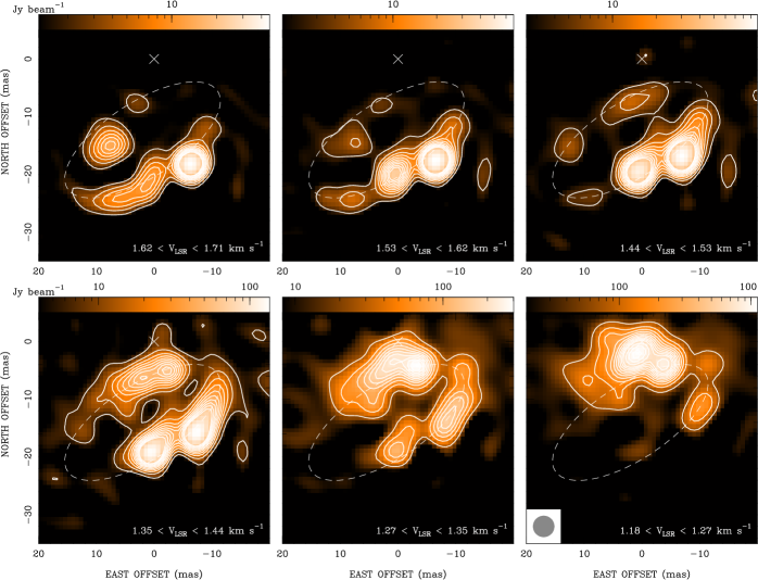
Figure 3: 6.7 GHz CH₃OH maser maps within $\sim 150$ AU south of the brightest CH₃OH maser (white cross). Each panel was obtained by summing the maser emission in three, consecutive, velocity channels (ranges in each bottom right corner). Contour levels start at 5 $\sigma$ and increase by 5 $\sigma$ steps for all panels but the two lower velocity maps which start at 10 $\sigma$ by 10 $\sigma$ steps. For each plot, the logarithmic color scale (upper wedge) range from a 3 $\sigma$ level up to the peak emission. The dashed ellipse marks the best fit to the overall maser emission. Restoring beam in the lower right panel.

All the methanol maser emission, except one faint feature, is projected within about 600 AU from the peak of component E 1 and spans more than three orders of magnitudes in brightness temperature, from $5\times 10^{8}$ to $2\times 10^{12}$ K. Individual CH₃OH cloudlets are grouped in two N-S filamentary structures to the east and west of the radio continuum peak E 1 (Figure 2) and cover a line-of-sight velocity range of 8 km s^-1. Emission from the strongest maser spots appears resolved in a core/halo morphology, as it is evidenced in Figure 3. Linewidths range between 0.17 and 0.36 km s^-1. Emission from the western filament is limited to negative LSR velocities, blueshifted with respect to the systemic velocity of the region, and its peak brightness temperature is less than $3\times 10^{10}$ K. The eastern filament includes the strongest, Galactic, 6.7 GHz CH₃OH maser feature, which is placed at zero offset in Figure 2. Its isotropic luminosity of $1\times 10^{-4}$ L_⊙ arises from a cloudlet with an apparent size of $\sim 30$ AU. Our observing epoch falls in the quiescent period between the 13th and 14th flare cycles on the basis of the ephemeris provided by Goedhart et al. (2003). Therefore, both values of brightness temperature and isotropic luminosity have to be taken as lower limits.

We note a quasi-elliptical distribution of CH₃OH maser emission which occurs within 150 AU to the south of the brightest maser feature (Figure 3). This emission is clearly detected within a V_LSR range of 0.5 km s^-1, at redshifted velocities with respect to the brightest maser. The ellipse is best fitted by a major axis of 31 mas, a minor axis of 13 mas, and a position angle of $-33\arcdeg$. If the apparent ellipticity were a projection of a circular ring in Keplerian rotation, viewed from an angle of $\sim 25\arcdeg$ from edge-on, the $0.25$ km s^-1 variation over a 16 mas radius would correspond to a central mass of $\rm 7\times 10^{-3}~{}M_{\odot}$. The central mass estimated from Keplerian rotation is about eight times that of Jupiter, which rules out a possible stellar system inside the ring.

4 DISCUSSION

The long-term monitoring performed with the HartRAO telescope by Goedhart et al. (2014, their Table 2) has set strong constraints on the periodic activity of the CH₃OH masers in G009.62+00.20 E. At 12.2 GHz, the periodic flaring has been detected at LSR velocities of 1.25, 1.64, and 2.12 km s^-1. At 6.7 GHz, the same flaring profile and recurrence are observed at 1.23, 1.84, 2.24, and 3.03 km s^-1. In Figure 2, we superpose the 12.2 GHz maser distribution by Sanna et al. (2009) with that at 6.7 GHz, by aligning the strongest maser features in both transitions. This alignment provides an optimal match between similar groups of features at 12.2 and 6.7 GHz, which also show LSR velocities in agreement within about 0.1 km s^-1. This evidence suggests that both maser lines arise from the same cloudlets. On the basis of VLBA observations of the 12.2 GHz maser emission during a flare, Goedhart et al. (2005) constrained the peak position of the flaring activity to within a few tens of mas from the strongest maser feature (at the origin of Figure 2). No significant flaring delays are detected among the 12.2 GHz features and between features at similar velocity in both maser transitions (Goedhart et al., 2014). After each flare event, the periodic masers decrease to the same brightness level they had before the flare, on a time scale of a few months.

As mapped with the LBA (Table 2), a number of 6.7 GHz maser cloudlets emit within the velocity range of the variable peak emission in the single-dish HartRAO spectra. This may suggest that the variable emission arises from a combination of different, bright, maser cloudlets, as well as possible extended emission resolved out on the long baselines. These cloudlets should have peak velocities within a maser linewidth from the variable single-dish peaks, in order to contribute significantly to the emission. By selecting these maser cloudlets in Table 2, we can confidently confine the region of periodic CH₃OH emission, including 12.2 GHz masers (Goedhart et al. 2005, their animated Figure 6), inside the solid box in Figure 2.

In recent years, three possible scenarios have been proposed to explain the periodic variability observed toward a number of Class II CH₃OH maser sources (Goedhart et al., 2014). The most recent one invokes stellar pulsation by a OB-type YSO in a pre zero-age-main-sequence (ZAMS) phase, under the assumption of accretion rates on the order of $\rm 10^{-3}~{}M_{\odot}~{}yr^{-1}$ (Inayoshi et al., 2013). This scenario does not apply to strong, photoionized, radio continuum sources as the model requires effective protostellar temperatures on the order of 5000 K. Two other models invoke the presence of a binary system of OB-type stars, which eventually provides the periodic modulation of either 1) the radiation field that is amplified by the maser (van der Walt, 2011), or 2) the IR radiation field that cause the population inversion of the maser levels (Araya et al., 2010). Model 1) requires the masing region amplifying a H ii continuum emission in the background, which is periodically enhanced by a colliding-wind binary (van der Walt, 2011, their Figure 1). Model 2) predicts the presence of a circumbinary disk which periodically accretes material onto a binary system, following simulations by Artymowicz & Lubow (1996), and periodically heats up a dusty envelope increasing the IR radiation field (see also a similar model by Parfenov & Sobolev 2014).

Currently, we cannot rule out a periodic variation of the radio continuum emission amplified by the maser cloudlets. If the source of input signal to the maser were coincident with component E 1, which is projected against the region of maser variability, maser cloudlets with different LSR velocities than the variable masers would likely lie further away from E 1. Otherwise, we make use of the YSO multiplicity, evidenced by the 7 mm continuum peaks, and the presence of high accretions rates ($\rm\sim 4\times 10^{-3}\,M_{\odot}\,yr^{-1}$) recently detected toward G009.62+00.20 E by Liu et al. (2011), to suggest that the maser variability may be explained by the superposition of two, independent, IR sources, which provide the pumping mechanism for Class II CH₃OH masers (Sobolev & Deguchi, 1994; Cragg et al., 2005). First, a constant IR radiation field provided by the warm dusty envelope associated with the radio continuum source E 1 (Figure 1). This environment would sustain the population inversion of the CH₃OH maser levels over the whole region and cause the maser emission during the quiescent flaring period. Second, an IR radiation field periodically enhanced by a growing massive YSO in the vicinity of the eastern CH₃OH maser distribution, following the model by Inayoshi et al. (2013). This object cannot be the main cause of radio continuum emission in the region. Instead, we consider an object associated with the faint radio component E 2, which lies (in projection) close to ($\sim 1000$ AU) the peak of the CH₃OH periodic activity.

To test this hypothesis, we compare the number of photons emitted by a warm dust layer surrounding source E 1, with those provided by the photosphere of a bloated protostar at the position of E 2. Assuming saturated masers, since the CH₃OH maser features increase by a factor up to 3 during the flaring period (Goedhart et al., 2014), these two sources of IR photons should be comparable. We consider a dust temperature on the order of 150 K (Cragg et al., 2005), consistent with the rotational temperature measured in the region from CH₃CN and H₂CS molecules (Hofner et al., 1996; Liu et al., 2011). For a frequency of about 13.5 THz, corresponding to the excitation of the upward links which pump the 12.2 GHz masers (Sobolev & Deguchi, 1994), we obtain a number of emitted photons per unit time and area (N_dust) of $\rm 1.7\times 10^{8}~{}s^{-1}~{}m^{-2}~{}Hz^{-1}$. We can parameterize the number of photons which effectively reaches a masing cloudlet, as a function of the relative distance of the the dust layer (R_dust) and the cloudlet (R_maser) with respect to the exciting YSO, $\rm 1.7\times 10^{8}\times(R_{dust}/R_{maser})^{2}~{}s^{-1}~{}m^{-2}~{}Hz^{-1}$. We then consider a secondary, variable, source of IR photons provided by a bloated protostar which pulsates at the period of the maser flares. Following eq. (3) of Inayoshi et al. (2013), this object would attain a protostellar radius of about 600 R_⊙, and a protostellar luminosity consistent with the IRAS fluxes measured in the region (e.g., Table 1 of Inayoshi et al. 2013). Such a protostar, with an effective temperature of 5000 K, would provide a number of 13.5 THz photons (N_proto) of $\rm 7\times 10^{5}~{}s^{-1}~{}m^{-2}~{}Hz^{-1}$ at the position of the periodic masers (box in Figure 2). Providing that the maser is saturated, we can reason on the position of the bloated protostar with respect to the masing gas. Assuming the bloated protostar at the position of E 2, the two pumping sources would be comparable if the masing cloudlets are observed in the foreground with respect to the warm dust layer (e.g., R${}_{maser}\sim 10\cdot R_{dust}$). Otherwise, the protostar should lie closer to ($<100$ AU) the region of periodic variability for R${}_{maser}\sim R_{dust}$.

A critical test for the presence of a pulsating protostar in the vicinity of the radio component E 2, may be provided by the eastern cluster of OH masers at a V_LSR of 1.65 km s^-1 (Figure 1). Since OH masers are radiatively pumped by an IR radiation field similar to the one exciting the Class II CH₃OH masers (Cragg et al., 2002), OH maser features close to the source of IR radiation may be subject to a similar periodic flaring as well, which would rule out model 1).

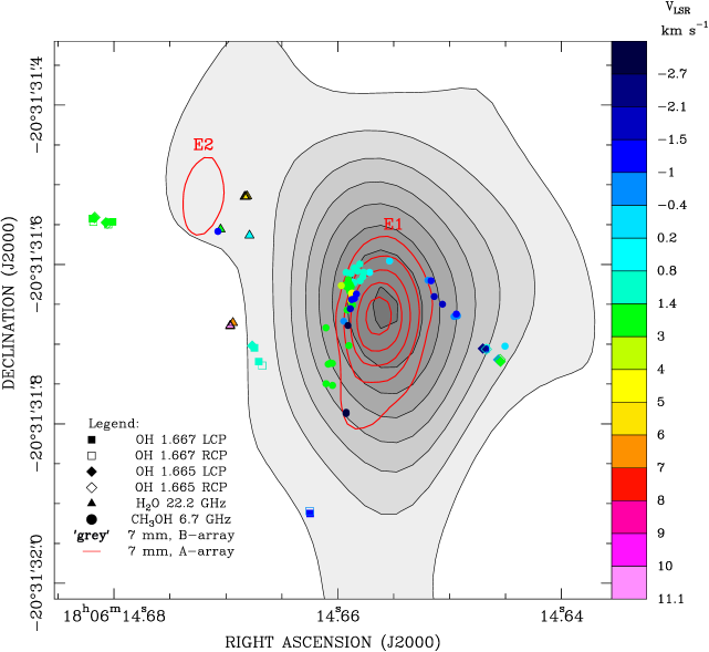
Figure 1: Combination of the VLBI measurements of different maser species obtained toward G009.62+00.20 E. The distribution of the maser cloudlets is superposed on the VLA maps at 7 mm, obtained with both the B and A configurations. Linear contouring was used for both maps starting from a 4 $\sigma$ level (Table 1); the first two negative levels fall below this threshold. Maser velocities along the line-of-sight are color coded according to the righthand V_LSR scale.

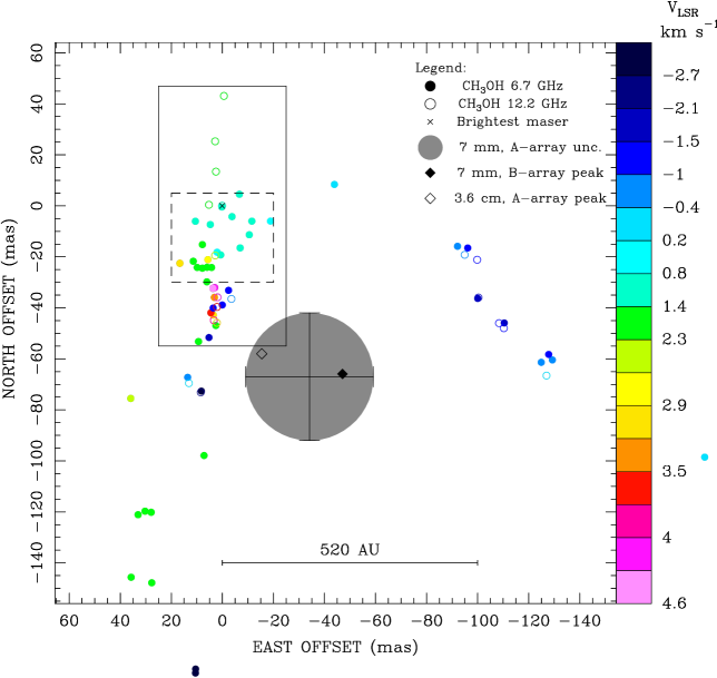
Figure 2: Close-up view of the 6.7 and 12.2 GHz (Sanna et al., 2009) maser emission arising within $\sim 600$ AU from the radio continuum peak. The 6.7 and 12.2 GHz masers are aligned by superposing their strongest features (cross) at zero offset. Maser velocities along the line-of-sight are color coded according to the righthand V_LSR scale. The large grey circle gives the astrometric uncertainty of the radio continuum peak. The solid and dashed boxes mark the region of maser variability, and that studied in Figure 3, respectively. Linear scale at the bottom.

Table 1: Observation and Source Information

							Peak position
Telescope	Band	exp.code	Obs.Date	Spec.Res.	HPBW	Image rms	R.A. (J2000)	Dec. (J2000)	Fpeak	Fint	VLSR
				(km s-1)	(mas)	(Jy beam-1)	(h m s)	($\arcdeg$ ’ ”)	(Jy beam-1)	(Jy)	(km s-1)
VLBA	L	BS224A	2013 Jul 02	0.18	$18\times 18$	0.03	18 06 14.6820	$-$20 31 31.542	21.15	30.12	1.65
LBA	C	V255A	2008 Mar 30	0.04	$3.7\times 3.7$	0.03	18 06 14.6586	$-$20 31 31.604	1010.63	3894.83	1.05
VLBA	K	BS208A	2012 Jan 19	0.21	$0.8\times 0.8$	0.01	18 06 14.6684	$-$20 31 31.515	0.78	1.10	-0.52
Radio Continuum
JVLA–A	Q	AS111	2011 Jun 16	…	$93\times 50$ at $-1.5\arcdeg$	$2\cdot 10^{-4}$	18 06 14.6562	$-$20 31 31.671	$5.6\cdot 10^{-3}$	$13.6\cdot 10^{-3}$	…
JVLA–B	Q	AG0685	2005 Feb/Apr	…	$284\times 163$ at $0.6\arcdeg$	$2\cdot 10^{-4}$	18 06 14.6555	$-$20 31 31.655	$6.9\cdot 10^{-3}$	$18.6\cdot 10^{-3}$	…

Note. — Columns 1 and 2 specify the interferometers and radio bands. Columns 3, 4, and 5 list the experiment code, observational epoch, and spectral resolution employed, respectively. Columns 6 and 7 give the restoring beam size and the rms noise of the final imaging. Columns 8 and 9 give the absolute position of the reference maser spots, and the peak position of the continuum emission. Columns 10 and 11 give the peak brightness and the flux density of the reference spots and the main continuum component determined by Gaussian fitting. Column 12 reports the LSR velocity of the reference spots.

Table 2: Parameters of maser features

Feature	VLSR	Fpeak	$\Delta\rm x$	$\Delta\rm y$
#	(km s-1)	(Jy beam-1)	(mas)	(mas)
OH features at 1.667 GHz – LCP
1	$1.65$	21.15	$0\pm 0.7$	$0\pm 0.2$
2	$2.01$	0.68	$-25.7\pm 0.5$	$-4.2\pm 1.7$
3	$-1.05$	0.62	$-273.8\pm 0.8$	$-370.3\pm 1.0$
4	$1.47$	0.31	$-203.8\pm 1.6$	$-162.4\pm 2.3$
5	$1.11$	0.27	$-209.2\pm 1.2$	$-179.7\pm 1.8$
6	$-1.59$	0.20	$-493.9\pm 2.7$	$-164.1\pm 2.1$
OH features at 1.667 GHz – RCP
7	$1.47$	2.06	$-1.5\pm 1.1$	$-4.2\pm 0.4$
8	$0.57$	1.39	$-494.7\pm 1.3$	$-163.1\pm 0.3$
9	$2.01$	0.53	$-20.1\pm 0.9$	$-7.4\pm 0.9$
10	$1.11$	0.39	$-213.7\pm 1.7$	$-184.8\pm 2.1$
11	$-0.69$	0.26	$-273.2\pm 1.2$	$-367.3\pm 1.3$
OH features at 1.665 GHz – LCP
12	$1.65$	10.01	$-2.9\pm 0.6$	$0.6\pm 0.5$
13	$1.83$	1.06	$-17.4\pm 2.0$	$-5.1\pm 2.0$
14	$-0.69$	0.86	$-510.0\pm 0.9$	$-177.2\pm 0.7$
15	$-2.32$	0.73	$-490.8\pm 0.5$	$-163.4\pm 0.8$
16	$2.01$	0.60	$-512.8\pm 1.0$	$-179.6\pm 1.8$
17	$1.29$	0.38	$-201.1\pm 1.3$	$-159.8\pm 1.3$
OH features at 1.665 GHz – RCP
18	$1.29$	5.00	$-495.1\pm 2.3$	$-164.1\pm 1.6$
19	$2.01$	4.35	$-512.3\pm 1.3$	$-177.1\pm 1.3$
20	$2.19$	2.73	$-19.1\pm 0.6$	$-6.2\pm 0.2$
21	$1.65$	2.17	$-3.4\pm 0.6$	$1.5\pm 0.5$
22.2 GHz H2O features
1	$-1.99$	1.05	$0.34\pm 0.07$	$0.03\pm 0.07$
2	$-0.52$	0.78	$0\pm 0.05$	$0\pm 0.03$
3	$3.06$	0.36	$-0.22\pm 0.15$	$-0.19\pm 0.12$
4	$6.22$	0.32	$14.99\pm 0.04$	$-158.11\pm 0.05$
5	$1.80$	0.30	$30.48\pm 0.03$	$-40.93\pm 0.07$
6	$7.70$	0.22	$18.43\pm 0.04$	$-162.34\pm 0.05$
7	$11.07$	0.17	$18.31\pm 0.04$	$-161.54\pm 0.09$
8	$4.75$	0.17	$-0.10\pm 0.08$	$-0.03\pm 0.12$
9	$6.01$	0.15	$-2.81\pm 0.11$	$0.67\pm 0.11$
10	$5.59$	0.11	$-1.50\pm 0.08$	$0.31\pm 0.13$
11	$0.54$	0.06	$-5.86\pm 0.09$	$-48.59\pm 0.15$
6.7 GHz CH3OH features
1	$1.05$	$1010.63$	$0\pm 0.54$	$0\pm 1.24$
2	$-0.45$	$565.03$	$13.50\pm 0.30$	$-67.26\pm 0.72$
3	$0.92$	$474.85$	$-6.76\pm 0.25$	$4.53\pm 0.54$
4	$1.18$	$347.72$	$-3.86\pm 0.80$	$-4.25\pm 0.36$
5	$1.13$	$80.94$	$-10.63\pm 0.44$	$-11.37\pm 0.32$
6	$1.13$	$69.66$	$10.47\pm 0.44$	$-6.07\pm 0.53$
7	$1.31$	$49.27$	$-7.06\pm 0.38$	$-16.51\pm 0.92$
8	$1.31$	$42.70$	$4.63\pm 0.22$	$-7.35\pm 0.07$
9	$1.40$	$41.58$	$0.57\pm 0.10$	$-19.27\pm 0.30$
10	$1.22$	$38.52$	$-11.65\pm 0.58$	$-6.02\pm 2.20$
11	$-1.06$	$31.90$	$-2.51\pm 0.33$	$-33.15\pm 0.21$
12	$2.98$	$30.90$	$3.46\pm 0.13$	$-42.85\pm 0.14$
13	$1.53$	$21.94$	$27.79\pm 0.34$	$-120.19\pm 0.17$
14	$0.17$	$17.21$	$-189.07\pm 0.14$	$-98.55\pm 0.13$
15	$3.68$	$14.88$	$4.39\pm 0.19$	$-41.96\pm 0.17$
16	$1.71$	$13.24$	$30.20\pm 0.44$	$-119.75\pm 0.14$
17	$-1.11$	$11.42$	$-96.23\pm 0.93$	$-16.53\pm 0.46$
18	$-0.89$	$11.22$	$-92.22\pm 0.25$	$-15.88\pm 0.27$
19	$4.60$	$9.21$	$3.61\pm 0.13$	$-32.36\pm 0.26$
20	$-2.12$	$8.94$	$-100.14\pm 0.14$	$-36.31\pm 0.22$
21	$0.78$	$8.25$	$-18.97\pm 0.22$	$-6.01\pm 0.18$
22	$2.80$	$7.67$	$5.57\pm 0.05$	$-21.12\pm 0.06$
23	$-1.63$	$6.77$	$-110.54\pm 0.40$	$-45.94\pm 0.32$
24	$3.16$	$6.77$	$3.03\pm 0.18$	$-35.91\pm 0.19$
25	$1.49$	$6.69$	$32.92\pm 0.16$	$-121.14\pm 0.15$
26	$-0.62$	$6.21$	$-125.04\pm 0.27$	$-61.38\pm 0.45$
27	$0.70$	$5.45$	$1.96\pm 0.09$	$-18.21\pm 0.12$
28	$1.71$	$5.43$	$7.74\pm 0.20$	$-15.22\pm 0.18$
29	$-1.46$	$5.22$	$-0.06\pm 0.19$	$-38.88\pm 0.36$
30	$-1.55$	$4.99$	$3.52\pm 0.21$	$-40.09\pm 0.11$
31	$1.84$	$4.28$	$35.66\pm 0.15$	$-145.66\pm 0.15$
32	$2.15$	$3.93$	$2.46\pm 0.30$	$-46.93\pm 0.23$
33	$1.53$	$3.79$	$7.09\pm 0.17$	$-97.93\pm 0.19$
34	$1.75$	$3.72$	$4.15\pm 0.23$	$-24.19\pm 0.37$
35	$1.66$	$2.85$	$5.91\pm 0.21$	$-24.12\pm 0.12$
36	$4.08$	$2.83$	$2.93\pm 0.12$	$-32.09\pm 0.16$
37	$1.62$	$2.78$	$7.74\pm 0.29$	$-24.47\pm 0.14$
38	$3.02$	$2.21$	$16.56\pm 0.15$	$-22.54\pm 0.18$
39	$1.53$	$2.07$	$9.77\pm 0.53$	$-24.18\pm 0.26$
40	$-1.37$	$1.73$	$-127.95\pm 0.17$	$-58.28\pm 0.17$
41	$2.32$	$1.41$	$11.30\pm 0.24$	$-21.75\pm 0.14$
42	$-0.93$	$1.33$	$-129.40\pm 0.33$	$-60.45\pm 0.30$
43	$2.19$	$1.33$	$5.98\pm 0.29$	$-29.82\pm 0.35$
44	$1.88$	$1.09$	$27.57\pm 0.23$	$-147.83\pm 0.21$
45	$2.23$	$0.96$	$9.26\pm 0.31$	$-53.23\pm 0.39$
46	$-1.50$	$0.95$	$171.49\pm 0.63$	$45.45\pm 0.76$
47	$0.04$	$0.85$	$-43.98\pm 0.41$	$8.37\pm 0.18$
48	$-1.76$	$0.62$	$5.16\pm 0.21$	$-51.65\pm 0.23$
49	$-3.30$	$0.56$	$8.15\pm 0.25$	$-72.68\pm 0.30$
50	$2.50$	$0.47$	$35.80\pm 0.29$	$-75.53\pm 0.24$
51	$-2.82$	$0.33$	$10.44\pm 0.41$	$-183.21\pm 0.46$
52	$-3.04$	$0.32$	$10.39\pm 0.29$	$-181.65\pm 0.38$

Note. — Maser features detected within $1^{\prime\prime}$ from G009.62+00.20 E listed by decreasing brightness (Column 1). OH maser features are listed for each circular polarization component. Columns 2 and 3 report the LSR velocity and brightness of the brightest spot of each feature. Columns 5 and 6 give the relative centroid position of each feature in the east and north directions, respectively. Reference absolute positions are reported in Table 1. The uncertainties give the intensity-weighted standard deviation of the spots’ distribution within a given feature.

References

- Araya et al. (2010) Araya, E. D., Hofner, P., Goss, W. M., et al. 2010, ApJ, 717, L133
- Artymowicz & Lubow (1996) Artymowicz, P., & Lubow, S. H. 1996, ApJ, 467, L77
- Cragg et al. (2002) Cragg, D. M., Sobolev, A. M., & Godfrey, P. D. 2002, MNRAS, 331, 521
- Cragg et al. (2005) Cragg, D. M., Sobolev, A. M., & Godfrey, P. D. 2005, MNRAS, 360, 533
- Deller et al. (2007) Deller, A. T., Tingay, S. J., Bailes, M., & West, C. 2007, PASP, 119, 318
- Fish et al. (2005) Fish, V. L., Reid, M. J., Argon, A. L., & Zheng, X.-W. 2005, ApJS, 160, 220
- Franco et al. (2000) Franco, J., Kurtz, S., Hofner, P., et al. 2000, ApJ, 542, L143
- Garay et al. (1993) Garay, G., Rodriguez, L. F., Moran, J. M., & Churchwell, E. 1993, ApJ, 418, 368
- Goedhart et al. (2003) Goedhart, S., Gaylard, M. J., & van der Walt, D. J. 2003, MNRAS, 339, L33
- Goedhart et al. (2005) Goedhart, S., Minier, V., Gaylard, M. J., & van der Walt, D. J. 2005, MNRAS, 356, 839
- Goedhart et al. (2014) Goedhart, S., Maswanganye, J. P., Gaylard, M. J., & van der Walt, D. J. 2014, MNRAS, 437, 1808
- Hofner et al. (1994) Hofner, P., Kurtz, S., Churchwell, E., Walmsley, C. M., & Cesaroni, R. 1994, ApJ, 429, L85
- Hofner & Churchwell (1996) Hofner, P., & Churchwell, E. 1996, A&AS, 120, 283
- Hofner et al. (1996) Hofner, P., Kurtz, S., Churchwell, E., Walmsley, C. M., & Cesaroni, R. 1996, ApJ, 460, 359
- Hofner et al. (2001) Hofner, P., Wiesemeyer, H., & Henning, T. 2001, ApJ, 549, 425
- Inayoshi et al. (2013) Inayoshi, K., Sugiyama, K., Hosokawa, T., Motogi, K., & Tanaka, K. E. I. 2013, ApJ, 769, L20
- Linz et al. (2005) Linz, H., Stecklum, B., Henning, T., Hofner, P., & Brandl, B. 2005, A&A, 429, 903
- Liu et al. (2011) Liu, T., Wu, Y., Liu, S.-Y., et al. 2011, ApJ, 730, 102
- Minier et al. (2002) Minier, V., Booth, R. S., & Conway, J. E. 2002, A&A, 383, 614
- Sobolev & Deguchi (1994) Sobolev, A. M., & Deguchi, S. 1994, A&A, 291, 569
- Menten (1991) Menten, K. M. 1991, ApJ, 380, L75
- Parfenov & Sobolev (2014) Parfenov, S. Y., & Sobolev, A. M. 2014, MNRAS, 444, 620
- Persi et al. (2003) Persi, P., Tapia, M., Roth, M., et al. 2003, A&A, 397, 227
- Petrov et al. (2006) Petrov, L., Kovalev, Y. Y., Fomalont, E. B., & Gordon, D. 2006, AJ, 131, 1872
- Phillips et al. (1998) Phillips, C. J., Norris, R. P., Ellingsen, S. P., & McCulloch, P. M. 1998, MNRAS, 300, 1131
- Reid (1995) Reid, M. J. 1995, Very Long Baseline Interferometry and the VLBA, 82, 209
- Reid et al. (2009) Reid, M. J., Menten, K. M., Brunthaler, A., Zheng, X. W., Moscadelli, L., & Xu, Y. 2009, ApJ, 693, 397
- Sanna et al. (2009) Sanna, A., Reid, M. J., Moscadelli, L., et al. 2009, ApJ, 706, 464
- Sanna et al. (2010) Sanna, A., Moscadelli, L., Cesaroni, R., Tarchi, A., Furuya, R. S., & Goddi, C. 2010, A&A, 517, A71
- Sanna et al. (2014) Sanna, A., Reid, M. J., Menten, K. M., et al. 2014, ApJ, 781, 108
- Testi et al. (2000) Testi, L., Hofner, P., Kurtz, S., & Rupen, M. 2000, A&A, 359, L5
- van der Walt et al. (2009) van der Walt, D. J., Goedhart, S., & Gaylard, M. J. 2009, MNRAS, 398, 961
- van der Walt (2011) van der Walt, D. J. 2011, AJ, 141, 152