Approximate Joint MAP Detection
of Co-Channel Signals

Abstract

We consider joint detection of co-channel signals—specifically, signals which do not possess a natural separability due to, for example, the multiple access technique or the use of multiple antennas. Iterative joint detection and decoding is a well known approach for utilizing the error correction code to improve detection performance. However, the joint maximum a posteriori probability (MAP) detector may be prohibitively complex, especially in a multipath channel. In this paper, we present an approximation to the joint MAP detector motivated by a factor graph model of the received signal. The proposed algorithm is designed to approximate the joint MAP detector as closely as possible within the computational capability of the receiver.

I Introduction

Detection of a desired signal in the presence of one or more interfering signals is a prevalent problem in dense wireless communication systems. As a result, designing receivers capable of detection in the presence of interference has been a very active area of research with numerous algorithms proposed in literature. Iterative multiuser detection problems have been considered for code division multiple access (CDMA) [1, 2], spatial multiplexing [3, 4, 5], and multiuser MIMO [6, 7], among others. Receiver algorithms generally fit into one of three categories: linear filtering, interference cancellation, and joint detection.

Linear filtering may be applied in the time, space, or space-time dimension(s) and includes techniques such as matched filtering, minimum mean square error (MMSE) equalization, and beamforming. In systems which employ spreading sequences or multiple antennas, linear filtering can be an effective means of interference mitigation, specifically when the spreading gain or number of antennas is greater than or equal to the number of signals present.

Interference cancellation refers to algorithms in which each user’s signal is canceled from the received signal after detection (e.g., [8, 9] and the references therein). Linear filtering combined with interference cancellation may further improve detection and has been a very successful approach for spatial multiplexing [10]. Soft cancellation in conjunction with soft decoding of the channel code—often referred to as “turbo” interference cancellation—has been shown to achieve good results in a CDMA system [1].

Optimal maximum a posteriori probability (MAP) detection is performed by jointly detecting both the desired and co-channel signals. The detection stage is separated from decoding and probabilistic information is passed between the joint MAP detector and a collection of single user decoders. The separation of detection and decoding is justified by message passing algorithms which operate on a factor graph of the joint probability density function [11]. Yet, even with the separation of detection and decoding, joint MAP detection may be prohibitively complex as a result of high-order modulations, numerous users, or inter-symbol interference (ISI).

A challenging case is detection in the presence of non-orthogonal, asynchronous interfering signals using a single receive antenna. That is, reception of co-channel signals which do not possess a natural separability due to a multiple access technique (such as CDMA) or multiple antennas. As a result, linear filtering and interference cancellation are ineffective especially when the signal power levels are similar.

Joint MAP detection in such a signal model is developed and studied in [12]. The separability is achieved due to both frame and symbol timing offsets and an error correction code. Joint detection which accounts for the strongest ISI terms is proposed. Thus, the algorithm is exponentially complex in the number of co-channel signals. For this reason its application is limited to 2 users and BPSK modulation in [12]. A large number of users or high-order modulations in addition to ISI due to the asynchronous signals makes the optimal joint MAP detector extremely complex.

Jiang and Li consider single antenna interference cancellation in a frequency selective, multiple access channel [13]. The same channel code, interleaver, and modulation is assumed for all co-channel signals. Signal separability is obtained through the independence of each user’s multipath channel. Jiang and Li propose a concurrent MAP (CMAP) algorithm in which a Gaussian approximation is used for co-channel interference and MAP equalization for ISI. The CMAP algorithm is compared to joint MAP detection, the Rake Gaussian method proposed in [14], and soft interference cancellation with MAP equalization. While the CMAP algorithm is the state-of-the-art in addressing the difficult detection problem described above, performance is degraded when the Gaussian approximation is made for strong co-channel interference terms.

In this paper, we present a new approximation to the joint MAP detector which is motivated by a factor graph model of the received signal. The proposed algorithm is designed to approximate the joint MAP detector as closely as possible within the computational capability of the receiver. The complexity of the algorithm is adjustable and can be set to account for the capabilities of the receiver, the desired performance, or the difficulty of the detection task.

The paper is organized as follows. The system model is presented in Section II followed by development of the MAP detector in Section III. The complexity of the proposed algorithm is compared with algorithms from the literature in Section IV and a detailed description of the proposed algorithm is provided in Section V. The algorithms are compared via simulation in Section VI and conclusions are drawn in Section VII.

Notation

Let $\mathbf{x}$ denote a column vector $\mathbf{x}=[x_{0},\ldots,x_{K-1}]^{\mathrm{T}}$. We use the shorthand $\sum_{x_{k}}$ to denote the summation over the domain of $x_{k}$. Similarly, $\sum_{\mathbf{x}}$ denotes the summation over the domain of the vector $\mathbf{x}$ and $\sum_{\mathbf{x}\backslash x_{k}}$ denotes the summation with respect to all variables except $x_{k}$.

II System Model

In this work we consider single antenna reception of $U$ co-channel signals (users). Let the information bits, coded bits, and symbols of the $u$th user be denoted by column vectors $\mathbf{b}^{(u)}$, $\mathbf{c}^{(u)}$, and $\mathbf{x}^{(u)}$, respectively. We define the collection of these terms for all users as

$$\mathbf{B}=[\mathbf{b}^{(1)},\ldots,\mathbf{b}^{(U)}]$$

$$\mathbf{C}=[\mathbf{c}^{(1)},\ldots,\mathbf{c}^{(U)}]$$

$$\mathbf{X}=[\mathbf{x}^{(1)},\ldots,\mathbf{x}^{(U)}].$$

The $n$th sample of the received signal is given by

$$r_{n}=\sum_{u=1}^{U}\sum_{l=0}^{L-1}h_{l}^{(u)}x_{n-l}^{(u)}+w_{n},$$ (1)

where $\mathbf{h}^{(u)}=[h_{0}^{(u)},h_{1}^{(u)},\ldots,h_{L-1}^{(u)}]^{\mathrm{T}}$ denotes the combined effect of the multipath channel and the transmit pulse for the $u$th user, $L$ is the number of channel taps, and $\{w_{n}\}_{n=0}^{N-1}$ are independent and identically distributed circularly-symmetric complex Gaussian random variables with variance $\sigma^{2}$. The collection of all received samples is denoted $\mathbf{r}=[r_{0},\ldots,r_{N-1}]$. In general the transmitted signals may be symbol-asynchronous. For the sake of notational simplicity, the model provided in (1) makes a number of assumptions about the received signal—for example, that the channel duration of the users $L$ is identical and that the received signal is sampled at a single sample per symbol. However, the multiuser detection and equalization algorithms presented in this paper are applicable to the more general cases.

III MAP Detection

The goal of the receiver is to detect all information bits $\mathbf{B}$ given observation $\mathbf{r}$. Because of the complexity of sequence detection of $\mathbf{B}$, we desire to perform MAP symbol-by-symbol (in our case, bit-by-bit) detection. The detector for the $k$th bit of user $u$ is given by

$$\hat{b}_{k}^{(u)}=\operatorname*{arg\,max}_{b_{k}^{(u)}}\sum_{\mathbf{B}\backslash b_{k}^{(u)}}{p(\mathbf{B}|\mathbf{r})},$$ (2)

where the marginal is computed for $b_{k}^{(u)}$. According to Bayes’ rule, (2) is equivalent to

$$\hat{b}_{k}^{(u)}=\operatorname*{arg\,max}_{b_{k}^{(u)}}\sum_{\mathbf{B}\backslash b_{k}^{(u)}}{f(\mathbf{r},\mathbf{B})},$$ (3)

where the term $1/f(\mathbf{r})$ is a constant which has been removed. By the Total Probability Theorem, (3) can further be expressed as a marginalization over the full joint distribution as given by

$$\hat{b}_{k}^{(u)}=\operatorname*{arg\,max}_{b_{k}^{(u)}}\sum_{\mathbf{X},\mathbf{C},\mathbf{B}\backslash b_{k}^{(u)}}{f(\mathbf{r},\mathbf{X},\mathbf{C},\mathbf{B})}.$$ (4)

The marginalization in (4) cannot be performed directly, but an iterative implementation of the sum-product algorithm is well suited for this task.

III-A Probability Distribution

Taking into account conditional independence of the variables, the joint distribution is given by

$$f(\mathbf{r},\mathbf{X},\mathbf{C},\mathbf{B})= \prod_{n=0}^{N-1}f(r_{n}|\mathbf{x}^{(1)},\ldots,\mathbf{x}^{(U)})$$

$$\prod_{u=1}^{U}{p(\mathbf{x}^{(u)}|\mathbf{c}^{(u)})p(\mathbf{c}^{(u)}|\mathbf{b}^{(u)})p(\mathbf{b}^{(u)})}.$$ (5)

Factorizations of the modulation $p(\mathbf{x}^{(u)}|\mathbf{c}^{(u)})$ and code $p(\mathbf{c}^{(u)}|\mathbf{b}^{(u)})$ constraints have been explored in the literature (see, for example, [11, 15]). From (1) the likelihood function for each term $r_{n}$ is dependent on a subset of the symbols. We define, $\mathbf{x}_{[n]}^{(u)}=[x_{n-L+1}^{(u)},\ldots,x_{n}^{(u)}]^{\mathrm{T}}$ to denote the symbols from user $u$ which have components in the $r_{n}$ sample. The distribution is then given by

$$f(\mathbf{r},\mathbf{X},\mathbf{C},\mathbf{B})= \prod_{n=0}^{N-1}f(r_{n}|\mathbf{x}_{[n]}^{(1)},\ldots,\mathbf{x}_{[n]}^{(U)})$$

$$\prod_{u=1}^{U}{p(\mathbf{x}^{(u)}|\mathbf{c}^{(u)})p(\mathbf{c}^{(u)}|\mathbf{b}^{(u)})p(\mathbf{b}^{(u)})}.$$ (6)

Soft output MAP equalization of an ISI channel may be accomplished via the BCJR algorithm [16]. This algorithm was extended to the case of joint detection of a desired and co-channel signal in ISI by Moon and Gunther [12]. The algorithm relies on the introduction of state variables $\mathbf{m}_{0},\ldots,\mathbf{m}_{N}$ into the likelihood function as follows:

$$\prod_{n=0}^{N-1}f(r_{n}|\mathbf{x}_{[n]}^{(1)},\ldots,\mathbf{x}_{[n]}^{(U)})$$

$$\qquad=\prod_{n=0}^{N-1}\sum_{\mathbf{m}_{n}}f(r_{n},\mathbf{m}_{n+1}|x_{n}^{(1)},\ldots,x_{n}^{(U)},\mathbf{m}_{n})p(\mathbf{m}_{0})$$ (7)

where $\mathbf{m}_{n}=[x_{n-L+1}^{(1)},\ldots,x_{n-1}^{(1)},\ldots,x_{n-L+1}^{(U)},\ldots,x_{n-1}^{(N)}]^{\mathrm{T}}$.

At a high level, local marginals for the symbols are computed by a forward and backward pass of the BCJR algorithm (also known as the forward-backward algorithm). The forward messages are given by

$$\alpha(\mathbf{m}_{i+1})=\prod_{n=0}^{i}\sum_{\mathbf{m}_{n}}f(r_{n},\mathbf{m}_{n+1}|x_{n}^{(1)},\ldots,x_{n}^{(U)},\mathbf{m}_{n})p(\mathbf{m}_{0})$$ (8)

and

$$\beta(\mathbf{m}_{i})=\prod_{n=i}^{N-1}\sum_{\mathbf{m}_{n+1}}f(r_{n},\mathbf{m}_{n+1}|x_{n}^{(1)},\ldots,x_{n}^{(U)},\mathbf{m}_{n}).$$ (9)

The messages may be defined recursively as given by

$$\alpha(\mathbf{m}_{i+1})=\sum_{\mathbf{m}_{i}}\gamma(\mathbf{m}_{i+1},\mathbf{m}_{i})\alpha(\mathbf{m}_{i})$$ (10)

and

$$\beta(\mathbf{m}_{i})=\sum_{\mathbf{m}_{i+1}}\gamma(\mathbf{m}_{i+1},\mathbf{m}_{i})\beta(\mathbf{m}_{i+1}),$$ (11)

where $\gamma(\mathbf{m}_{i+1},\mathbf{m}_{i})=f(r_{i},\mathbf{m}_{i+1}|x_{i}^{(1)},\ldots,x_{i}^{(U)},\mathbf{m}_{i})$, $\alpha(\mathbf{m}_{0})=p(m_{0})=1$, and $\beta(\mathbf{m}_{N})=1$. A marginal for a particular symbol $x_{i}^{(u)}$ is given by $\sum_{x_{[i]}^{(1)},\ldots,x_{[i]}^{(U)}\backslash x_{i}^{(u)}}\alpha(\mathbf{m}_{i})\gamma(\mathbf{m}_{i},\mathbf{m}_{i+1})\beta(\mathbf{m}_{i+1})$. The joint MAP detector is developed for the case of a received signal with two samples per symbol in [12].

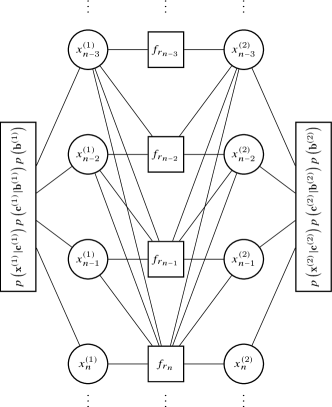
Figure 1: Factor graph of $f(\mathbf{r},\mathbf{X},\mathbf{C},\mathbf{B})$ for $U=2$ and $L=4$ based on the factorization in (6).

Figure 2: Factor graph of $f(\mathbf{r},\mathbf{X},\mathbf{C},\mathbf{B})$ for $U=2$ and $L=4$ based on the state space model factorization of (7) substituted into (6).

III-B Factor Graph Model

The sum-product algorithm performs efficient marginalization by exploiting the factorization of the joint distribution $f(\mathbf{r},\mathbf{X},\mathbf{C},\mathbf{B})$. As an example, consider the case of $U=2$ and $L=4$. The factor graph of the joint distribution in (6) is given in Fig. 1. Similarly, the factor graph of the joint distribution with the introduction of the state variables is shown in Fig. 2. In Fig. 1, $f_{r_{n}}$ denotes the factor $f(r_{n}|\mathbf{x}_{[n]}^{(1)},\mathbf{x}_{[n]}^{(2)})$ and, in Fig. 2, $f_{r_{n}}$ denotes the factor $f(r_{n},\mathbf{m}_{n+1}|x_{n}^{(1)},\ldots,x_{n}^{(U)},\mathbf{m}_{n})$. We refer to the factor graphs in Fig. 1 and 2 as the fully connected graph and the state-space model (SSM) graph, respectively.

The generalization of the BCJR algorithm to the factor graph of the joint distribution is given by the sum-product algorithm [15]. The factor nodes $p(\mathbf{x}^{(u)}|\mathbf{c}^{(u)})p(\mathbf{c}^{(u)}|\mathbf{b}^{(u)})p(\mathbf{b}^{(u)})$ are further factored when implementing the sum-product algorithm. The factor nodes related to the observations $f_{r_{n}}$ and the symbol variable nodes make up the “detection block” of the factor graph. The fully connected graph contains cycles within the detection block; the SSM graph eliminates these cycles. Cycles have a negative impact on the convergence of the sum-product algorithm. In Section V, we develop an algorithm to reduce the complexity of joint MAP detection based on the fully connected factor graph of Fig. 1. In Section VI, we quantify the loss in performance when performing message passing on the fully connected graph versus the SSM graph.

IV Complexity

For both graphs, the complexity associated with each of the detection factor nodes is $\mathcal{O}(M^{UL})$ where $M$ is the modulation order of the symbols (assumed to be the same for each user). The complexity is exponential in the number of users and channel taps and therefore complexity prohibits use of the joint MAP detector in many potential co-channel signal scenarios. Specifically when either $M>>2$, $U>>2$, or $L>>2$ and especially when this is the case for two of these terms. As an example, the complexity for QPSK, 4 users, and 4 channel taps (i.e., $M=4$, $U=4$, and $L=4$) is $\mathcal{O}(10^{9})$.

Because of the problem of complexity with joint MAP detector, approaches with lower complexity have been considered for this problem.

• Interference Cancellation: Cancellation may be performed based on either hard or soft decisions. Detection is performed starting with the strongest signal and continuing to the weakest. Soft cancellation may be combined with iterative processing to iteratively improve the soft estimates.

• Rake Gaussian: This method was proposed in [14] for interleave-division multiple access. In this method, for the detection of symbol $x_{k}^{(u)}$ all other symbols are modeled as Gaussian random variables. This includes the symbols of all other users and all other symbols of the desired user, i.e., $\{x_{k^{\prime}}^{(u^{\prime})}\}_{u^{\prime}\neq u,k^{\prime}\neq k}$. The mean and variance of the Gaussian distribution are computed from the extrinsic symbol probabilities obtained from demodulation and decoding.

• Concurrent MAP (CMAP): This method was proposed in [13] to improve upon the performance of the Rake Gaussian method. In this method, MAP equalization of each user’s signal is performed while all other user’s signals are modeled as Gaussian random variables. Thus, the complexity of the method is $\mathcal{O}(U\cdot M^{L})$, that is, linear in the number of users and exponential in the number of channel taps.

Visual comparisons of the Rake Gaussian and CMAP algorithms are given using factor graphs. The factor node $f_{r_{3}}$ from the example in Fig. 1 is used to represent the approximations made by the Rake Gaussian and CMAP algorithms when computing the message $m_{f_{r_{3}}\rightarrow x_{2}^{(1)}}$ in Figs. 3 and 4, respectively. The single arrow represent messages containing discrete distributions and the double arrow represent messages which contain a mean and variance based on a Gaussian approximation.

The graphical models of Figs. 3 and 4 motivate a new approach in which the distribution of weaker terms in the signal component of $r_{n}$ are modeled as Gaussian random variables. Sum-product message passing is performed for the stronger terms in $r_{n}$. This hybrid approach has a complexity determined by the number of messages with discrete distributions and maintains a single, connected graph. The graphical model for the hybrid approach is shown in Fig. 5 where symbols $x_{1}^{(1)}$, $x_{2}^{(1)}$, $x_{1}^{(2)}$, and $x_{2}^{(2)}$ are the strongest component in $r_{3}$ for users 1 and 2 (i.e., the power of the channel coefficient $|h_{l}^{(u)}|^{2}$ is strongest for these terms). This model is motivated by common transmit pulse shapes which contain the majority of their energy within the center of the pulse and multipath channels which often exhibit an exponential decay. A detailed description of the algorithm is provided in the following section.

Figure 3: Factor graph motivated representation of the Rake Gaussian method.

Figure 4: Factor graph motivated representation of the CMAP method. As shown, this factor is a slice of the overall graph to implement MAP equalization of user 1 while modeling the interference from user 2.

Figure 5: Factor graph motivated representation of the approximate MAP method developed in this work.

V Approximate MAP Detection Algorithm

Consider a generic interference model (to represent inter-symbol interference, co-channel interference, or both) in which $K$ signal components $x_{1},x_{2},\ldots,x_{K}$ are received with channel coefficients $h_{1},h_{2},\ldots,h_{K}$, respectively. The received signal is given by

$$y=\sum_{k=1}^{K}h_{k}x_{k}+w$$

where $y$ represents one sample of a larger sequence of received samples and the noise $w$ is modeled as a circularly symmetric complex Gaussian random variable with variance $\sigma^{2}$. The factor associated with the received sample $y$ is given by

$$f(y|x_{1},\ldots,x_{K})=\mathcal{CN}\Biggl{(}y;\sum_{k=1}^{K}h_{k}x_{k}\,,\,\sigma^{2}\Biggr{)}$$

where the channel coefficients and the noise power $\sigma^{2}$ are assumed to be known.

The message from factor node $f_{y}$ to variable node $x_{k}$ is denoted $m_{f_{y}\rightarrow x_{k}}$. Similarly, the message from variable node $x_{k}$ to factor node $f_{y}$ is denoted $n_{x_{k}\rightarrow f_{y}}$. According to the sum-product algorithm, the message $m_{f_{y}\rightarrow x_{i}}$ is given by

$$m_{f_{y}\rightarrow x_{i}}(x_{i})=\sum_{\mathbf{x}\backslash x_{i}}f(y|x_{1},\ldots,x_{K})\prod_{k\neq i}n_{x_{k}\rightarrow f_{y}}(x_{k}).$$ (12)

The proposed algorithm modifies the sum-product algorithm computations as follows:

• The mean and variance of the input messages are computed according to

  $$\mu_{x_{k}}=\sum_{x_{k}}x_{k}n_{x_{k}\rightarrow f_{y}}(x_{k})$$

  $$\sigma_{x_{k}}^{2}=\sum_{x_{k}}|x_{k}-\mu_{x_{k}}|^{2}n_{x_{k}\rightarrow f_{y}}(x_{k})$$

  for all $k=1,\ldots,K$.

• For computation of the outgoing message $m_{f_{y}\rightarrow x_{i}}(x_{i})$, the remaining variables for $k\neq i$ are sorted by their channel coefficient power $|h_{k}|^{2}$. Let the set $\mathcal{A}$ index the variables associated with the strongest channel coefficients. These variables remain a part of the local marginalization as given in (12). The number of variables in the set $\mathcal{A}$ will depend on the acceptable complexity in implementation. The indices of the weaker components are included in the set $\mathcal{B}$ and the distributions of these variables are approximated by Gaussian random variables to eliminate the marginalization over these variables. Let the variables associated with sets $\mathcal{A}$ and $\mathcal{B}$ be given by $\mathbf{x}_{\mathcal{A}}$ and $\mathbf{x}_{\mathcal{B}}$, respectively.

• The message is computed with the following approximate sum-product computation:

  $$m_{f_{y}\rightarrow x_{i}}(x_{i})=\sum_{\mathbf{x}_{\mathcal{A}}}\tilde{f}(y|x_{i},\mathbf{x}_{\mathcal{A}})\prod_{k\in\mathcal{A}}n_{x_{k}\rightarrow f_{y}}(x_{k})$$

  where

$$\tilde{f}(y|x_{i},\mathbf{x}_{\mathcal{A}})=$$

$$\mathcal{CN}\Biggl{(}y;h_{i}x_{i}+\sum_{k\in\mathcal{A}}h_{k}x_{k}+\sum_{l\in\mathcal{B}}h_{l}\mu_{x_{l}}\,,\,\sigma^{2}+\sum_{l\in\mathcal{B}}|h_{l}|^{2}\sigma_{x_{l}}^{2}\Biggr{)}.$$ (13)

This algorithm is applied to the computation of the sum-product messages at each of the detection factors in Fig. 1. The complexity of the proposed algorithm for each factor is $\mathcal{O}(UL\cdot M^{|\mathcal{A}|+1})$ where $|\mathcal{A}|$ is the number of symbols included in the set $\mathcal{A}$. Thus, by choosing the size of $\mathcal{A}$, the complexity of the algorithm may be adjusted to match the computational capability of the receiver and performance requirements.

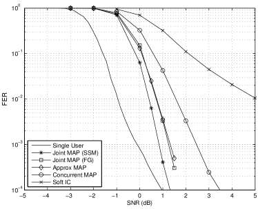
Figure 6: FER comparison of the joint MAP state-space model (Joint MAP (SSM)), the joint MAP fully connected factor graph (Joint MAP (FG)), the proposed approximate MAP algorithm (Approx MAP), CMAP (Concurrent MAP), and soft interference cancellation (Soft IC) algorithms with SIR=0 dB.

VI Numerical Results

We first simulate the performance for a scenario in line with the one considered in [12]: two users ($U=2$) each employing BPSK modulation ($M=2$). ISI results from symbol timing offsets between the users and a transmit pulse with a duration of four symbol periods ($L=4$). The selection of these parameters allows us to simulate the joint MAP detector for the purpose of comparison. The simulation parameters are summarized as follows:

• Code: 1/2-rate turbo code with 500 coded bits

• Modulation: BPSK

• Pulse: Square root raised cosine with $L=4$ and roll-off factor 0.35

• A relative time delay between the users of $T/4$ is chosen where $T$ is the symbol period

• A relative phase offset between the channel coefficients of the users of $\pi/6$ is chosen

• 15 iterations of message passing are performed

The FER performance is shown in Fig. 6 for the joint MAP (with the SSM and fully connected factor graphs), the proposed novel approach, CMAP, and soft interference cancellation algorithms. The approximate MAP algorithm is implemented with $|\mathcal{A}|=3$. Thus, the proposed approximate MAP algorithm and the CMAP algorithm have the same order of complexity (per iteration). The performance of the fully connected factor graph demonstrates a loss of about 0.5 dB compared to the SSM factor graph. The proposed approximate MAP algorithm is based on the fully connected graph and we observe that it achieves nearly identical performance to the receiver which uses exact sum-product computations. At a FER of $10^{-3}$ the proposed approximate MAP approach and Concurrent MAP approach demonstrate losses of 0.5 dB and 1.5 dB, respectively, compared to joint MAP detection based on the SSM. We observe that the Soft IC method becomes limited by interference as signal-to-noise ratio (SNR) increases.

We also consider a 2-user scenario with QPSK modulation with a 4-tap multipath channel. The average power in each multipath component is given by $[0.644,0.237,0.087,0.032]$. In Fig. 7 the FER of the proposed approximate MAP algorithm and the CMAP algorithm is shown. Both SNR and signal-to-interference ratio (SIR) are computed with respect to the instantaneous power in the multipath channel. The most significant improvement in FER is achieved by the proposed approximate MAP algorithm when the signals have similar power levels ($-3\leq\text{SIR}\leq 3$ dB) and the SNR is high.

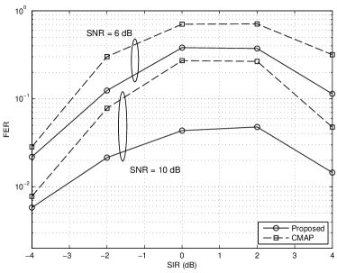
Figure 7: FER of the proposed and CMAP algorithms with respect to SIR. Both signals are detected, and the FER of the desired signal is shown. Ten iterations of the receiver are performed.

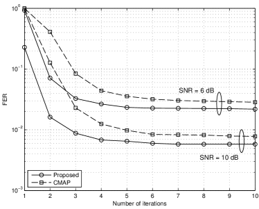
Figure 8: FER of the proposed and CMAP algorithms with respect to the number of iterations performed. The SIR is -4 dB.

In Fig. 8, the FER is shown with respect to the number of iterations where we observe that the proposed algorithm converges 1-2 iterations faster than CMAP. Thus, for $|\mathcal{A}|=L-1$, the proposed algorithm reduces computational complexity by 20–40% due to faster convergence.

VII Conclusion

In this paper, an algorithm is developed which approximates joint MAP detection and equalization in co-channel interference. The approximate MAP algorithm is based on a fully connected factor graph of the joint probability distribution. The algorithm was shown to operate within 0.5 dB of the joint MAP state-space model receiver where the degradation in performance was due to the associated factor graph model. Additionally, the proposed algorithm both improves performance and reduces complexity when compared to the state-of-the-art.

References

- [1] X. Wang and H. Poor, “Iterative (turbo) soft interference cancellation and decoding for coded CDMA,” IEEE Trans. Commun., vol. 47, pp. 1046–1061, Jul. 1999.
- [2] J. Boutros and G. Caire, “Iterative multiuser joint decoding: unified framework and asymptotic analysis,” IEEE Trans. Inf. Theory, vol. 48, pp. 1772–1793, Jul. 2002.
- [3] B. Hochwald and S. ten Brink, “Achieving near-capacity on a multiple-antenna channel,” IEEE Trans. Commun., vol. 51, pp. 389–399, Mar. 2003.
- [4] S. Haykin, M. Sellathurai, Y. de Jong, and T. Willink, “Turbo-MIMO for wireless communications,” IEEE Commun. Mag., vol. 42, pp. 48–53, Oct. 2004.
- [5] R. Visoz and A. Berthet, “Iterative decoding and channel estimation for space-time BICM over MIMO block fading multipath AWGN channel,” IEEE Trans. Commun., vol. 51, pp. 1358–1367, Aug. 2003.
- [6] J. Lee, H. Kwon, and I. Kang, “Interference mitigation in MIMO interference channel via successive single-user soft decoding,” in Proc. Inform. Theory Appl. (ITA) Workshop, 2012, pp. 180–185.
- [7] P. Hammarberg, F. Rusek, and O. Edfors, “Iterative receivers with channel estimation for multi-user MIMO-OFDM: complexity and performance,” EURASIP J. on Wireless Commun. and Netw., vol. 2012, pp. 1–17, Mar. 2012.
- [8] H. Arslan and K. Molnar, “Cochannel interference suppression with successive cancellation in narrow-band systems,” IEEE Commun. Lett., vol. 5, no. 2, pp. 37–39, Feb. 2001.
- [9] J. Andrews, “Interference cancellation for cellular systems: a contemporary overview,” IEEE Wireless Commun. Mag., vol. 12, no. 2, pp. 19–29, Apr. 2005.
- [10] E. Biglieri, R. Calderbank et al., MIMO Wireless Communications. Cambridge University Press, 2007.
- [11] H. Wymeersch, Iterative Receiver Design. Cambridge Univ. Press, 2007.
- [12] T. Moon and J. Gunther, “Multiple-access via turbo joint equalization,” IEEE Trans. Commun., vol. 60, no. 10, pp. 3001–3010, Oct. 2012.
- [13] W. Jiang and D. Li, “Iterative single-antenna interference cancellation: algorithms and results,” IEEE Trans. Veh. Technol., vol. 58, no. 5, pp. 2214–2224, Jun. 2009.
- [14] L. Ping, L. Liu, and W. K. Leung, “A simple approach to near-optimal multiuser detection: interleave-division multiple-access,” in Proc. IEEE Wireless Commun. Netw. Conf., vol. 1, 2003, pp. 391–396.
- [15] F. R. Kschischang, B. J. Frey, and H. A. Loeliger, “Factor graphs and the sum-product algorithm,” IEEE Trans. Inf. Theory, vol. 47, no. 2, pp. 498–519, Feb. 2001.
- [16] L. Bahl, J. Cocke, F. Jelinek, and J. Raviv, “Optimal decoding of linear codes for minimizing symbol error rate (corresp.),” IEEE Trans. Inf. Theory, vol. 20, no. 2, pp. 284–287, Mar. 1974.