Exact sampling of graphs with prescribed degree correlations

Abstract

Many real-world networks exhibit correlations between the node degrees. For instance, in social networks nodes tend to connect to nodes of similar degree and conversely, in biological and technological networks, high-degree nodes tend to be linked with low-degree nodes. Degree correlations also affect the dynamics of processes supported by a network structure, such as the spread of opinions or epidemics. The proper modelling of these systems, i.e., without uncontrolled biases, requires the sampling of networks with a specified set of constraints. We present a solution to the sampling problem when the constraints imposed are the degree correlations. In particular, we develop an exact method to construct and sample graphs with a specified joint-degree matrix, which is a matrix providing the number of edges between all the sets of nodes of a given degree, for all degrees, thus completely specifying all pairwise degree correlations, and additionally, the degree sequence itself. Our algorithm always produces independent samples without backtracking. The complexity of the graph construction algorithm is ${\cal O}(NM)$ where $N$ is the number of nodes and $M$ is the number of edges.

1 Introduction

Complex systems often consist of a discrete set of elements with heterogeneous pairwise interactions. Networks, or graphs have proven to be a useful representational paradigm for the study of these systems [1, 2, 3, 4]. The nodes, or vertices, of the graphs represent the discrete elements, and the edges, or links, represent their interaction. In empirical studies of real-world systems, however, for reasons of methodology, privacy, or simply lack of data, frequently there is only limited information available about the connectivity structure of a network. When this is the case, one has to take a statistical approach and study ensembles of graphs that conform to some structural constraints. This statistical approach enables the computation of ensemble averages of network observables as determined solely by the constraints, i.e., by the specified structural properties of the graphs. Ensemble modeling of this type is necessary to determine the relationship between the given structural constraints and the behavior of the complex system as a whole. Calculating ensemble averages, though, requires the ability to construct all the graphs that are consistent with the required structural constraints, a highly non-trivial problem.

Perhaps one of the simplest examples of structural constraints that occur in data-driven studies of real-world systems is to fix the degree of each node, which is the number of edges that are connected to, or are incident on the node. For an undirected graph with $N$ nodes this information is specified by a degree sequence ${\mathcal{D}}=\left\{d_{1},d_{2},\cdots,d_{N}\right\}$, where $d_{i}$ is the degree of node $i$. Similarly, for a directed graph, a bi-degree sequence (BDS) ${\mathcal{D}}=\left\{\left(d_{1}^{-},d_{1}^{+}\right),\left(d_{2}^{-},d_{2}^{+}\right),\cdots,\left(d_{N}^{-},d_{N}^{+}\right)\right\}$ specifies the number of incoming and outgoing edges for each node where $d_{i}^{-}$ denotes the in-degree, and $d_{i}^{+}$ the out-degree, of node $i$. The situation of most practical interest is when we demand the graph with a given degree sequence to be a simple graph, which has the additional constraints that there can be at most one link (in each direction, if directed) between any two nodes, and that no link starts and ends on the same node (no self-loops). However, not all positive integer sequences can serve as the sequence of the degrees of some simple graph. If such a graph does exist, then the sequence is said to be graphical. Any simple graph (just “graph” from here on) with the prescribed node degrees is said to realize the degree sequence, and it is called a graphical realization of the sequence. The two main results used to test the graphicality of an undirected degree sequence are the Erdős-Gallai theorem [5] and the Havel-Hakimi theorem [6, 7]. For directed networks, instead, the main theorem characterizing the graphicality of a BDS is due to Fulkerson [8]. More recently, exploiting a formulation based on recurrence relations, new methods were introduced to implement these tests with a worst case computational complexity that is only linear in the number of nodes [9, 10, 11]. The advantage of these methods over others with similar complexity [12] is that they also allow a straightforward algorithmic implementation.

While the above results provide complete and practical answers to the question of the graphicality of sequences of integers, they do not suffice to solve the problem of constructing graphs with prescribed degrees. One of the main issues with constructing graphs for the purpose of ensemble modeling is that, except for networks of just a few nodes, the number of graphs realizing a degree sequence, or other possible constraints, is generally so large that their complete enumeration is impractical. Therefore, one has to resort to sampling the space of realizations by randomly generating networks with prescribed node degrees [9, 11]. For the case of degree-based graph sampling, the existing approaches generally fall into two classes that can broadly be referred to as “rewiring” and “stub-matching”. Rewiring methods start from a graph with the required degrees and use Markov chain Monte Carlo (MCMC) schemes to swap repeatedly the ends of pairs of edges to produce new graphs with the same degree sequence [13, 14, 15, 16]. Stub-matching methods, instead, are direct construction algorithms that build the graphs by sequentially creating the edges via the joining of two stubs of two nodes [17, 18, 19, 20, 21]. A stub represents a non-connected, “dangling half-edge” and a node has as many stubs as its degree. Unfortunately, these techniques can provide biased results, or are ill-controlled. In the case of the MCMC method the mixing time is in general unknown and thus one cannot know a priori the number of swaps needed to produce two statistically independent samples. Proofs showing polynomial mixing of the MCMC method have been recently developed for special degree sequences  [22, 23, 24, 25], and for the case of balanced realizations of joint-degree matrices [26]. However, none of these methods allows the determination of the exponent of the polynomial scaling.

Among the stub-matching methods, the most commonly used algorithm, which is also ill controlled, is known as the configuration model. The configuration model was proposed in [17] as an algorithmic equivalent of the results from Refs. [27, 28], themselves based on prior models [29, 30]. The algorithm randomly extracts two stubs from the set of all stubs not yet connected into edges, and connects them into an edge. If a multi-edge or a self-loop has just been created, the process is restarted from the very beginning to avoid biases. However, depending on the degree sequence, this process can become very inefficient with an uncontrolled running time, just like the MCMC method. Alternatively, one can ignore multi-edges and self-loops, and fix them “by hand” at the end of the process. However, doing so produces significant biases even in the limit of large system size [31]. Recently, a novel family of stub-matching algorithms were introduced for both undirected [9] and directed [11] degree sequences (reproduced here in A), based on the so-called star-constrained graphicality theorems [32, 33]. These algorithms generate statistically independent samples with a worst case polynomial time of $O(NM)$, where $M$ is the total number of edges. The samples are not generated uniformly. However, their statistical weights are computable and can be used to obtain results in an importance sampling framework [9, 34, 11, 35]. Note that the solution for the directed sequences also solves the problem for bipartite sequences because a bipartite graph can always be represented as a directed one in which one of the two sets of nodes has only outgoing edges, and the other set has only incoming ones.

Graph construction and sampling becomes even more difficult when there are structural constraints of higher order, such as correlations amongst the node degrees. Degree correlations can be expressed in several ways, for example with the help of the conditional probability $P(d^{\prime}|d)$ that a node of degree $d$ will have a neighbor of degree $d^{\prime}$, or more simply, by the average degree of the neighbors of a node with degree $d$, $\bar{d^{\prime}}(d)=\sum_{d^{\prime}}d^{\prime}P(d^{\prime}|d)$ [36]. The properties of $\bar{d^{\prime}}(d)$ characterize the so-called assortativity of a graph, which is a measure of the tendency of a node to connect to nodes of similar degree. If $\bar{d^{\prime}}(d)$ is increasing in $d$, the graph is degree assortative, if it is decreasing the graph is degree disassortative, and if it is constant, the graph is degree uncorrelated. Even more coarse-grained measures of degree correlations are possible, including the Pearson coefficient [37], the Spearman coefficient [38] and the Kendall coefficient [39]. These coefficients assume values ranging from $-1$, for highly disassortative graphs, to 1, for highly assortative ones.

A more precise way to express degree correlations is via the use of a joint-degree matrix. The joint-degree matrix (JDM) of a given undirected simple graph is a symmetric matrix whose $\left(\alpha,\beta\right)$ element is the number of edges between nodes of degree $\alpha$ and nodes of degree $\beta$. The dimensions of the JDM are $\Delta\times\Delta$, where $\Delta$ is the largest degree of a node in the graph. The degree correlation measures discussed above specify the correlations only statistically, but they do not fix the number of edges between nodes of given degrees, whereas the joint-degree matrices do. In this sense, the relationship between joint-degree matrices and the statistical degree correlation measures is similar to the relationship between degree sequences and degree distributions.

Degree correlations have generated considerable interest, as they are known to affect many structural and dynamical properties of graphs and the processes they support [40, 41, 42, 43, 44, 45, 46, 47]. Nevertheless, even though their importance is well established, it has heretofore not been possible to perform ensemble modeling of graphs with prescribed joint-degree matrices. In this Article, we solve this problem by developing an algorithm based on the stub-matching method to construct and sample ensembles of graphs with a specified joint-degree matrix.

2 Mathematical foundations

2.1 Graphicality of JDMs

The problem of graphicality for JDMs asks whether a specified symmetric matrix can be the JDM of a simple graph. Our starting point is an Erdős-Gallai-like theorem that gives the requiements for a JDM to be graphical [48, 49, 50].

Before stating the theorem, though, note that a JDM specifies uniquely the degree sequence of the graphs that realize it [48]. Given a JDM $J$, the number of nodes with degree $\alpha$ is

$$\left|V_{\alpha}\right|=\frac{1}{\alpha}\left(J_{\alpha\alpha}+\sum_{\beta=1}^{\Delta}J_{\alpha\beta}\right)\>,$$

where $V_{\alpha}$ is the set of nodes, or degree class, with degree $\alpha$. As a general rule of notation we will use lowercase Greek letters to indicate degree values and lowercase Latin letters for node indices. In the equation above the sum of each row $\alpha$ of $J$ is the number of connections involving nodes of degree $\alpha$ (i.e., all nodes in class $V_{\alpha}$). As each node of degree $\alpha$ has exactly $\alpha$ stubs the total number of nodes of degree $\alpha$ is given by the notal number of stubs from all nodes in class $V_{\alpha}$ divided by $\alpha$. Moreover, each edge between nodes of the same degree involves 2 stubs. Thus, the diagonal elements must be double-counted. Note that multiple JDMs can specify the same degree sequence and thus prescribing a JDM is more constraining than only prescribing a degree sequence. With the definitions above, the necessary and sufficient conditions for a JDM to be graphical can be stated as follows [48, 49, 50]:

Theorem 1 (JDM graphicality).

A symmetric $\Delta\times\Delta$ matrix $J$ with non-negative integer elements is a graphical JDM if and only if:

$$1)\quad\left|V_{\alpha}\right|\mathrm{\ is\ an\ integer\ } \forall 1\leqslant\alpha\leqslant\Delta,$$

$$2)\quad J_{\alpha\alpha}\leqslant{{\left|V_{\alpha}\right|}\choose 2} \forall 1\leqslant\alpha\leqslant\Delta,\;\mbox{and}$$

$$3)\quad J_{\alpha\beta}\leqslant\left|V_{\alpha}\right|\left|V_{\beta}\right| \forall 1\leqslant\alpha,\beta\leqslant\Delta\mathrm{\ and\ }\alpha\neq\beta\>.$$

It is important to observe that any graphical realization of a JDM can be decomposed into the disjoint union of a set of subgraphs $G_{\alpha\beta}$ that are bipartite ($\alpha\neq\beta$) with node sets $V_{\alpha}$ and $V_{\beta}$ and $J_{\alpha\beta}$ edges between them or unipartite ($\alpha=\beta$) with node set $V_{\alpha}$ and $J_{\alpha\alpha}$ edges within that set. We are going to call such representation of a graphical realization a degree class representation.

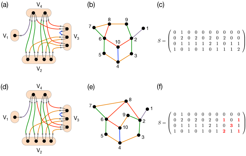
Figure 1: Graphical realizations of a simple JDM, given in (5). Panels (a) and (d) are degree class representations, while panels (b) and (e) are regular representations. The color of the edges indicates the subgraph $G_{\alpha\beta}$ they belong to. Panels (c) and (f) show the corresponding degree-spectra matrices for the two realizations; they differ in the bold red entries.

A simple example of a graphical JDM with $N=10$ and $\Delta=4$ is given by the matrix:

$$J=\left(\begin{array}[]{cccc}0&0&0&1\\ 0&0&4&4\\ 0&4&1&3\\ 1&4&3&0\end{array}\right)\;.$$ (5)

Panels (a) and (b) of Fig. 1 show a graphical realization of $J$ in degree class representation and regular representation, respectively. Panels (d) and (e) of the same figure show another realization of $J$ in the two representations. The color of the edges indicate the subgraph they belong to. For example, $G_{24}$ is a bipartite graph between nodes of degree 2 ($V_{2}$) and 4 ($V_{4}$), respectively, having $J_{2,4}=4$ edges drawn in green color, whereas $G_{33}$ is unipartite with a single $J_{33}=1$ edge drawn in blue. Note that while both graphical realizations have the same JDM, they are very different graphs. To see this, consider the counts $n_{\ell}$ of cycles $C_{\ell}$ of length $\ell$ (a cycle is a closed path without repeated nodes). The graph in Fig. 1(b) has $n_{3}=1$, $n_{4}=2$, $n_{5}=1$, $n_{6}=2$, $n_{7}=3$ and $n_{8}=3$, whereas the one in Fig. 1(e) has $n_{3}=1$, $n_{4}=1$, $n_{5}=2$, $n_{6}=3$, $n_{7}=4$ and $n_{8}=1$.

Theorem 1 is an existence theorem, just like the Erdős-Gallai theorem for the case of degree sequences, and as such it does not provide an algorithm that can generate simple graphs with a given JDM. More importantly, we also need an algorithm that does not exclude classes of graphical realizations of a given JDM, but that can construct in principle any such realization. The situation is similar to that of degree sequences. In that case the Havel-Hakimi method [6, 7] is always able to create a graphical realization of a graphical degree sequence, but cannot construct them all, i.e., there will be some realizations that can never be built by this algorithm. This was the reason for the introduction of the notion of star-constrained graphicality in Refs. [32, 33] and the subsequent construction algorithms in Refs. [9, 11]. Here as well, we want to have a direct construction algorithm and ultimately an exact sampler that does not exclude any realization of a JDM. Due to the different nature of the constraints from the degree-sequence-based case, we need to develop a novel approach.

The idea of the approach is based on the degree class representation above. Since the edges of the subgraphs $G_{\alpha\beta}$ are disjoint, we could build a graphical realization $G$ of the JDM $J$ by building all these subgraphs, while respecting the constraints. For a $G_{\alpha\beta}$ subgraph we know its node set(s) and its total number of edges $J_{\alpha\beta}$. Consider then a node $v\in V_{\alpha}$. We are not given its degree in $G_{\alpha\beta}$ for any $\beta$, but we know that the sum of its degrees within every one of these subgraphs must add up to $\alpha$. For example, the sum of the numbers of the purple, green and red edges coming out of node 2 in Fig. 1(b) must add to 4. In addition, we also have the constraints that the sum of the degrees of one color of all nodes within $V_{\alpha}$ must equal to the corresponding given JDM entry. Indeed, for example, the sum of all green edges in Fig. 1(a) or Fig. 1(b) is $J_{2,4}=4$, for orange is 4, red is 3, etc. Thus, the idea of the algorithm is to first determine the degree of a given color respecting the constraints for all nodes and all colors, then use our methods introduced earlier [9, 11] (see A) to build the $G_{\alpha\beta}$ subgraphs based on the corresponding degree sequences of their nodes. Different graphical realizations will be obtained from different assignments of color degrees and, of course, from the different graphical realizations of the same set of degrees. Note that for the bipartite subgraphs $G_{\alpha\beta}$ we are specifying degree sequences for nodes in both partitions $V_{\alpha}$ and $V_{\beta}$ and thus we can use our graph construction method for directed graphs [11], because a bipartite graph can be represented as a directed graph if nodes in one partition have only outgoing edges and in the other only incoming edges. In the following it will be useful to introduce the notion of degree spectra, representing the degrees of different colors of a node, as described above.

2.2 Degree spectra

Consider a single row $\alpha$ of a graphical JDM $J$. The information contained in the row determines the precise number of edges needed between nodes of degree $\alpha$ and nodes of every degree. In other words, of all the stubs coming from $V_{\alpha}$, $J_{\alpha,1}$ of them must end in a node of degree 1, $J_{\alpha,2}$ of them must end in a node of degree 2, and so on. However, these matrix elements do not specify how to distribute these edges within and between the degree classes. To better specify these connections one introduces the notion of the degree spectra, which can be conveniently represented as a matrix. The degree spectrum of a node is the sequence of its degrees towards all the degree classes, including its own degree class. A degree-spectra matrix $S$ is a $\Delta\times N$ matrix whose $\left(\alpha,i\right)$ element $S_{\alpha i}$ is the number of edges between node $i$ and degree class $\alpha$ (the set of nodes of degree $\alpha$). The $i^{\mathrm{th}}$ column of $S$ defines the degree spectrum of node $i$. Panels (c) and (f) of Fig. 1show two representations of the same JDM given in Eq. 5. In general, there are many degree spectra matrices that correspond to the same JDM. As described in the previous section, we employ a two-step process in order to randomly sample graphs that realize a given JDM. First, we generate a random degree-spectra matrix from the JDM. Second, we construct a random graph that realizes the JDM and that obeys or is consistent with the chosen spectra matrix. This approach creates the need for a method to guarantee that the spectra generated from a JDM are graphical.

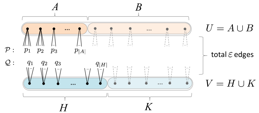
Figure 2: Schematic for the partial degree sequence problem.

The generation of a graphical degree-spectra matrix proceeds systematically, node by node. Therefore, at each step, some nodes will have an already fixed number of links within some of the subgraphs (links of a given color), while for the rest these numbers will not have been determined yet. Thus, at any time during this process we have a partial degree sequence of a bipartite graph. As the subgraphs must be simple graphs (realizable), one must be able to decide whether a partial bipartite degree sequence is graphical. The sufficient and necessary criterion for the graphicality of a partial bipartite degree sequence will be given in Theorem 2 below. However, that will not necessarily mean that the whole JDM $J$ is still realizable, in other words, how do we know that by guaranteeing the graphicality for a subgraph $G_{\alpha\beta}$ we have not precluded graphicality of some other subgraph $G_{\gamma\delta}$, and ultimately of $J$? The answer to this question will be given by Theorem 3, later on. Together, these theorems form the basis for our algorithm to generate graphical degree spectra.

Before proving a theorem that provides a graphicality test for partial bipartite degree sequences, we need to set some notations. Let $A$, $B$, $H$ and $K$ be four sets of nodes:

$$A=\left\{a_{1},a_{2},\cdots,a_{\left|A\right|}\right\} \ \ B=\left\{b_{1},b_{2},\cdots,b_{\left|B\right|}\right\} \quad\mathrm{with\ }A\cap B=\emptyset$$

$$H=\left\{h_{1},h_{2},\cdots,h_{\left|H\right|}\right\} \ \ K=\left\{k_{1},k_{2},\cdots,k_{\left|K\right|}\right\} \quad\mathrm{with\ }H\cap K=\emptyset$$

and let $U=A\cup B$ and $V=H\cup K$ (see Fig. 2). The sets can be of different size, but neither $U$ nor $V$ can be empty. Now, let $\mathcal{P}=\left\{p_{1},p_{2},\cdots,p_{\left|A\right|}\right\}$ and $\mathcal{Q}=\left\{q_{1},q_{2},\cdots,q_{\left|H\right|}\right\}$ be two given sequences of integers. They will represent the partial bipartite degree sequences that have already been fixed by the algorithm up to that point. The degrees of the other nodes, specifically those in the sets $B$ and $K$, are not yet specified. What is specified is the total number of edges $\varepsilon$ in the bipartition, i.e., the total number edges running between the sets $U$ and $V$. Then, the partial bipartite degree sequence triplet $\left(\mathcal{P},\mathcal{Q},\varepsilon\right)$, hereafter simply called a triplet, is graphical if there exists a bipartite graph on $U$ and $V$ with $\varepsilon$ edges and degree sequences $\mathcal{D}(U)\big{|}_{A}=\mathcal{P}$ and $\mathcal{D}(V)\big{|}_{H}=\mathcal{Q}$. In other words, the bipartite graph must be such that the nodes in $A$ have degree sequence $\mathcal{P}$ and those in $H$ have degree sequence $\mathcal{Q}$. The partial degree sequence problem is to decide whether one can choose the degrees of the nodes in the sets $B$ and $K$ such that the above constraints are satisfied and the bipartite degree sequence $\cal D$ is graphical.

Since the graph realizing a triplet is bipartite, the number of edges $\varepsilon$ equals the number of stubs in either set of nodes:

$$\varepsilon=\sum_{i=1}^{\left|U\right|}d_{u_{i}}=\sum_{i=1}^{\left|V\right|}d_{v_{i}}\>.$$

The imposed partial sequences $\mathcal{P}$ and $\mathcal{Q}$ prescribe a certain number of stubs in the first $\left|A\right|$ nodes of $U$ and in the first $\left|H\right|$ nodes of $V$. Let these be $P=\sum_{i=1}^{\left|A\right|}p_{i}$ and $Q=\sum_{i=1}^{\left|H\right|}q_{i}$, respectively. Then, the set $B$ must contain exactly $\varepsilon-P$ stubs; similarly, the set $K$ must contain exactly $\varepsilon-Q$ stubs. With these considerations, we first define the concept of a balanced realization of a triplet. Let $\mu\equiv\frac{\varepsilon-P}{\left|B\right|}$ and $\nu\equiv\frac{\varepsilon-Q}{\left|K\right|}$. A realization of a triplet is defined to be balanced if and only if the degree of any node in $B$ is either $\left\lfloor\mu\right\rfloor$ or $\left\lceil\mu\right\rceil$, and the degree of any node in $K$ is either $\left\lfloor\nu\right\rfloor$ or $\left\lceil\nu\right\rceil$. Notice that this means that if $\mu$ or $\nu$ are integers, then all the nodes in $B$ or $K$ must have exactly degree $\mu$ or $\nu$, respectively. Conversely, if they are not integers, then the degrees of any two nodes in $B$ or in $K$, respectively, can differ at most by 1. That is, a realization is balanced if and only if all the degrees of the nodes that one is free to choose (those in $B$ and $K$) are as close as possible to their averages $\mu$ and $\nu$. The definition can be equivalently formalized by introducing a functional $f$ acting on $B$ and $K$:

$$f\left(B\right) \equiv\sum_{i=1}^{\left|B\right|}\left\lfloor\left|d_{b_{i}}-\mu\right|\right\rfloor\;\;\;\mbox{and}\;\;\;f\left(K\right) \equiv\sum_{i=1}^{\left|K\right|}\left\lfloor\left|d_{k_{i}}-\nu\right|\right\rfloor\>.$$

Then, a realization of a triplet is balanced if and only if both $f\left(B\right)$ and $f\left(K\right)$ vanish.

An important theorem about the graphicality of triplets can now be proven.

Theorem 2.

The triplet $\left(\mathcal{P},\mathcal{Q},\varepsilon\right)$ is graphical if and only if it admits a balanced realization.

Proof.

Sufficiency is obvious. If the triplet admits any realization, balanced or not, it is graphical by definition.

To prove necessity, suppose the triplet is graphical. Then, it admits a realization $G$. If $G$ is balanced, then there is nothing to do. Conversely, if $G$ is not balanced, then $f\left(B\right)$, $f\left(K\right)$, or both, are greater than 0. Without loss of generality, assume that $f\left(B\right)>0$. Then, there exists a node $b_{i}\in B$ such that either $d_{b_{i}}<\left\lfloor\mu\right\rfloor$ or $d_{b_{i}}>\left\lceil\mu\right\rceil$. Again without loss of generality, assume that $d_{b_{i}}<\left\lfloor\mu\right\rfloor$ (the other cases are treated analogously). Then, since the number of stubs within $B$ is fixed, there must exist a node $b_{j}\in B$ such that $d_{b_{j}}>\left\lfloor\mu\right\rfloor$ and thus $d_{b_{j}}>d_{b_{i}}$. But then, there must exist a node $v_{k}\in V$ such that $v_{k}$ is connected to $b_{j}$ but not to $b_{i}$. Now, remove the edge $(v_{k},b_{j})$ and replace it with $(v_{k},b_{i})$. This yields a different realization with the same degrees for the nodes in $V$, and in which $f\left(B\right)$ is decreased by at least 1, as the degrees of $B$ moved towards the balanced condition. The procedure can be repeated until $f\left(B\right)=0$, resulting in a balanced realization. ∎

A key consequence of this theorem is the following.

Corollary 1.

Let $\left(\mathcal{P},\mathcal{Q},\varepsilon\right)$ be a graphical triplet, and let $x$ be a node in $B$ or in $K$. If there is a realization of the triplet in which $d_{x}=\alpha$ and another in which $d_{x}=\beta$, with $\alpha<\beta$, then for all $\gamma$ with $\alpha\leqslant\gamma\leqslant\beta$ there exists a realization in which $d_{x}=\gamma$.

Proof.

Without loss of generality, assume $x\in B$. Then, there are several cases, each determined by the relative values of $\alpha$, $\beta$ and $\left\lfloor\mu\right\rfloor$. The most general case is $\alpha<\left\lfloor\mu\right\rfloor<\beta$, so consider only this situation. Start from the realization with $d_{x}=\beta$. Repeated applications of the method in the proof of Theorem 2 will eventually yield a realization in which $d_{x}=\left\lfloor\mu\right\rfloor$. For each step, the degree of $x$ will have decreased by 1. Therefore, one realization of the triplet will have been found with $d_{x}=\gamma$ for all $\left\lfloor\mu\right\rfloor\leqslant\gamma\leqslant\beta$.

Now, start from the realization with $d_{x}=\alpha$. Applying the same step from the proof of Theorem 2 repeatedly will eventually yield a realization in which $d_{x}=\left\lfloor\mu\right\rfloor$. For each of these steps, the degree of $x$ will have increased by 1. Therefore, one realization of the triplet will have been found with $d_{x}=\alpha$ for all $\alpha\leqslant\gamma\leqslant\left\lfloor\mu\right\rfloor$. ∎

Notice that, given a graphical triplet, Corollary 1 also implies the existence of minimum and maximum allowed degrees for each node whose degree has not yet been fixed in that triplet (namely, in $B$ and $K$). That is, a realization of the triplet exists with a node having either its minimum or maximum degree, or any degree between these two values. Of course, the value of the minimum and maximum degree will depend on which degrees have been fixed up to that point, so these need to be computed on the fly. How to calculate these degree bounds will be explained in Subsection 3.1.

2.3 Building a degree-spectra matrix

Corollary 1 suggests the possibility of a direct, sequential way to build a degree-spectra matrix from a JDM. However, building the degree-spectra matrix node by node is a local process, which guarantees via Theorem 2 only that the bipartite graph in which the node whose degree spectrum is being set resides is graphical. There is a global constraint, however, on every node, namely that the sum of their degree spectra must add up to the degree of the class they belong to. We have to make sure that the local construction process also respects the global constraints, i.e., it is feasible with it. The theorem below will show that this sequential construction process is feasible, and just as importantly, all graphical realizations of a JDM $J$ can be constructed in this way, i.e., all graphical degree-spectra matrices can be obtained by this sequential construction process.

Theorem 3.

Let ${\cal S}$ be the subset of all the nodes with fixed spectra; then, there exists a realization of a JDM $J$ consistent with the fixed spectra if and only if for every $(\alpha,\beta)$ pair with $\alpha,\beta\in\{1,\ldots,\Delta\}$ there exists a graph $G_{\alpha\beta}$ with $J_{\alpha,\beta}$ edges also satisfying the fixed spectra of ${\cal S}$.

Proof.

Necessity is obvious. If there exists a realization of $J$ satisfying the spectra, then each subgraph between any pair of degree classes both satisfies the spectra and has the right number of edges.

To prove sufficiency, assume that we have a fixed degree spectrum for all the nodes in ${\cal S}$ and we have guaranteed the graphicality of all the subgraphs $G_{\alpha\beta}$. They have the right number of edges $J_{\alpha,\beta}$ and their nodes satisfy the fixed spectra specified in the subset ${\cal S}$. Since we have guaranteed graphicality for all the $G_{\alpha\beta}$ subgraphs with these constraints, let us consider some graphical realization for each such subgraph and consider their union graph $G$. If the “free” nodes, i.e., those without a fixed spectrum, have all the correct degree in $G$ (i.e., every node $v\in V_{\alpha}$ has $d_{v}=\alpha$ for all $\alpha$), then there is nothing to do. Now, assume they don’t. Since the total number of edges in each $G_{\alpha\beta}$ is correct by hypothesis, there must exist a degree $\alpha$ and two free nodes $v$ and $w$ belonging to $V_{\alpha}$ such that $d_{v}<\alpha$ and $d_{w}>\alpha$. Thus, there must exist a node $u$ connected to $w$ but not to $v$. Then, erase the edge $(u,w)$, and replace it with $(u,v)$. This leaves the numbers of edges in all $G_{\alpha\beta}$ unchanged, and does not change the degree spectrum of $u$, because $v$ and $w$ belong to the same degree class. Repeating this procedure results eventually in all the nodes having the correct degree. ∎

Theorem 3 is fundamentally important as it justifies a systematic, node-by-node approach in building a graphical degree-spectra matrix. In fact, so long as one guarantees the possibility of subgraphs with the correct number of edges, a partial degree-spectra matrix maintains the graphicality of the JDM.

The only detail left is specifying how to choose the numbers that form the degree spectra. Fortunately, this is straightforward. As mentioned in the previous Subsection, an implication of Corollary 1 is the existence of minimum and maximum allowed degrees for nodes in partial degree sequences. Let them be $m$ (minimum) and $M$ (maximum). But a partial degree sequence is nothing else than a partially built degree spectrum, if one recognizes the node sets $U$ and $V$ as two degree classes. Then, a condition that must be satisfied in building a degree-spectra matrix is that any new number chosen to augment a partially built degree spectrum has to be within these bounds. However, one must also consider that if a node belongs to a certain degree class, it must have the correct total degree.

To state both conditions, assume the degree spectrum of node $v\in V_{\alpha}$ is being built. Let $\Gamma$ be the set of degree classes for which a spectrum element has already been chosen, and let $S_{\beta v}$ be the element to determine next. Then, a valid value $k$ for $S_{\beta v}$ must satisfy the two conditions

$$m_{\beta}\leqslant k\leqslant M_{\beta}$$ (6)

$$\sum_{\eta\notin\left(\Gamma\cup\beta\right)}m_{\eta}\leqslant\alpha-k-\sum_{\eta\in\Gamma}S_{\eta v}\leqslant\sum_{\eta\notin\left(\Gamma\cup\beta\right)}M_{\eta}\>.$$ (7)

Below, in Subsection 3.1 we describe how to compute the min and max values for degree spectra elements.

3 The algorithm

3.1 Description

We are now ready to describe our JDM sampling algorithm. The algorithm is composed of two parts. The first is a spectra sampler that randomly generates degree-spectra matrices from a graphical JDM $J$:

1. Initialize $i=1$.

2. Set $\alpha=1$.

3. Let $l$ be the number of the residual, unallocated stubs of node $i$. If $l≠0$:

   1. If $J_{d_{i},\alpha}≠0$:

      1. For all $\alpha\leqslant\beta\leqslant\Delta$, if $J_{d_{i},\beta}≠0$, find $M_{k}$ and $m_{k}$; otherwise, set $m_{k}=M_{k}=0$.

      2. Compute $t=\sum_{\beta=\alpha+1}^{\Delta}m_{\beta}$ and $T=\sum_{\beta=\alpha+1}^{\Delta}M_{\beta}$.

      3. Find the actual minimum and maximum allowed for the degree-spectrum element: $r=\max\left\{m_{\alpha},l-T\right\}$ and $R=\min\left\{M_{\alpha},l-t\right\}$.

      4. Extract an integer $S_{\alpha,i}$ uniformly at random between $r$ and $R$.

   2. Increase $\alpha$ by 1, and go to step (iii).

4. Increase $i$ by 1. If $i\leqslant N$, go to step (ii).

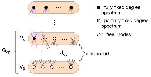
Figure 3: Sequentially determining graphical degree spectra consistent with a given JDM $J$.

To find the values of $m$ and $M$ in step (iii).a.1 above, consider the degrees of the nodes belonging to $V_{\alpha}$ and $V_{\beta}$ in $G_{\alpha\beta}$. In the formalism of Subsection 2.2, the already fixed spectra elements are equivalent to the sequences $\mathcal{P}$ and $\mathcal{Q}$. Then, to test the viability of a given value as a degree-spectrum element, assign it to the element being determined, complete the degree sequence making it balanced, and test it for graphicality, see Fig. 3. If the sequence is graphical, then the triplet has a balanced realization, which by Theorem 2 is a necessary and sufficient condition for the existence of a subgraph corresponding to the spectrum element being determined. If $G_{\alpha\beta}$ is unipartite, the graphicality test can be done using the fast method described in [9]. The situation is marginally different if $G_{\alpha\beta}$ is bipartite. In this case, as previously mentioned, the degree sequence can be built as a BDS in which nodes of degree $\alpha$ only have incoming edges, and nodes of degree $\beta$ only have outgoing ones. This sequence can then be tested with the fast directed graphicality test described in [11].

Thus, to find the minimum value $m$ one can simply run a sequential test, checking for valid spectrum values from 0 onwards. The first successful value is $m$. Then, to find $M$, use bisection to test all the values from $m+1$ to the theoretical maximum, looking for the largest number allowed. Clearly, the theoretical maximum at that stage is the degree of the class the node belongs to minus the sum of the already fixed spectra values for that degree.

These considerations also clarify the nature of the second part of the algorithm, which samples realizations of the JDM from an extracted degree spectra matrix. Summarizing,

• JDM realizations can be decomposed into a set of independent unipartite and bipartite graphs.

• The degree spectra define the degree sequences of the component subgraphs.

Then, to accomplish the actual sampling, extract the degree sequences from the degree spectra and use them in the graph sampling algorithms for undirected and directed graphs presented in [9, 11] and in here in A. Every time a sample is generated, it constitutes a subgraph of a JDM realization. All that is needed in the end is simply to list the edges correctly, since the graph realizing the JDM is the union of all the unipartite and bipartite subgraphs into which it has been decomposed.

3.2 Sampling weights

Our algorithm does not extract all degree-spectra matrices from a JDM with the same probability. However, the relative probability for the extraction of each spectra matrix is easily computed, and it can be used to reweight the sample and obtain unbiased sampling. If every new element of a degree-spectra matrix is extracted uniformly at random between $r$ and $R$, its probability of being chosen is simply $\frac{1}{R-r+1}$. Therefore, the probability of extracting a given spectra matrix $S$ is $p\left(S\right)=\prod_{i=1}^{m}\frac{1}{R-r+1}$, where $m$ is the total number of elements extracted. Then, an unbiased estimator for a network observable $Q$ on an ensemble of $Z$ spectra matrices can be computed using the weighted average

$$\left\langle Q\right\rangle=\frac{\sum_{i=1}^{Z}Q_{i}w_{i}}{\sum_{i=1}^{Z}w_{i}}\>.$$ (8)

In the expression above, $Q_{i}$ is the value that $Q$ assumes on the $i^{\mathrm{th}}$ sampled matrix. Indicating by $r_{j}$ and $R_{j}$ the values that $r$ and $R$ assume for the $j^{\mathrm{th}}$ matrix element extracted, the weights are

$$w_{i}=\prod_{j=1}^{m}\left(R_{j}-r_{j}+1\right)\>.$$ (9)

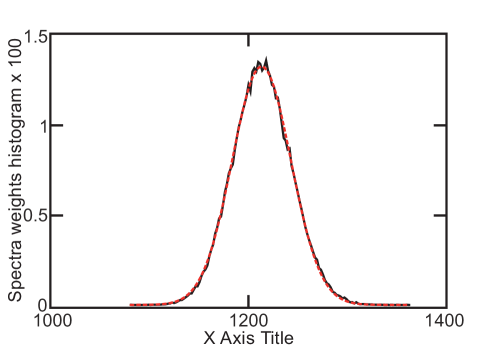
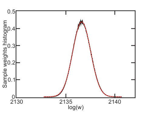
Figure 4: Log-normal distribution of weights. The top panel shows the histogram of the natural logarithms of the weights for an ensemble of $10^{5}$ degree-spectra matrices; the bottom panel shows the histogram for an ensemble of $10^{8}$ sample weights. Both distributions (solid black lines) are well fitted by a Gaussian curve (dashed red line).

Of course, besides the spectra matrix, every subgraph has its own sampling weight. Thus, the total weight of a single JDM sample is the product of the corresponding spectrum weight and all the subgraph weights. To describe the distribution of the sample weights, first recall that the individual subgraph weights are log-normally distributed [9, 11]. Thus, as the sample weights are their product, we expect them to be log-normally distributed too. Also, for large JDMs, where $\Delta^{2}\gg 1$, the $m$ factors in Eq. 9 are effectively random. Thus, our expectation is that the spectra weights are log-normally distributed as well. To verify this, we extracted the JDM of a random scale-free network with 1000 nodes and power-law exponent of $2.5$, and used it to generate an ensemble of $10^{5}$ degree spectra matrices and one of $10^{8}$ JDM samples of a single spectra matrix. Figure 4 shows that the histograms of the logarithms of spectra matrix weights and sample weights are well approximated by a Gaussian fit, supporting our assumptions.

A simple and small example is provided in B. There, we analytically compute the JDM ensemble averages of the local clustering coefficients of nodes of all degrees, based on unweighted sampling and also based on weighted sampling, with the weights provided by the algorithm. In table 1, we show the results of simulations using our algorithm, taking into account the sample weights (as described above), and simply computing the averages of the clustering coefficients over the samples generated. The results between theoretical and simulated measures agree very well. The differences between weighted and unweighted versions can be also appreciated, and while they are small in this example, they are measurable and need to be taken into account in general.

3.3 Computational complexity

To determine the computational complexity of the algorithm, first note that the main cost in creating a spectra matrix comes from the repeated graphicality tests. Let $A$ be the number of non-empty degree classes in the JDM

$$A=\left|\left\{\alpha:\ V_{\alpha}≠\emptyset\right\}\right|\>.$$

Then, for each of the $NA$ non-trivial elements in the degree-spectra matrix, $A$ tests are needed, each with a computational complexity of the order of the number of nodes in the corresponding degree class. Thus, the total computational complexity for the spectra construction part of the algorithm is

$$C_{S}={\cal O}\left(N\sum_{\alpha=1}^{\Delta}\sum_{\beta=\alpha}^{\Delta}\left|V_{\beta}\right|\right)\>.$$ (10)

Notice that in our treatment one is free to choose the order of the degree classes. Thus, to minimize the complexity, one can simply determine the degree-spectra elements in descending order of degree class size. Then, the worst case corresponds to the equipartition of the nodes amongst degree classes, $\left|V_{\alpha}\right|=\frac{N}{A}$. In this case, it is

$$C_{S}={\cal O}\left(NA^{2}\frac{N}{A}\right)={\cal O}\left(N^{2}A\right)\>,$$

which reduces to

$$C_{S}={\cal O}\left(N^{3}\right)$$

if the number of degree classes is of the same order as the number of nodes.

A more precise estimate for a given JDM can be obtained by rewriting Eq. 10 as

$$C_{S}={\cal O}\left(N^{2}\sum_{\alpha=1}^{\Delta}\sum_{\beta=\alpha}^{\Delta}P\left(\beta\right)\right)\>,$$

where the degree distribution $P\left(d\right)=\left|V_{d}\right|/N$ is the probability that a randomly chosen node has degree $d$. It is easy to see, then, that the worst case is unlikely to occur. Consider for instance systems of widespread insterest, such as scale-free networks, for which $P\left(d\right)\sim d^{-\gamma}$ with $\gamma>2$. Then, in the limit of large networks, the equation above becomes

$$C_{S}={\cal O}\left(N^{2}\int_{1}^{\infty}\mathrm{dx}\int_{x}^{\infty}\mathrm{dk}\left(\gamma-1\right)k^{-\gamma}\right)={\cal O}\left(\frac{N^{2}}{\gamma-2}\right)={\cal O}\left(N^{2}\right)\>.$$

Thus, in this case, the complexity leading order for spectra matrix extraction is only quadratic.

Given a degree-spectra matrix, to construct a JDM realization one then needs to build ${\cal O}\left(A^{2}\right)$ subgraphs, each with ${\cal O}\left(\frac{N}{A}\right)$ nodes and ${\cal O}\left(\frac{M}{A}\right)$ edges. For each subgraph, the computational complexity is of the order of the number of nodes multiplied by the number of edges. Thus, the total sampling complexity is ${\cal O}\left(A^{2}\frac{N}{A}\frac{M}{A}\right)={\cal O}\left(NM\right)$. Therefore, the total complexity of the graph construction part of our method is ${\cal O}\left(N^{2}\right)$ for sparse networks, and ${\cal O}\left(N^{3}\right)$ for dense ones. Once more, we do not expect the worst case complexity to occur often. For example, in the already mentioned case of scale-free networks, which are always sparse [51], the total complexity of our algorithm would only be quadratic. A less efficient sampling method has been developed recently [52], but it is based on backtracking, producing results containing biases that are uncontrolled and that cannot be estimated.

4 Conclusions

In summary, we have solved the problem of constrained graphicality when degree correlations are specified, developing an exact algorithm to construct and sample graphs with a specified joint-degree matrix. A JDM specifies the number of edges that occur between degree classes of nodes (nodes of given degrees), and thus completely determines all pairwise degree correlations in its realizations. Our algorithm is guaranteed to successfully build a random JDM sample in polynomial time, systematically, and without backtracking. It is also guaranteed to be able to build any of the graphical realizations of a JDM. Each graph is constructed independently and thus there are no correlations between samples. Although the algorithm does introduce a sample bias, the relative probability for the construction of each sample is computable, which allows the use of weighted averages to obtain unbiased sampling (importance sampling). However, importance sampling is only exact in the limit of an infinite number of samples. This raises the issue of convergence. The lognormal distribution of weights makes convergence slow, but for small- to medium-sized networks good accuracy can be achieved, and quantities computed as if from uniform sampling. Improving the speed of convergence is a challenging problem, partly because it depends on the constraining JDM, and will be addressed in future publications.

Degree correlations in real-world systems have been widely observed. Social networks are known to be positively correlated, and the concept of assortativity was known to the sociological literature before it was employed in applied mathematics. Technological networks are also characterized by particular correlation profiles. Moreover, correlations significantly affect the dynamics of spatial processes, such as the spread of epidemics [3]. Thus, with our algorithm, one can model correctly complex systems of general interest with desired degree assortativity. For the first time, this enables the study of networks in which the correlations are not determined solely by the nodes’ degrees. For instance, there exist many studies about social networks, consisting of a comparison between some specific real-world network and a randomized ensemble of networks with the same degree sequence or degree distribution. As social networks are scale-free, these studies often just sample the same sequence or the same type of power-law sequences to produce null-model results. However, social networks are assortative, while random scale-free networks are on average disassortative. Thus, the average correlations of scale-free networks make degree-sequence and degree-distribution sampling problematic if one is trying to consider a random model of a social network. Our method allows one to avoid this problem by directly imposing the correlations, rather obtaining only those imposed by the degree sequence.

Upper bounds on the computational complexity of our algorithm show that in the worst case it is cubic in the number of nodes. However, we provide a way to compute the expected worst-case complexity if the degree distribution of the networks considered is known. This shows that, for commonly studied cases such as scale-free networks, the maximum complexity is only of the order of $N^{2}$, making the algorithm even more efficient.

Appendix A Direct construction of random directed and undirected graphs with prescribed degree sequence

In order to fully describe our algorithm for sampling graphs with prescribed degree correlations, we include in this appendix succinct descriptions of our algorithms for sampling random undirected [9] and directed [11] graphs with a prescribed degree sequence. Both are used in our algorithm to sample graphs with a prescribed JDM, and both work by directly constructing the graphs. So long as the prescribed degree sequence is graphical, both algorithms are guaranteed to successfully construct a graph without backtracking. They accomplish this by building the graph an edge at a time, connecting pairs of stubs, maintaining the graphicality of the residual stubs throughout the construction process. The algorithms make use of our fast methods for testing the graphicality of degree sequences, which are also described below. The worst case complexity is ${\mathcal{O}}\left(N\right)$ for the graphicality tests, and ${\mathcal{O}}\left(NM\right)$ for both sampling algorithms. Both algorithms generate biased samples, but we also state the relative probability of generating a sample, which can be used to calculate unbiased statistical averages. See our previous publications for proof of the correctness of these algorithms [9, 11]; they are stated without proof or detailed explanation here.

A.1 Undirected graphs

A nonincreasing sequence of integers ${\mathcal{D}}=\left\{d_{1},d_{1},\dots,d_{N}\right\}$ is graphical if and only if $\sum_{i=1}^{N}d_{i}$ is even, and $L_{k}\leqslant R_{k}$ for all $1\leqslant k<N$, where $L_{k}$ and $R_{k}$ are given by the recurrence relations

$$L_{1} =d_{1}$$ (11)

$$L_{k} =L_{k-1}+d_{k}$$ (12)

and

$$R_{1} =N-1$$ (13)

$$R_{k} =\left\{\begin{array}[]{l}R_{k-1}+x_{k}-2\quad\ \,\forall k<k^{\ast}\\ R_{k-1}+2(k-1)-d_{k}\quad\forall k\geqslant k^{\ast}\end{array}\right.$$ (16)

and we defined the crossing indices $x_{k}=\min\left\{i:d_{i}<k\right\}$, and $k^{\ast}=\min\left\{i:x_{i}<i+1\right\}$. Thus, to test the graphicality of ${\mathcal{D}}$:

1. Sum the degrees to determine if $\sum_{i=1}^{N}d_{i}$ is even. If false, then stop; ${\mathcal{D}}$ is not graphical. If true, continue. While summing the degrees, also calculate the crossing indices $x_{k}$ for each $k$ and determine $k^{*}$.

2. Test if $L_{1}\leq R_{1}=N-1$. If false, then stop; ${\mathcal{D}}$ is not graphical. If true, set $k=2$ and continue.

3. Test if $L_{k}\leq R_{k}$. If false, then stop; ${\mathcal{D}}$ is not graphical. If true, increase $k$ by one and repeat. Continue until $k=N-1$, then stop; ${\mathcal{D}}$ is graphical.

Given a nonincreasing graphical degree sequence ${\mathcal{D}}$, a random undirected graph that realizes ${\mathcal{D}}$ can be constructed by:

1. To each node, assign a number of stubs equal to its degree.

2. Choose a hub node $i$. Any node can in principle be chosen, for example, the node with the largest degree.

3. Create a set of forbidden nodes $X$, which initially contains only $i$.

4. Find the set of allowed nodes $A$ to which $i$ can be linked preserving the graphicality of the remaining construction process. To find $A$, first determine the maximum fail degree $\kappa$ using the method described below. Then $A$ will consist of all nodes $j\notin X$ that have remaining degree greater than $\kappa$.

5. Choose a random node $m\in A$ and connect $i$ to it.

6. Reduce the value of $d_{i}$ and $d_{m}$ in ${\mathcal{D}}$ by 1, and reorder it.

7. If $m$ still has unconnected stubs, add it to the set of forbidden nodes $X$.

8. If $i$ still has unconnected stubs, return to step (iv).

9. If nodes still have unconnected stubs, return to step (ii).

To determine the maximum fail degree in a degree sequence $\mathcal{D}$ being sampled, build the residual degree sequence $\mathcal{D}^{\prime}$, by connecting the hub node $i$ with remaining degree $d_{i}$ to the $d_{i}-1$ nodes with the largest degrees that are not in the forbidden set $X$ and reducing the elements of ${\mathcal{D}}$ accordingly. Then, compute the graphicality test inequalitites. Each inequality potentially yields a fail-degree candidate, depending on the values of $L_{k}$ and $R_{k}$. For each value of $k$ there are only 3 possibilities:

1. $L_{k}=R_{k}$

2. $L_{k}=R_{k}-1$

3. $L_{k}\leqslant R_{k}-2$

In case (a), the degree of the first non-forbidden node whose index is greater than $k$ is the fail-degree candidate. In case (b), the degree of the first non-forbidden node whose index is greater than $k$ and whose degree is less than $k+1$ is the fail-degree candidate. In case (c), there is no fail-degree candidate. The sequence of candidate nodes is non-decreasing until the fail-degree is found. Thus, one can stop the calculation when either the current fail-degree candidate is less than the previous one, or when a case (a) happens.

This algorithm generates graph samples biasedly. However, the relative probability of generating a particular sample $\mu$ is

$$p_{\mu}=\prod_{i=1}^{m}\bar{d}_{i}!\prod_{j=1}^{\bar{d}_{i}}\frac{1}{\left|A_{i_{j}}\right|}\>,$$ (17)

where $\bar{d}_{i}$ is the residual degree of node $i$ when it is chosen as a hub, $m$ is the total number of hubs used, and $A_{i_{j}}$ is the allowed set for the $j^{\mathrm{th}}$ link of hub $i$. Thus, an unbiased estimator for a network observable $Q$ for any target distribution $P$ is the weighted average

$$\left\langle Q\right\rangle=\frac{\sum_{i=1}^{M}Q_{\mu_{i}}w_{\mu_{i}}P\left(\mu_{i}\right)}{\sum_{i=1}^{M}w_{\mu_{i}}P\left(\mu_{i}\right)}\>,$$ (18)

where $M$ is the number of samples and $w_{\mu_{i}}=p_{\mu_{i}}^{-1}$. For uniformly sampling the networks, $P$ is constant and it cancels out of the formula.

A.2 Directed graphs

A bi-degree sequence (BDS) $\mathcal{D}=\left\{\left(d_{1}^{-},d_{1}^{+}\right),\left(d_{2}^{-},d_{2}^{+}\right),\dots,\left(d_{N}^{-},d_{N}^{+}\right)\right\}$ of integer pairs, ordered so that the first elements of each pair form a non-increasing sequence, is graphical if and only if $\sum_{i=1}^{N}d_{i}^{-}=\sum_{i=1}^{N}d_{i}^{+}$, and $L_{k}\leqslant R_{k}$ for all $1\leqslant k\leqslant N-1$, where $L_{k}$ and $R_{k}$ are given by the recurrence relations

$$L_{1} =d_{1}^{-}$$ (19)

$$L_{k} =L_{k-1}+d_{k}$$ (20)

and

$$R_{1} =N-1-G_{1}\left(0\right)$$ (21)

$$R_{k} =\left\{\begin{array}[]{l}R_{k-1}+N-\bar{G}_{k-1}\left(k-1\right)\quad\quad\forall d_{k}^{+}<k\\ R_{k-1}+N-\bar{G}_{k-1}\left(k-1\right)-1\quad\forall d_{k}^{+}\geqslant k\\ \end{array}\right.\>,$$ (24)

and $G_{k}$ and $\bar{G}_{k}$ are defined as follows. Let

$$g_{i}\left(k\right)=\left\{\begin{array}[]{l}d_{i}^{+}+1\quad\forall i\leqslant k\\ d_{i}^{+}\quad\quad\forall i>k\\ \end{array}\right.\>.$$ (25)

Then

$$G_{k}\left(p\right)=\sum_{i=1}^{N}\delta_{p,g_{i}\left(k\right)}\>,$$ (26)

where $\delta$ is the Kronecker delta, and $\bar{G}$ is given by the recurrence relation

$$\bar{G}_{1}\left(1\right) =G_{1}\left(0\right)+G_{1}\left(1\right)$$ (27)

$$\bar{G}_{k}\left(k\right) =\bar{G}_{k-1}\left(k-1\right)+G_{1}\left(k\right)+S\left(k\right)\>,$$ (28)

where

$$S\left(k\right)\equiv\sum_{t=2}^{k-1}\delta_{k,d_{t}^{+}+1}-\sum_{t=2}^{k}\delta_{k,d_{t}^{+}}\>.$$ (29)

To efficiently test the graphicality of a BDS ${\mathcal{D}}$,

1. Sum the in- and out-degrees to determine if $\sum_{i=1}^{N}d_{i}^{-}=\sum_{i=1}^{N}d_{i}^{+}$. If false, then stop; ${\mathcal{D}}$ is not graphical. If true, continue. While summing the degrees, also calculate $L_{k}$ for each $k$.

2. Compute $G_{1}\left(k\right)$ for each $k$.

3. Compute $S\left(k\right)$ for all $k$:

   1. Initialize $S\left(k\right)$ to 0 for all $k$. Set $i=2$.

   2. If $d_{i}^{+}\geqslant i$, decrease $S\left(d_{i}^{+}\right)$ by 1.

   3. If $d_{i}^{+}+1>i$, increase $S\left(d_{i}^{+}+1\right)$ by 1.

   4. Increase $i$ by 1. If $i\leqslant N$, repeat from step (b).

4. Test if $L_{1}\leq R_{1}$. If false, then stop; ${\mathcal{D}}$ is not graphical. If true, set $k=2$ and continue.

5. Test if $L_{k}\leq R_{k}$. If false, then stop; ${\mathcal{D}}$ is not graphical. If true, increase $k$ by one and repeat. Continue until $k=N-1$, then stop; ${\mathcal{D}}$ is graphical.

Given a graphical BDS of integer pairs ${\mathcal{D}}$ in lexicographic order, a random directed graph that realizes ${\mathcal{D}}$ can be constructed by

1. Assign in-stubs and out-stubs to each node according to its degrees.

2. Define as current hub the lowest-index node $i$ with non-zero out-degree.

3. Create a set of forbidden nodes $X$, which initially contains $i$ and all nodes with zero in-degree.

4. Find the set of allowed nodes $A$ to which an out-stub of $i$ can be connected without breaking graphicality. To find $A$, first determine the maximum fail in-degree $\kappa$ using the method described below. Then $A$ will consist of all nodes $j\notin X$ that have remaining in-degree greater than $\kappa$.

5. Choose a random node $m\in A$ and connect an out-stub of $i$ to one of its in-stubs.

6. Reduce the value of $d_{i}^{+}$ and $d_{m}^{-}$ in ${\mathcal{D}}$ by 1, and reorder it accordingly.

7. Add $m$ to the set of forbidden nodes $X$.

8. If $i$ still has unconnected out-stubs remaining, return to step (iv).

9. If nodes still have unconnected out-stubs, return to step (ii).

The following simple procedure can be used to efficiently find the fail-in-degree in step (iv) of the sampling algorithm.

1. Create a new BDS $\mathcal{D}^{\prime}$ obtained from $\mathcal{D}$ by reducing the in-degrees of the first $d_{i}^{+}-1$ non-forbidden nodes by 1, and reducing the out-degree of $i$ to 1.

2. If $i=1$, set $k=2$; otherwise, set $k=1$.

3. Compute ${L_{k}}$ and ${R_{k}}$ of the BDS $\mathcal{D}^{\prime}$.

4. If ${L_{k}}\neq{R_{k}}$: increase $k$ by 1; if $k=N$, there is no fail-in-degree, and all the non-forbidden nodes are allowed, so stop; otherwise, go to step (iii).

5. Find the first non-forbidden node in $\mathcal{D}^{\prime}$ whose index is greater than $k$.

6. Identify this node in the original BDS $\mathcal{D}$. Its in-degree is the fail-in-degree. Stop.

As in the case of the sampling algorithm for undirected graphs, this algorithm generates directed graph samples biasedly. However, an unbiased estimator for a network observable $Q$ for any target distribution $P$ is the weighted average given by Eq. 18. In this case the weights are

$$w_{\mu}=\prod_{i=1}^{\nu}\prod_{j=1}^{d_{i}^{+}}\left|A_{i_{j}}\right|\>,$$ (30)

where $\nu$ is the total number of hubs used, $\left|A_{i_{j}}\right|$ is the size of the allowed set immediately before placing the $j^{\mathrm{th}}$ connection coming from the $i^{\mathrm{th}}$ hub, and $d_{i}^{+}$ is the out-degree of the $i^{\mathrm{th}}$ node chosen as a hub. Note that, unlike the case for undirected networks, there is no factorial combinatorial factor in the weights. This is because while the particular sequence of hub nodes chosen depends on the links placed, every node with non-zero out-degree will be selected, sooner or later, as the hub. Therefore, all the samples produced would have an extra, identical, multiplicative factor of $\prod_{i=1}^{N}\frac{1}{d_{i}^{+}!}$. As only the relative probabilities are needed for estimating an observable, and this factor is the same for every possible sample, it is eliminated from the formula for the weights.

Appendix B An explicit example

To illustrate the sampling mechanism and the difference between weighted and unweighted estimation, we consider the realizations of the JDM

$$J=\left(\begin{array}[]{ccc}0&0&0\\ 0&2&4\\ 0&4&1\\ \end{array}\right)\>,$$ (31)

and explicitly compute the average local clustering coefficients $\left\langle c_{d}\right\rangle$ of the nodes of degree $d$, for all values of $d$. This JDM induces the degree sequence ${\mathcal{D}}=\left\{2,2,2,2,3,3\right\}$, and, up to isomorphism, has only three possible realizations, shown in Fig. 5.

Figure 5: Possible realizations of the JDM in Eq. 31, up to isomorphism.

From the figures, it is easy to see that, for the pentagon graphs, $\left\langle c_{2}\right\rangle_{P}=1/4$ and $\left\langle c_{3}\right\rangle_{P}=1/3$. Also, for the hexagon graphs $\left\langle c_{2}\right\rangle_{H}=\left\langle c_{3}\right\rangle_{H}=0$, while for the bow tie graphs $\left\langle c_{2}\right\rangle_{B}=1$ and $\left\langle c_{3}\right\rangle_{B}=1/3$.

B.1 Unweighted estimate

To calculate the theoretical results for the unweighted case, we need to consider the probability with which our algorithm generates each degree-spectra matrix from $J$. To this purpose, first note that there are several degree-spectra matrices whose realizations are all pentagon graphs. Also, all the hexagon and bow tie graphs have the same degree-spectra matrix

$$S_{HB}=\left(\begin{array}[]{cccccc}0&0&0&0&0&0\\ 1&1&1&1&2&2\\ 1&1&1&1&1&1\\ \end{array}\right)\>.$$ (32)

This allows us to compute just the probability of generating $S$, as all the other matrices will yield the same contribution to $\left\langle c_{2}\right\rangle_{P}$ and $\left\langle c_{3}\right\rangle_{P}$.

Our method chooses the elements of the degree-spectra matrix $S$ being created in a systematic way, node by node. As there are no nodes of degree 1, all the element in the first row of the matrix are fixed to 0. Then, the first element to choose is $S_{2,1}$, that is, the number of edges between node 1 and nodes of degree 2. The possible choices for this element are 0, 1, and 2. Choosing 0 or 2 will result necessarily in a degree-spectra matrix whose realizations are all pentagon graphs. In fact, from Fig. 5 one can see that, amongst the realizations of $J$, the pentagon graphs are the only ones in which a node of degree 2, such as node 1, has either no edges or 2 edges with nodes of degree 2. Thus, choosing the value of $S_{2,1}$ with uniform probability, at this stage one generates pentagon graphs with probability $2/3$.

The remaining choice, $S_{2,1}=1$, happens with probability $1/3$. In this case, $S_{3,1}$ is forced to be 1, since the elements in the first column of $S$ must sum up to the degree of the node 1, which is 2. The next element to determine is then $S_{2_{2}}$. Similarly to the previous case, the possible values are 0, 1, and 2. Choosing 0 or 2 will always result in pentagon graphs, whose probability of being generated increases by $1/3\cdot 2/3=2/9$.

Choosing $S_{2,2}=1$, which occurs with total probability $1/3\cdot 1/3=1/9$, forces $S_{3,2}=1$. The next value to determine is that of $S_{2,3}$. As before choosing 0 or 2 yields pentagon graphs, whose total probability of being generated increases by $1/3\cdot 1/3\cdot 2/3=2/27$.

The choice of $S_{2,3}=1$, which has a total probability $1/3\cdot 1/3\cdot 1/3=1/27$ of happening, implies that $S_{2,3}=1$. Then, the degree-spectra matrix being built can only be $S_{HB}$. In fact, as it is evident from Fig. 5, the only graphs realizing $J$ in which at least 3 nodes of degree 2 are linked exactly to one other node of degree 2 and one of degree 3, are hexagon and bow tie graphs.

This shows that the degree-spectra matrix $S_{HB}$ occurs with probability $1/27$; conversely, degree-spectra matrices yielding pentagon graphs occur with probability $26/27$.

Figure 6: Degree-class subgraphs realizing the degree-spectra matrix $S_{HB}$ of Eq. 32. Panels (a), (b) and (c) show the possible realizations of $G_{2,2}$; panels (d) to (i) show the possible realizations of $G_{2,3}$.

The next step in our evaluation is to compute the probabilities of generating any of the hexagon and bow tie graphs from the degree-spectra matrix $S_{HB}$. The graph-construction part of our algorithm consists in generating all the $G_{\alpha\beta}$ subgraphs between nodes of degree $\alpha$ and nodes of degree $\beta$. In the current example, there are three such subgraphs, namely $G_{2,2}$, $G_{2,3}$, and $G_{3,3}$. Of these, $G_{3,3}$ consists simply in a single edge between the two nodes of degree 3. Thus, the only variability is given by the choices for the two remaining subgraphs.

The possible realizations of $G_{2,2}$ are illustrated in panels (a), (b) and (c) of Fig. 6. Each is determined by the placement of a single edge, which forces the choice for the remaining one. Thus, each is produced by our algorithm with the same probability of $1/3$. Similarly, each of the possible realizations for $G_{2,3}$, shown in panels (d) to (i) of Fig. 6, is determined by the edges incident to node 5 or node 6. As these are chosen by our algorithm fully randomly, all the possible realizations occur with the same probability of $1/6$. The particular type of graph that is produced depends on the specific realizations of the subgraphs. As there are 3 realizations for $G_{2,2}$ and 6 for $G_{2_{3}}$, the total number of graphs is 18. Of these, $1/3$ are bow tie graphs, and the remaining $2/3$ are hexagon graphs. In particular, the bow tie graphs correspond to the subgraph choices (a,d), (a,i), (b,e), (b,h), (c,f) and (c,g), as it is easy to see from Fig. 6. Note that this indicates that, for this specific degree-spectra matrix, the sampling is already uniform.

It is possible, now, to compute the average clustering coefficients for the unweighted estimation. To do so, first compute their average over the realizations of $S_{HB}$:

$$\left\langle c_{2}\right\rangle_{HB} =\frac{1}{3}\cdot 1+\frac{2}{3}\cdot 0=\frac{1}{3}$$ (33)

$$\left\langle c_{3}\right\rangle_{HB} =\frac{1}{3}\cdot\frac{1}{3}+\frac{2}{3}\cdot 0=\frac{1}{9}\>.$$ (34)

Then, knowing that $S_{HB}$ is sampled with probability $1/27$, and the remaining degree-spectra matrices always yield pentagon graphs, it is

$$\left\langle c_{2}\right\rangle_{unweighted} =\frac{1}{27}\cdot\frac{1}{3}+\frac{26}{27}\cdot\frac{1}{4}=\frac{41}{162}$$ (35)

$$\left\langle c_{3}\right\rangle_{unweighted} =\frac{1}{27}\cdot\frac{1}{9}+\frac{26}{27}\cdot\frac{1}{3}=\frac{79}{243}\>.$$ (36)

B.2 Weighted estimate

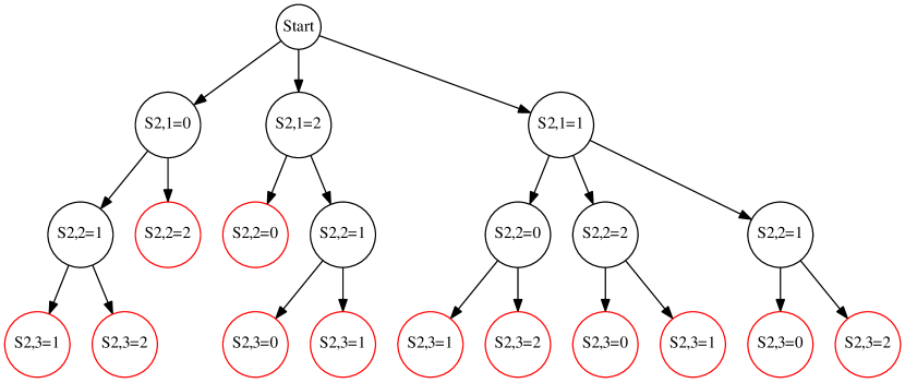
Figure 7: Decisional tree for the construction of degree-spectra matrices realizing $J$ and corresponding to pentagon graphs. The 12 leaves of the tree are shown in red.

In order to obtain an analytical result for the weighted estimate, rather than computing the probability of occurrence of each degree-spectra matrix as sampled by our algorithm, we need to compute their actual number. From the previous subsection, we already know that all the hexagon and bow tie graphs come from the same degree-spectra matrix $S_{HB}$, which is unique. Then, we only need to compute the number of degree-spectra matrices corresponding to pentagon graphs.

To do so, remember that the first choice in the construction of a degree-spectra matrix from $J$ is the value of the element $S_{2,1}$. If $S_{2,1}=0$ or $S_{2,1}=2$, then we are guaranteed to get a pentagon graph. However, while each of these two choices fixes the value of $S_{3,1}$, we are still free to select a value for the next “free” element, $S_{2,2}$.

If $S_{2,1}=0$, the allowed values for $S_{2,2}$ are 1 and 2. Choosing 2 fixes all the other elements of the degree-spectra matrix. Conversely, choosing 1 results in $S_{2,3}$ still to be determined. Its possible values are 1 and 2. Thus, there are 3 different degree-spectra matrices with $S_{2,1}=0$.

If, instead, $S_{2,1}=2$, the situation is very similar to the first case. The possible choices for $S_{2,2}$ are 0 and 1. Choosing 0 fixes the entire matrix; choosing 1 requires to select a value for $S_{2,3}$, which can be either 0 or 1. Thus, there are 3 matrices with $S_{2,1}=2$.

The third possibility of $S_{2,1}=1$ still allows degree-spectra matrices corresponding to a pentagon graph. Similarly to the previous case, the simplest way to construct one is to impose $S_{2,2}=0$ or $S_{2,2}=2$. In both cases, one must then choose a value for $S_{2,3}$. The possibilities are 1 and 2, if $S_{2,2}=0$, or 0 and 1, if $S_{2,2}=2$. Any choice for $S_{2,3}$ fixes all the remaining elements of the matrix.

Finally, it is still possible to choose $S_{2,1}=1$ and $S_{2,2}=1$, and still construct matrices corresponding to a pentagon graph. The choice is again on $S_{2,3}$. Choosing $S_{2,3}=0$ or $S_{2,3}=2$ fixes all the other elements of the matrix, whose realizations will be pentagon graphs. Imposing $S_{2,3}=1$, instead results in the matrix $S_{HB}$, exhausting all possibilities. This shows that there are 6 different matrices with $S_{2,1}=1$ that generate pentagon graphs.

The decisional tree we just described is shown in Fig. 7 as a visual aid. In summary, there are 12 different degree-spectra matrices that realize $J$ and whose realizations are always pentagon graphs. Knowing $\left\langle c_{2}\right\rangle_{P}$, $\left\langle c_{3}\right\rangle_{P}$, $\left\langle c_{2}\right\rangle_{HB}$ and $\left\langle c_{3}\right\rangle_{HB}$, which we computed before, we can finally calculate the weighted average clustering coefficients:

$$\left\langle c_{2}\right\rangle_{weighted} =\frac{12}{13}\cdot\frac{1}{4}+\frac{1}{13}\cdot{1}{3}=\frac{10}{39}$$ (37)

$$\left\langle c_{3}\right\rangle_{weighted} =\frac{12}{13}\cdot\frac{1}{3}+\frac{1}{13}\cdot{1}{9}=\frac{37}{117}\>.$$ (38)

B.3 Numerical verification

To validate our algorithm against the analytical results presented in the two subsections above, we performed extensive numerical simulations, generating $10^{4}$ degree-spectra matrices, and $10^{4}$ samples per matrix, for a total of $10^{8}$ graphs. For each graph generated, we saved the average local clustering coefficients for nodes of both degrees. Then, we obtained both weighted and unweighted results by averaging the data first naively, and then with a proper use of the weights according to Eq. 8. The results, shown in Table 1, show that the weighted averages obtained using our algorithm converge to the correct result. Also, the difference between weighted and unweighted results can be appreciated even when it is quite small, as in our example. This illustrate the sensitivity of our method, as well as the necessity of using proper sampling when performing this kind of studies.

Table 1: Comparison between analytical and simulated averaged local clustering coefficients.

Coeff.	Theor. unweigh.	Simul. unweigh.	Theor. weigh.	Simul. weigh.
$c_{2}$	$0.25309$	$0.25320$	$0.25641$	$0.25664$
$c_{3}$	$0.32510$	$0.32483$	$0.31624$	$0.31570$

References

References

- [1] Newman M E J 2003 SIAM Review 45, 167–256
- [2] Ben-Naim E, Fraunfelder H and Toroczkai Z 2004 Complex Networks (Lecture Notes in Physics 650) (Springer)
- [3] Boccaletti S et al. 2006 Phys. Rep. 424, 175–308
- [4] Boccaletti S et al. 2014 Phys. Rep. 544, 1
- [5] Erdős P and Gallai T 1960 Mat. Lapok 11, 264–73
- [6] Havel V 1955 Časopis Pěst. Mat. 80, 477–9
- [7] Hakimi S L 1962 J. Soc. Ind. Appl. Math. 10, 496–506
- [8] Fulkerson D R 1960 Pac. J. Math. 10, 831–6
- [9] Del Genio C I, Kim H, Toroczkai Z and Bassler K E 2010 PLoS One 5, e10012
- [10] Király Z 2011 Egerváry research group on combinatorial optimization Technical report TR-2011-11 ISSN 1587–4451
- [11] Kim H, Del Genio C I, Bassler K E and Toroczkai Z 2012 New J. Phys. 14, 023012
- [12] Hell P and Kirkpatrick D G 2009 Discr. Math. 309, 5703–13
- [13] Taylor R 1982 SIAM J. Algebra. Discr. 3, 114–21
- [14] Rao A R, Jana R and Bandyopadhyay S 1996 Indian J. Stat. 58, 225–42
- [15] Kannan R, Tetali P and Vempala S 1999 Random Struct. Algor. 14, 293–308
- [16] Viger F and Latapy M 2005 in Lecture notes in computer science, vol. 3595 (Proceedings of the Annual International Conference on Computing and Combinatorics) (Berlin: Springer), 440–9
- [17] Newman M E J, Strogatz S H and Watts D J 2001 Phys. Rev. E 64, 026118
- [18] Boguñá M, Pastor-Satorras R and Vespignani A 2004 Eur. Phys. J. B 38, 205–9
- [19] Catanzaro M, Boguñá M and Pastor-Satorras R 2005 Phys. Rev. E 71, 027103
- [20] Serrano M A and Boguñá M 2005 AIP Conf. Proc. 776 (Proceedings of the International Conference on Sciences of Complex Networks), 101–7
- [21] Britton T, Deijfen M and Martin-Löf A 2006 J. Stat. Phys. 124, 1377–97
- [22] Cooper C, Dyer M and Greenhill C 2007 Comb. Probab. Comput. 16, 557–93
- [23] Greenhill C 2011 Elec. J. Combin. 16(4), 557–593
- [24] Miklós I , Erdős P L and L. Soukup 2013 Elec. J. Combin. 20(1), 16
- [25] Erdős P L, Király Z and Miklós I 2013 Comb. Prob. Comput. 22(3), 366–383
- [26] Erdős PL, Miklós I and Toroczkai Z 2015 SIAM J. Discr. Math. in press.
- [27] Molloy M and Reed B 1995 Random Struct. Algorithms 6, 161–80
- [28] Molloy M and Reed B 1998 Combinatorics, Probab. Comput. 7, 295–306
- [29] Bender E and Canfield R 1978 J. Comb. Theory A 24, 296307
- [30] Bollobás B 1980 European J. Combin. 1, 311-6
- [31] Klein-Hennig H and Hartmann A K 2012 Phys. Rev. E 85, 026101 (2012)
- [32] Kim H, Toroczkai Z, Erdős P, Miklós I and Székely L 2009 J. Phys. A: Math. Theor. 42, 392001
- [33] Erdős PL, Miklós I and Toroczkai Z 2010 Electron. J. Comb. 17, R66
- [34] Blitzstein J, Diaconis P 2010 Internet Math. 6, 489–522
- [35] Molnár F, Sreenivasan S, Szymanski B K and Korniss G 2013 Sci. Rep. 3, 1736
- [36] Pastor-Satorras R, Vázquez A, Vespignani A 2001 Phys. Rev. Lett. 87, 258701
- [37] Pearson K 1895 P. R. Soc. London 58, 240–2
- [38] Yule G U 1910 An introduction to the theory of statistics (London: Griffin)
- [39] Kendall M 1938 Biometrika 30 81–9
- [40] Newman M E J 2002 Phys. Rev. Lett. 89, 208701
- [41] Maslov S and Sneppen K 2002 Science 296, 910–3
- [42] Newman M E J 2003 Phys. Rev. E 67, 026126
- [43] Eubank S, et al. 2004 Nature 429, 180–4
- [44] D’Agostino G, Scala A and Caldarelli G 2012 EPL 97, 68006
- [45] Del Genio C I and House T 2013 Phys. Rev. E 88, 040801(R)
- [46] Youssef M, Khorramzadeh Y and Eubank S 2013 Phys. Rev. E 88, 052810
- [47] Williams O and Del Genio C I 2014 PLoS One 9, e110121
- [48] Patrinos A N and Hakimi S L 1976 Discrete Math. 15, 347–58
- [49] Stanton I and Pinar A 2012 J. Exp. Alg. 17, 3.5
- [50] Czabarka É, Dutle A, Erdős P and Miklós 2015 Discr. Appl. Math. 181, 283–288
- [51] Del Genio C I, Gross T and Bassler K E 2011 Phys. Rev. Lett. 107, 178701
- [52] Gjoka M, Tillman B and Markopoulou A 2015 IEEE INFOCOM 15 Conference to be presented