Cross-Order Integral Relations from Maximal Cuts

Abstract

We study the ABDK relation using maximal cuts of one- and two-loop integrals with up to five external legs. We show how to find a special combination of integrals that allows the relation to exist, and how to reconstruct the terms with one-loop integrals squared. The reconstruction relies on the observation that integrals across different loop orders can have support on the same generalized unitarity cuts and can share global poles. We discuss the appearance of nonhomologous integration contours in multivariate residues. Their origin can be understood in simple terms, and their existence enables us to distinguish contributions from different integrals. Our analysis suggests that maximal and near-maximal cuts can be used to infer the existence of integral identities more generally.

I Introduction

The development of on-shell methods UnitarityFormalism ; GeneralizedUnitarityZqqgg ; GeneralizedUnitarityBCF ; GeneralizedUnitarityBMST ; BCFW ; LoopRecursion ; OnShellReview for computing scattering amplitudes in quantum field theory has led to rapid progress in numerous directions in recent years, including higher-loop computations in the maximally supersymmetric ($\mathcal{N}=4$) Yang–Mills theory (MSYM) ABDK ; TwoLoopFivePointEven ; ABDK5 ; HigherLoopN=4base ; Bern:2007ct ; HigherLoopN=4results ; RemainderFunction ; HigherLoopN=4misc ; HigherLoopN=4remainder ; HigherLoopN=4cluster ; HigherLoopN=4extra , the understanding of dual conformal DualConformal and Yangian Yangian symmetries, the development of alternate viewpoints on amplitudes such as twistor strings Twistors and Grassmannians GrassmanniansI ; MergeAndSplit ; GrassmanniansII , as well as the development of numerical one-loop libraries BlackHatI ; CutTools ; GoSam ; OpenLoops ; NGluon applied to next-to-leading order (NLO) calculations for phenomenology at CERN’s Large Hadron Collider. Related developments include computations at strong Yang–Mills coupling StrongCoupling , at all values of the coupling BridgingI ; BridgingII ; BridgingIII , computations of the infrared structure of amplitudes IRstructure and nonabelian exponentiation Webs , and advances in the computation of integrals out of which amplitudes are built Integrals .

Several years ago, Bern, Dixon, and Smirnov (BDS) wrote down a remarkable conjecture BDS , namely that the planar part of all maximally helicity-violating (MHV) amplitudes in $\mathcal{N}=4$ supersymmetric Yang–Mills theory can be written in a certain sense as exponentials of the one-loop amplitude,

$$1+\sum_{L=1}^{\infty}a^{L}M_{n}^{(L)}(\{s_{ij}\};\epsilon)=\exp\biggl{[}\sum_{l=1}^{\infty}a^{l}\Bigl{(}f^{(l)}(\epsilon)M_{n}^{(1)}(\{s_{ij}\};l\epsilon)+C^{(l)}+E_{n}^{(l)}(\epsilon)\Bigr{)}\biggr{]}\,,$$ (1)

where $M_{n}^{(L)}$ is the $n$-point $L$-loop MHV leading-color ordered amplitude after removing a factor of the tree color-ordered amplitude, and $a_{s}$ is a rescaled version of the Yang–Mills coupling squared. The additional functions $f^{(l)}$, $C^{(l)}$, and $E_{n}^{(l)}$ are independent of the external kinematics, and the first two are independent of the number of legs $n$. The conjecture is true for the four- and five-point functions DualConformal ; WilsonAmplitudeDuality , but fails for six or more external legs. Its failure has been a stimulus to striking advances HigherLoopN=4remainder in understanding the left-over, ‘remainder’ terms RemainderFunction .

The BDS conjecture was in turn based on an earlier calculation of the two-loop four-point amplitude ABDK by Anastasiou, Bern, Dixon, and one of the present authors (ABDK). These authors found by direct calculation that,

$$M_{4}^{(2)}(s,t;\epsilon)=\frac{1}{2}\Bigl{[}M_{4}^{(1)}(s,t;\epsilon)\Bigr{]}^{2}+f^{(2)}(\epsilon)M_{4}^{(1)}(s,t;2\epsilon)+C^{(2)}+{\cal O}(\epsilon)\,,$$ (2)

where $f^{(2)}(\epsilon)=-(\zeta_{2}+\zeta_{3}\epsilon+\zeta_{4}\epsilon^{2}+\cdots)$ and $C^{(2)}=-\zeta_{2}^{2}/2$.

Our aim in this paper is to examine this relation within the context of two-loop maximal generalized unitarity, another development of recent years in the domain of scattering amplitudes. The goal of the two-loop unitarity program is to enable theorists to go beyond NLO calculations in order to meet the challenge of future precision measurements at the LHC. Here we will instead examine an application in the context of maximally supersymmetric Yang–Mills theory.

The unitarity and generalized unitarity methods UnitarityFormalism ; GeneralizedUnitarityZqqgg ; GeneralizedUnitarityBCF ; GeneralizedUnitarityBMST ; UnitaritySupplemental ; OtherUnitarity ; BCFCutConstructible ; OPP ; Forde ; Badger ; DdimensionalII ; BFMassive ; BergerFordeReview ; Bern:2010qa at one loop have made many previously-inaccessible calculations feasible. Of particular note are processes with many partons in the final state. In its modern form of generalized unitarity, it can be applied either analytically or purely numerically EGK ; BlackHatI ; CutTools ; MOPP ; Rocket ; BlackHatII ; CutToolsHelac ; Samurai ; WPlus4 ; NGluon ; MadLoop ; GoSam . In its numerical form, the formalism underlies recent software libraries and programs used for LHC phenomenology. In this approach, the one-loop amplitude in a quantum field theory is written as a sum over a set of basis integrals, with coefficients that are rational in external spinor variables,

$${\rm Amplitude}=\sum_{j\in{\rm Basis}}{\rm coefficient}_{j}\times{\rm Integral}_{j}+{\rm Rational}\,.$$ (3)

The integral basis for one-loop amplitudes with massless internal lines contains box, triangle, and bubble integrals (dropping all terms of $\mathcal{O}(\epsilon)$ in the dimensional regulator). The coefficients are calculated from products of tree amplitudes, typically by performing contour integrals (numerically, via discrete Fourier projection). In the Ossola–Papadopoulos–Pittau (OPP) approach OPP , this decomposition is carried out at the integrand level rather than at the level of integrated expressions.

Higher-loop amplitudes can also be written in a form similar to that given in eq. (3). As at one loop, one can carry out such a decomposition at the level of the integrand. This generalization of the OPP approach has been pursued by Mastrolia and Ossola MastroliaOssola and collaborators, and also by Badger, Frellesvig, and Zhang BadgerFZ . The reader should consult refs. Zhang:2012ce ; Mastrolia:2012an ; Kleiss:2012yv ; Mastrolia:2012wf ; Mastrolia:2012du ; Huang:2013kh ; Mastrolia:2013kca for further developments within this approach. Arkani-Hamed, Bourjaily, Cachazo, Caron-Huot, and Trnka have developed an integrand-level approach AllLoopIntegrand1 ; AllLoopIntegrand2 specialized to planar contributions to the $\mathcal{N}=4$ supersymmetric theory, but to all loop orders. In ref. AllLoopIntegrand2 , these authors used global residues to study the cancellation of the $1/\epsilon^{4}$ poles in the argument of the exponential in eq. (1). The present paper can be thought of as extending this study to some of the less-singular and finite terms.

Within the unitarity method applied at the level of integrated expressions, one can distinguish two basic approaches. In a ‘minimal’ application of generalized unitarity, used in a number of prior applications Bern:1997nh ; ABDK ; BDS ; ABDK5 ; HigherLoopN=4base ; RemainderFunction ; Kosower:2010yk ; Bern:2011rj and currently pursued by Feng and Huang Feng:2012bm , one cuts just enough propagators to break apart a higher-loop amplitude into a product of disconnected tree amplitudes. Maximal cuts without complete localization of integrands have also been used in recent multi-loop calculations in maximally supersymmetric gauge and gravity theories Bern:2007ct ; Bern:2008pv ; LeadingSingularity ; Bern:2010tq ; Carrasco:2011hw ; Carrasco:2011mn ; Bern:2012uc .

We will work within a maximal unitarity approach, cutting all propagators in a given integral, and further seeking to localize integrands onto global poles to the extent possible. In principle, this allows one to isolate individual integrals on the right-hand side of the higher-loop analog of eq. (3). The coefficients are ultimately given in terms of linear combinations of multivariate residues, by so-called generalized discontinuity operators (GDOs). In previous papers TwoLoopMaximalUnitarityI ; ExternalMasses ; FourMass ; NonPlanarDoubleBox ; MassiveNonPlanarDoubleBoxes ; DoubledPropagators ; ThreeLoopLadder , the present authors and other collaborators have shown how to use multidimensional contours around global poles to extract the coefficients of both planar and nonplanar double-box master integrals, and those of three-loop ladder integrals. The same approach, with the addition of integration over non-trivial cycles, also allows the extraction of coefficients of a two-loop double box with internal masses MaximalElliptic .

We devote several sections to background material. In the next section, we review the notion of multivariate residues. We emphasize the differences from residues in a single complex variable, and provide both a geometric and algebraic picture of the most important difference, the contour dependence of such residues. In Sec. III, we review the class of two-loop planar integrals whose residues we will study later on. In Sec. IV, we review the global poles of the double-box integral. We discuss the existence of global poles shared between different double-box integrals in Sec. V, and distinguish between different ways this can happen in Sec. VI. We then analyze the four-point ABDK relation in Sec. VII, and the five-point relation in Sec. VIII. We summarize in Sec. IX.

II Multivariate Residues

The theory of multivariate complex residues is an important mathematical tool in the higher-loop generalized unitarity program. It does not always generalize naïvely from ordinary residues in a single complex variable. For the benefit of those readers who may not be familiar with the multivariate case, we give a bit of background and also discuss some of the subtleties that arise. The reader may find a more complete and mathematically rigorous presentation in the classic book of Griffiths and Harris GriffithsHarris , as well as in books of Tsikh Tsikh and Shabat Shabat . Cattani and Dickenstein CattaniDickenstein discuss the evaluation of multivariate residues from a practical point of view, making use of powerful tools from modern commutative algebra. In Sec. II.3, we show how to use one of the techniques they describe.

II.1 General Aspects

The Feynman rules for a quantum field theory tell us that the integrand at any loop order is a rational function of the loop momenta. Accordingly we can restrict attention to rational functions, in this case rational functions of several complex variables. We consider separately a numerator polynomial $h$ and a multi-factor denominator polynomial $f$, which we treat as a vector of polynomials. In more mathematical language, we take $f$ to be a holomorphic map from $\mathbb{C}^{n}\to\mathbb{C}^{n}$, and $h$ from $\mathbb{C}^{n}\to\mathbb{C}$. We are interested in global poles $\xi$, where $f$ has an isolated zero — that is, $f_{1}(\xi)=\cdots=f_{n}(\xi)=0$ and $f^{-1}(0)\cap U=\{\xi\}$ for a sufficiently small neighborhood $U$ of $\xi$. The object whose residue we want to compute at the global pole $z=\xi$ is the meromorphic $n$-form,

$$\omega=\frac{h(z)dz_{1}\wedge\cdots\wedge dz_{n}}{f_{1}(z)\cdots f_{n}(z)}\;.$$ (4)

The multivariate residue is defined by a multidimensional generalization of a contour integral: an integral taken over a product of $n$ circles, that is an $n$-torus,

$$\mathop{\rm Res}{}_{\{f_{1},\dots,f_{n}\},\xi}(\omega)=\frac{1}{(2\pi i)^{n}}\oint_{\Gamma_{\epsilon}}\frac{h(z)dz_{1}\wedge\cdots\wedge dz_{n}}{f_{1}(z)\cdots f_{n}(z)}\;,$$ (5)

where $\Gamma_{\delta}=\{z\in\mathbb{C}^{n}:|f_{i}(z)|=\delta_{i}\}$ and the $\delta_{i}$ have infinitesimal real values. The definition of $\Gamma_{\delta}$ is the first difference from single-variable contour integration, as the integration cycle is defined not directly in terms of the variables $z$ but rather in terms of the denominator factors $f_{i}(z)$.

The simplest case is the factorizable one: if each component of $f$ depends only on a single variable, that is $f_{i}(z)=f_{i}(z_{i})$, the residue factorizes completely into a product of one-dimensional contour integrals,

$$\mathop{\rm Res}{}_{\{f_{1},\dots,f_{n}\},\xi}(\omega)=\frac{1}{(2\pi i)^{n}}\oint_{|f_{1}(z_{1})|=\delta_{1}}\frac{dz_{1}}{f_{1}(z_{1})}\cdots\oint_{|f_{n}(z_{n})|=\delta_{n}}\frac{dz_{n}}{f_{n}(z_{n})}h(z)\;.$$ (6)

In general, however, each $f_{i}$ will depend on several variables. There are two types of multivariate residues we should consider: nondegenerate and degenerate. In this case, to compute the residue we must first evaluate the Jacobian determinant,

$$J(\xi)\equiv\det_{i,j}\left(\frac{\partial f_{i}}{\partial z_{j}}\right)\bigg{|}_{z=\xi}\;.$$ (7)

So long as this Jacobian does not vanish, the residue is said to be nondegenerate. For a nondegenerate residue, we can apply a coordinate transformation to eq. (5) in order to factorize the denominator in a small neighborhood of the global pole. We can do so, for example, by making use of the transformation law presented and proved in Sec. 5.1 of ref. GriffithsHarris :

Let $I=\langle f_{1}(z),\ldots,f_{n}(z)\rangle$ be a zero-dimensional ideal generated by a finite set of meromorphic functions $f_{i}(z):\mathbb{CP}^{n}\to\mathbb{C}$ with $f_{i}(\xi)=0$. Furthermore, let $J=\langle g_{1}(z),\ldots,g_{n}(z)\rangle$ be a zero-dimensional ideal such that $J\subseteq I$; that is, whose generators are related to those of $I$ by $g_{i}(z)=\sum_{i=1}^{n}a_{ij}(z)f_{j}(z)$ with the $a_{ij}(z)$ being polynomials. Letting $A(z)=(a_{ij}(z))_{i,j=1,\ldots,n}$ denote the conversion matrix, the residue at $\xi$ satisfies,

$$\mathop{\mathrm{Res}}_{\{f_{1},\ldots,f_{n}\},\hskip 0.85358pt\xi}\left(\frac{h(z)\hskip 1.13809ptdz_{1}\wedge\cdots\wedge dz_{n}}{f_{1}(z)\cdots f_{n}(z)}\right)\hskip 2.84526pt=\hskip 2.84526pt\mathop{\mathrm{Res}}_{\{g_{1},\ldots,g_{n}\},\hskip 0.85358pt\xi}\left(\frac{h(z)\hskip 0.28453pt\det A(z)\hskip 1.13809ptdz_{1}\wedge\cdots\wedge dz_{n}}{g_{1}(z)\cdots g_{n}(z)}\right)\,.$$ (8)

After the transformation, we obtain,

$$\mathop{\rm Res}{}_{\{f_{1},\dots,f_{n}\},\xi}(\omega)=\frac{1}{(2\pi i)^{n}}\frac{h(\xi)}{J(\xi)}\;.$$ (9)

for the nondegenerate residue. On the other hand, if the Jacobian vanishes, the residue is termed degenerate. In this case, the transformation law (8) remains valid GriffithsHarris and may be used to compute the residue. To find a useful transformation of the set of ideal generators, we follow the approach explained in Sec. 1.5.4 of ref. CattaniDickenstein (see also applications by one of the present authors and Zhang ThreeLoopLadder ; DoubledPropagators ; MassiveNonPlanarDoubleBoxes ). The idea is to choose the $g_{i}$ to be univariate; that is, $g_{i}(z_{1},\ldots,z_{n})=g_{i}(z_{i})$ so that the residue can be evaluated as a product of univariate residues. A set of univariate polynomials $g_{i}$ can be obtained by generating a Gröbner basis Buchberger of $\{f_{1}(z),\ldots,f_{n}(z)\}$ in lexicographic monomial order. (The reader may consult the books in ref. ComputationalAlgebraicGeometry for background material on multivariate polynomials and Gröbner bases.) Specifying the variable ordering $z_{i+1}\succ z_{i+2}\succ\cdots\succ z_{n}\succ z_{1}\succ z_{2}\cdots\succ z_{i}$ will produce a Gröbner basis containing a polynomial which depends only on $z_{i}$. We define $g_{i}(z_{i})$ as this polynomial. By considering all $n$ cyclic permutations of the variable ordering $z_{1}\succ z_{2}\succ\cdots\succ z_{n}$ we thus generate a set of $n$ univariate polynomials $\{g_{1}(z_{1}),\ldots,g_{n}(z_{n})\}$.

If the number of denominator factors of the form $\omega$ is greater than the number of variables $n$, we partition the denominator of $\omega$ into $n$ factors. For a given pole $\xi$, any partitioning $\{f_{1},\ldots,f_{n}\}$ which generates a zero-dimensional ideal produces an a priori distinct residue. We will see an example of this in the next subsection.

Degenerate residues will play an important role in the present paper. In the next subsection, we consider a simple example of a degenerate residue, give a geometric picture, and show how to evaluate it both geometrically and algebraically.

II.2 Geometry of Degenerate Residues

Let us consider the following two-form,

$$\omega=\frac{z_{1}dz_{1}\wedge dz_{2}}{z_{2}(a_{1}z_{1}+a_{2}z_{2})(b_{1}z_{1}+b_{2}z_{2})}\;.$$ (10)

For generic values of the $a_{i}$ and $b_{i}$, there is a single global pole at finite values of $z_{1}$ and $z_{2}$: requiring any two of the denominator factors to vanish yields the solution $z_{1}=z_{2}=0$. We immediately see that all three factors vanish at the global pole, and that the two-dimensional residue at the global pole is degenerate according to the definition given in the previous subsection. In this subsection we focus on providing a more geometric picture for this example. As we shall see, the global pole admits two distinct integration contours, which yield distinct residues. This is very much unlike contour integration in one complex variable, where a contour either encloses a pole or doesn’t, and there is a unique nonzero value for a residue.

We can split the two-form into two terms by making the following change of variables in eq. (10),

$$z_{1}^{\prime}=a_{1}z_{1}+a_{2}z_{2},\quad z_{2}^{\prime}=z_{2}\;;$$ (11)

the form then becomes (dropping the primes on $z_{i}^{\prime}$),

$$\omega=\frac{1}{a_{1}}\left(\frac{1}{z_{2}(c_{1}z_{1}+c_{2}z_{2})}-\frac{a_{2}}{z_{1}(c_{1}z_{1}+c_{2}z_{2})}\right)dz_{1}\wedge dz_{2}\;,$$ (12)

where $c_{1}\equiv b_{1}$ and $c_{2}\equiv a_{1}b_{2}-a_{2}b_{1}$. (This separation is a partial fractioning followed by a change of variables.) Let us start by examining the first term. The canonical integration contour is a product of two circles,

$$|z_{2}|=\delta_{2}\;,\quad|c_{1}z_{1}+c_{2}z_{2}|=\delta_{c}\;,$$ (13)

where $\delta_{2},\delta_{c}>0$. The residue of this term is,

$$\frac{1}{a_{1}b_{1}(2\pi i)^{2}}\,,$$ (14)

independent of the precise values of the radii of the circles. Going into a little bit more detail, we can parametrize the integration cycle as

$$z_{2}=\delta_{2}e^{i\theta_{2}}\;,\quad c_{1}z_{1}+c_{2}z_{2}=\delta_{c}e^{i\theta_{c}}\;,$$ (15)

so that, as $\theta_{2},\theta_{c}$ run over the interval $[0,2\pi]$ the cycle is traced out. (Indeed, the contour integrals become ordinary integrals over $\theta_{2},\theta_{c}$.)

What about the second term of eq. (12)? Care must be taken to ensure that the integrand is not singular on the contour; that would be an illegitimate contour. The second denominator factor is of course nonvanishing on the cycle (15). We can use the same pair of equations to write

$$z_{1}=(\delta_{c}e^{i\theta_{c}}-c_{2}\delta_{2}e^{i\theta_{2}})/c_{1}\;.$$ (16)

It follows that $z_{1}$ (the first denominator factor) will not vanish so long as $\delta_{c}\neq|c_{2}|\delta_{2}$. On the other hand, if $\delta_{c}=|c_{2}|\delta_{2}$, $z_{1}$ is guaranteed to vanish for some values of the angles. The illegitimate choice $\delta_{c}=|c_{2}|\delta_{2}$ divides the moduli space $(\delta_{c},\delta_{2})$ into two regions,

$$\mathrm{(1)}\hskip 7.11317pt\delta_{c}>|c_{2}|\delta_{2}\hskip 19.91692pt\mathrm{and}\hskip 19.91692pt\mathrm{(2)}\hskip 7.11317pt\delta_{c}<|c_{2}|\delta_{2}\;,$$ (17)

which we consider in turn.

At a first glance, the global contour (15) winds around $z_{1}=0$ in both regions. However, in the first region, it is the $\theta_{c}$-parametrized circle which winds around this point; the $\theta_{2}$-parametrized circle does not enclose $z_{1}=0$. But $\theta_{c}$ is the same variable which winds around the zero of the second denominator factor; that is, it is not linearly independent. This means that the torus fails to have the global pole inside it; the situation is more like a tube with the global pole sitting at the center of the symmetry plane of the tube, but not inside the tube. We conclude that in region (1), the second term in eq. (12) integrated over the cycle (15) produces a vanishing residue. In contrast, in region (2), the $\theta_{2}$-parametrized circle does wind around $z_{1}=0$, so that the contour (15) will enclose the global pole of the second term in eq. (12) as well as the first. Thus, in this region, both terms produce a nonvanishing residue. In particular, we observe that the residue of eq. (12) differs in the two regions (17), and thus depends on the relative radii $\delta_{2},\delta_{c}$ of the integration cycle.

More generally, let us consider a generic torus,

$$z_{1}=\delta_{1,1}e^{i\theta_{1}}+\delta_{1,2}e^{i\theta_{2}}\;,\quad z_{2}=\delta_{2,1}e^{i\theta_{1}}+\delta_{2,2}e^{i\theta_{2}}\;,$$ (18)

where $\delta_{i,j}$ are real positive constants which fix the shape of the contour. For the $2$-form at hand, we could rescale all $\delta$s uniformly without loss of generality, so we really have only three independent real parameters.

The contour is legitimate for the first term in eq. (12) if and only if $\delta_{2,1}\neq\delta_{2,2}$ and $r_{1}\neq r_{2}$, where

$$r_{1}=|c_{1}\delta_{1,1}+c_{2}\delta_{2,1}|\hskip 17.07164pt\mathrm{and}\hskip 17.07164ptr_{2}=|c_{1}\delta_{1,2}+c_{2}\delta_{2,2}|\;.$$ (19)

The contour is legitimate for the second term if and only if $\delta_{1,1}\neq\delta_{1,2}$ and $r_{1}\neq r_{2}$. This gives us eight regions to consider, corresponding to choosing the upper or lower inequality in each of the three relations,

$$\delta_{2,1}\gtrless\delta_{2,2}\;,\quad\delta_{1,1}\gtrless\delta_{1,2}\;,\quad r_{1}\gtrless r_{2}\;.$$ (20)

Let us denote the upper choice by ‘$+$’, and the lower choice by ‘$-$’; each region is then labeled by a string of signs. We can see that in $R^{+++}$, corresponding to $\delta_{2,1}>\delta_{2,2}$, $\delta_{1,1}>\delta_{1,2}$ and $r_{1}>r_{2}$, $\theta_{1}$ is the wrapping variable for $z_{1}$ and $z_{2}$ — but also for $c_{1}z_{1}+c_{2}z_{2}$, so that the torus fails to enclose the pole in either term in eq. (12). In $R^{++-}$, the torus will enclose both terms, and the residue will be the sum of the two terms’ residues. In $R^{+-+}$, the torus encloses only the second term, and in $R^{+--}$, the torus encloses only the first term. The remaining four regions are related to these four by flipping all inequalities, which leaves the results invariant (up to a sign).

The above analysis shows that a degenerate residue is not fully characterized by the location of the pole. The value of the residue depends on the shape of the torus wrapping around the global pole. Therefore, to correctly specify a residue, we should rather think of the integration cycles. In the present example we deduced that the moduli space of tori is divided into several regions. These regions correspond to distinct homology classes of the $(z_{1},z_{2})$ space with the zeros of the individual denominator factors in (10) removed. (In the mathematics literature, the hypersurfaces where these factors vanish are called divisors.) That is, tori (18) with moduli $\delta_{i,j}$ taken from distinct regions $R^{+++},R^{++-}$, etc. are non-homologous.

II.3 Algebraic Evaluation of Degenerate Residues

Let us now turn to the evaluation of the residues of $\omega$ at the pole at $\xi=(0,0)$ by use of the approach explained at the end of Sec. II.1. This calculation serves the dual purpose of providing a concrete example of the evaluation algorithm, and of displaying a one-to-one map between the distinct denominator partitionings and the distinct regions $R^{+++},R^{++-}$, etc. of the torus moduli space discussed at the end of the previous subsection. This map provides a dictionary between the algebraic and geometric pictures of distinct residues for a form at a given global pole.

Let us denote the denominator factors of eq. (10) as follows,

$$f_{1}(z_{1},z_{2}) =z_{2}\,,$$ (21)

$$f_{2}(z_{1},z_{2}) =a_{1}z_{1}+a_{2}z_{2}\,,$$ (22)

$$f_{3}(z_{1},z_{2}) =b_{1}z_{1}+b_{2}z_{2}\,.$$ (23)

As we are performing a two-dimensional contour integral, we seek to partition the denominator (10) into two factors. This can be done in three distinct ways, namely $\{f_{1},f_{2}f_{3}\}$, $\{f_{2},f_{3}f_{1}\}$ and $\{f_{3},f_{1}f_{2}\}$. Let us evaluate the residue for the denominator partitioning $\{f_{1},f_{2}f_{3}\}$, using the method explained at the end of Sec. II.1. The lexicographically ordered Gröbner basis of $\{f_{1},f_{2}f_{3}\}$ in the variable ordering $z_{2}\succ z_{1}$ is $\{a_{1}b_{1}z_{1}^{2},z_{2}\}$; in the variable ordering $z_{1}\succ z_{2}$ it is $\{z_{2},a_{1}b_{1}z_{1}^{2}\}$. Choosing the first element of each Gröbner basis we have,

$$g_{1}(z_{1},z_{2}) =a_{1}b_{1}z_{1}^{2}\,,$$ (24)

$$g_{2}(z_{1},z_{2}) =z_{2}\,.$$ (25)

We can obtain the conversion matrix as a by-product of finding the Gröbner basis (or using the approach implemented in ref. Lichtblau ). In the simple case considered here, ordinary multivariate polynomial division yields the same result,

$$A\hskip 1.99168pt=\hskip 1.99168pt\begin{pmatrix}-(a_{1}b_{2}+a_{2}b_{1})z_{1}-a_{2}b_{2}z_{2}&\hskip 4.2679pt1\\ 1&\hskip 4.2679pt0\end{pmatrix}\,,$$ (26)

that relates the two sets of ideal generators,

$$A\cdot\hskip 1.13809pt\begin{pmatrix}f_{1}(z_{1},z_{2})\\ f_{2}(z_{1},z_{2})f_{3}(z_{1},z_{2})\end{pmatrix}=\begin{pmatrix}g_{1}(z_{1},z_{2})\\ g_{2}(z_{1},z_{2})\end{pmatrix}\,.$$ (27)

From the transformation law (8) we then find that the residue of $\omega$ at $\xi=(0,0)$ with respect to the ideal generators $\{f_{1},f_{2}f_{3}\}$ is

$$\mathop{\mathrm{Res}}_{\{f_{1},f_{2}f_{3}\},\hskip 1.42262pt\xi}\omega\hskip 2.84526pt=\hskip 2.84526pt\mathop{\mathrm{Res}}_{\xi}\frac{z_{1}\hskip 0.56905pt\det A\hskip 1.99168ptdz_{1}\wedge dz_{2}}{g_{1}(z_{1},z_{2})\hskip 1.42262ptg_{2}(z_{1},z_{2})}\hskip 2.84526pt=\hskip 2.84526pt-\mathop{\mathrm{Res}}_{\xi}\frac{dz_{1}\wedge dz_{2}}{a_{1}b_{1}z_{1}z_{2}}\,.$$ (28)

In practice, it is important to keep in mind that the residue is antisymmetric under interchanges of the denominator factors of the form $\omega$. We observe that the denominator on the right-hand side of eq. (28) is a product of univariate polynomials, as desired. The residue can therefore be computed as a product of univariate residues and yields,

$$\rho_{1}\equiv\mathop{\mathrm{Res}}_{\{f_{1},f_{2}f_{3}\},\hskip 1.42262pt\xi}\omega\hskip 2.84526pt =\hskip 2.84526pt-\frac{1}{a_{1}b_{1}(2\pi i)^{2}}\,,$$ (29)

$$\rho_{2}\equiv\mathop{\mathrm{Res}}_{\{f_{2},f_{3}f_{1}\},\hskip 1.42262pt\xi}\omega\hskip 2.84526pt =\hskip 2.84526pt-\frac{a_{2}}{a_{1}(a_{1}b_{2}-a_{2}b_{1})(2\pi i)^{2}}\,,$$ (30)

$$\rho_{3}\equiv\mathop{\mathrm{Res}}_{\{f_{3},f_{1}f_{2}\},\hskip 1.42262pt\xi}\omega\hskip 2.84526pt =\hskip 2.84526pt\frac{b_{2}}{b_{1}(a_{1}b_{2}-a_{2}b_{1})(2\pi i)^{2}}\,,$$ (31)

where the residues for the two other denominator partitionings $\{f_{2},f_{3}f_{1}\}$ and $\{f_{3},f_{1}f_{2}\}$ are computed in a similar fashion.

Likewise, we can apply the residue evaluation algorithm to each of the two terms in eq. (12) separately, yielding $\rho_{1}$ and $\rho_{2}$ for the first and second terms respectively. Combining this with the observations made in the discussion following eq. (17), we see that in the region $R^{+++}$ of the torus moduli space, the residue evaluates to $0$; in $R^{+--}$ to $\rho_{1}$; in $R^{+-+}$ to $\rho_{2}$; and in $R^{++-}$ to $\rho_{1}+\rho_{2}=-\rho_{3}$. These observations allow us to conclude that we have the following one-to-one map between the partitionings of the denominator of $\omega$ and the regions of the torus moduli space,

$$\{f_{1},f_{2}f_{3}\}\hskip 5.69054pt \longleftrightarrow\hskip 5.69054ptR^{+--}$$ (32)

$$\{f_{2},f_{3}f_{1}\}\hskip 5.69054pt \longleftrightarrow\hskip 5.69054ptR^{+-+}$$ (33)

$$\{f_{3},f_{1}f_{2}\}\hskip 5.69054pt \longleftrightarrow\hskip 5.69054ptR^{++-}\,.$$ (34)

This map provides a dictionary between the algebraic and geometric pictures of the distinct residues defined at the given global pole.

Only two out of the three residues $\rho_{1},\rho_{2},\rho_{3}$ in eqs. (29)–(31) are independent, as the residues satisfy the identity,

$$\rho_{1}+\rho_{2}+\rho_{3}=0\,.$$ (35)

In the geometric picture, only two of the regions $R^{+--},R^{+-+},\ldots$ define linearly independent integration cycles.

III Two-Loop Integrals

In this section, we introduce the principal actors in our study, planar two-loop integrals. Let us first define our notation for one-loop integrals,

$$I_{n}(K_{1},\ldots,K_{n})\equiv-i\int\frac{d^{D}\ell}{(2\pi)^{D}}\;\frac{1}{\ell^{2}(\ell-K_{1})^{2}(\ell-K_{12})^{2}\cdots(\ell-K_{1\cdots(n-1)})^{2}}\,.$$ (36)

We use the notation $K_{j\cdots l}=K_{j}+\cdots+K_{l}$.

We will make use of the massless box integral, $I_{\square}=I_{4}$, and the massless pentagon, $I_{\pentagon}=I_{5}$.

(a)

(b)

(c)

Figure 1: The three basic types of two-loop planar integrals, labeled by the number of legs attached to each internal line of the vacuum diagram: (a) $P_{n_{1},n_{2}}$, (b) $P^{*}_{n_{1},n_{2}}$, (c) $P^{**}_{n_{1},n_{2}}$.

Two-loop integrals can be organized into two broad classes: those that factor into a product of one-loop integrals when cutting certain internal lines; and those that are irreducibly two-loop, which remain connected upon cutting any internal line. We can organize irreducibly two-loop integrals, constructed by attaching external legs to the non-factorizable two-loop vacuum diagram, into three classes TwoLoopBasis . These have external legs attached to one or two of the internal lines, and possibly to its vertices. Attaching external legs to the third internal line as well (the middle line) would yield non-planar integrals, which we will not consider in the present article. We label the integrals according to the number of external legs attached to each of the vacuum diagram’s internal lines. The absence of lines attached to vertices is denoted by a superscripted star. The three types of integrals are,

$$P_{n_{1},n_{2}}[{N}(\ell_{1},\ell_{2})] =(-i)^{2}\int\frac{d^{D}\ell_{1}}{(2\pi)^{D}}\frac{d^{D}\ell_{2}}{(2\pi)^{D}}\;\frac{{N}(\ell_{1},\ell_{2})}{\ell_{1}^{2}(\ell_{1}-K_{1})^{2}\cdots(\ell_{1}-K_{1\cdots n_{1}})^{2}(\ell_{1}+\ell_{2}+K_{n_{1}+n_{2}+2})^{2}}$$

$$\hphantom{\int\frac{d^{D}\ell_{1}}{(2\pi)^{D}}\frac{d^{D}\ell_{2}}{(2\pi)^{D}}}\times\frac{1}{\ell_{2}^{2}(\ell_{2}-K_{n_{1}+n_{2}+1})^{2}\cdots(\ell_{2}-K_{(n_{1}+2)\cdots(n_{1}+n_{2}+1)})^{2}}\,,$$

$$P^{*}_{n_{1},n_{2}}[{N}(\ell_{1},\ell_{2})] =(-i)^{2}\int\frac{d^{D}\ell_{1}}{(2\pi)^{D}}\frac{d^{D}\ell_{2}}{(2\pi)^{D}}\;\frac{{N}(\ell_{1},\ell_{2})}{\ell_{1}^{2}(\ell_{1}-K_{1})^{2}\cdots(\ell_{1}-K_{1\cdots n_{1}})^{2}(\ell_{1}+\ell_{2})^{2}}$$

$$\hphantom{\int\frac{d^{D}\ell_{1}}{(2\pi)^{D}}\frac{d^{D}\ell_{2}}{(2\pi)^{D}}}\times\frac{1}{\ell_{2}^{2}(\ell_{2}-K_{n_{1}+n_{2}+1})^{2}\cdots(\ell_{2}-K_{(n_{1}+2)\cdots(n_{1}+n_{2}+1)})^{2}}\,,$$ (37)

$$P^{**}_{n_{1},n_{2}}[{N}(\ell_{1},\ell_{2})] =(-i)^{2}\int\frac{d^{D}\ell_{1}}{(2\pi)^{D}}\frac{d^{D}\ell_{2}}{(2\pi)^{D}}\;\frac{N(\ell_{1},\ell_{2})}{\ell_{1}^{2}(\ell_{1}-K_{1})^{2}\cdots(\ell_{1}-K_{1\cdots n_{1}})^{2}(\ell_{1}+\ell_{2})^{2}}$$

$$\hphantom{\int\frac{d^{D}\ell_{1}}{(2\pi)^{D}}\frac{d^{D}\ell_{2}}{(2\pi)^{D}}}\times\frac{1}{\ell_{2}^{2}(\ell_{2}-K_{n_{1}+n_{2}})^{2}\cdots(\ell_{2}-K_{(n_{1}+1)\cdots(n_{1}+n_{2})})^{2}}\,.$$

The numerator polynomial $N(\ell_{1},\ell_{2})$ is a function of the loop momenta as well as of external momenta. For the reader’s convenience, these integrals are shown in fig. 1.

We will examine the scalar ‘horizontal’ ($s$-channel) and ‘vertical’ ($t$-channel) double-box integrals,

$$I_{\text{HDB}}\equiv P^{**}_{2,2}(k_{1},k_{2},k_{3},k_{4})\,,$$ (38)

$$I_{\text{VDB}}\equiv P^{**}_{2,2}(k_{4},k_{1},k_{2},k_{3})\,.$$ (39)

The labeling of the loop momenta in later sections will not always follow eq. (37), but will be indicated in figures throughout the text.

We will also consider the dual-conformal pentabox integral, $P^{**}_{3,2}[(\ell_{1}+k_{5})^{2}]$; scalar and irreducible-numerator one-mass double-box integrals, $P^{**}_{2,2}[1](K_{12},k_{3},k_{4},k_{5})$ and $P^{**}_{2,2}[(\ell_{1}+k_{5})^{2}](K_{12},k_{3},k_{4},k_{5})$; and scalar and irreducible-numerator turtle-box integrals, $P^{*}_{2,2}[1]$ and $P^{*}_{2,2}[(\ell_{1}+k_{4})^{2}]$.

IV Global Poles of the Double-Box Integral

In this section, we review the global poles of the massless double-box integral. In order to find the global poles, we first impose the maximal cut, cutting all seven propagators. We then examine the resulting integrand to further localize the one remaining degree of freedom.

Formally, we impose the maximal cut by performing a contour integral around a sum of seven-tori encircling the solution surfaces. In practice, we do this simply by solving the on-shell equations for the seven different propagator momenta. It is easiest to do this by using the same linear parametrization as in ref. TwoLoopMaximalUnitarityI ,

$$\ell_{1}^{\mu} =\alpha_{1}k_{1}^{\mu}+\alpha_{2}k_{2}^{\mu}+\frac{s_{12}\alpha_{3}}{2\left\langle\smash{1}{\vphantom{1}}\right|{4}\left|\smash{2}{\vphantom{1}}\right]}\left\langle\smash{1}{\vphantom{1}}\right|{\sigma^{\mu}}\left|\smash{2}{\vphantom{1}}\right]+\frac{s_{12}\alpha_{4}}{2\left\langle\smash{2}{\vphantom{1}}\right|{4}\left|\smash{1}{\vphantom{1}}\right]}\left\langle\smash{2}{\vphantom{1}}\right|{\sigma^{\mu}}\left|\smash{1}{\vphantom{1}}\right]\,,$$

$$\ell_{2}^{\mu} =\beta_{1}k_{3}^{\mu}+\beta_{2}k_{4}^{\mu}+\frac{s_{12}\beta_{3}}{2\left\langle\smash{3}{\vphantom{1}}\right|{1}\left|\smash{4}{\vphantom{1}}\right]}\left\langle\smash{3}{\vphantom{1}}\right|{\sigma^{\mu}}\left|\smash{4}{\vphantom{1}}\right]+\frac{s_{12}\beta_{4}}{2\left\langle\smash{4}{\vphantom{1}}\right|{1}\left|\smash{3}{\vphantom{1}}\right]}\left\langle\smash{4}{\vphantom{1}}\right|{\sigma^{\mu}}\left|\smash{3}{\vphantom{1}}\right]\,.$$ (40)

In the original loop integral, taken along the real slice of complexified loop momenta, $\alpha_{1,2}$ and $\beta_{1,2}$ are real, while $\alpha_{3,4}$ and $\beta_{3,4}$ lie along rays in the complex plane. We will be considering general contour integrals in ${\mathbb{C}\mathbb{P}}^{4}$, for which all $\alpha_{i},\beta_{i}\in\mathbb{C}$.

Imposing the seven on-shell conditions leads to six distinct solutions TwoLoopMaximalUnitarityI . In all of them,

$$\alpha_{1}=1\,,\qquad\alpha_{2}=0\,,\qquad\beta_{1}=0\,,\qquad\beta_{2}=1\,,$$ (41)

while the other parameters take on different values,

$${\cal S}_{1}: \qquad\alpha_{3}=-\chi\,,\qquad \alpha_{4} =0\,,\qquad \beta_{3} =z\,,\qquad \beta_{4} =0\,;$$ (42)

$${\cal S}_{2}: \qquad\alpha_{3}=z\,,\qquad \alpha_{4} =0\,,\qquad \beta_{3} =-\chi\,,\qquad \beta_{4} =0\,;$$

$${\cal S}_{3}: \qquad\alpha_{3}=0\,,\qquad \alpha_{4} =-\chi\,,\qquad \beta_{3} =0\,,\qquad \beta_{4} =z\,;$$

$${\cal S}_{4}: \qquad\alpha_{3}=0\,,\qquad \alpha_{4} =z\,,\qquad \beta_{3} =0\,,\qquad \beta_{4} =-\chi\,;$$

$${\cal S}_{5}: \qquad\alpha_{3}=0\,,\qquad \alpha_{4} =z\,,\qquad \beta_{3} =-\frac{(\chi+1)(z+\chi)}{z+\chi+1}\,,\qquad \beta_{4} =0\,;$$

$${\cal S}_{6}: \qquad\alpha_{3}=z\,,\qquad \alpha_{4} =0\,,\qquad \beta_{3} =0\,,\qquad \beta_{4} =-\frac{(\chi+1)(z+\chi)}{z+\chi+1}\,.$$

We have defined $\chi=s_{14}/s_{12}$, and have labeled the remaining degree of freedom uniformly by $z$.

Performing the contour integral over the seven-torus leads to the appearance of an inverse Jacobian in the integrand for $z$,

$$J^{-1}(z)=-\frac{1}{16s_{12}^{3}\,z(z+\chi)}\,.$$ (43)

This integrand has two poles, at $z=0$ and $z=-\chi$. In addition, integrals containing powers of the loop momenta will also have poles in solutions ${\cal S}_{5,6}$ at $z=-\chi-1$. Such integrals will also have poles at $z=\infty$. We can fully localize the integrand by integrating $z$ along a contour surrounding one of these poles (or a linear combination thereof). These poles are global poles of the original double-box integrand; we could have equivalently performed a multivariate contour integral of the original integrand around an appropriately-chosen eight-torus.

At first glance, the six different solutions can be thought of as six independent complex planes; or, adding the point at infinity to each, as six independent copies of ${\mathbb{C}\mathbb{P}}^{1}\simeq S^{2}$. A simple count suggests that we have twenty global poles: three each for solutions ${\cal S}_{1,\ldots,4}$, and four each for solutions ${\cal S}_{5,6}$. This count is too hasty, because the six independent solutions do meet at global poles TwoloopContourUniqueness : the point $z=-\chi$ in solution ${\cal S}_{1}$ is the same point in the original loop-momentum variables as $z=-\chi$ in solution ${\cal S}_{2}$. Furthermore, we can make use of an independent Cauchy residue theorem for each of the solution spheres to rewrite contour integrals around $z=\infty$ in terms of a sum around the other poles. Removing these poles, and accounting for shared poles leaves us with eight independent global poles. Finding the appropriate contour for isolating the coefficients of the two master integrals $P^{**}_{2,2}[1]$ and $P^{**}_{2,2}[\ell_{1}\cdot k_{4}]$ was the subject of ref. TwoLoopMaximalUnitarityI .

In terms of the loop momenta, the two ‘exceptional’ poles at $z=-\chi-1$ in solutions ${\cal S}_{5,6}$ correspond to $\ell_{2}$ diverging. (The asymmetry between $\ell_{1}$ and $\ell_{2}$ is due to our choice of eliminating the poles at $z=\infty$, where $\ell_{1}$ diverges.) The scalar double-box integral (with no irreducible numerators inserted) does not have these poles, and so they do not contribute to the $\mathcal{N}=4$ amplitude. We will not need to consider them further in this paper.

The remaining six global poles are each shared between two solutions; we can choose to parametrize them as $z=-\chi$ in ${\cal S}_{2}$, which we denote ${\cal G}_{1}$; $z=-\chi$ in ${\cal S}_{4}$, denoted ${\cal G}_{2}$; $z=0$ in ${\cal S}_{1}$, denoted ${\cal G}_{3}$; $z=0$ in ${\cal S}_{3}$, denoted ${\cal G}_{4}$; $z=0$ in ${\cal S}_{5}$, denoted ${\cal G}_{5}$; and $z=0$ in ${\cal S}_{6}$, denoted ${\cal G}_{6}$.

The first two of these poles will be of particular interest to us. In the first (${\cal G}_{1}$),

$$\ell_{1}^{\mu} =k_{1}^{\mu}-\frac{s_{14}}{2\left\langle\smash{1}{\vphantom{1}}\right|{4}\left|\smash{2}{\vphantom{1}}\right]}\left\langle\smash{1}{\vphantom{1}}\right|{\sigma^{\mu}}\left|\smash{2}{\vphantom{1}}\right]=-\frac{\left[1\,2\right]}{2\left[2\,4\right]}\left\langle\smash{1}{\vphantom{1}}\right|{\sigma^{\mu}}\left|\smash{4}{\vphantom{1}}\right]\,,$$ (44)

$$\ell_{2}^{\mu} =k_{4}^{\mu}-\frac{s_{14}}{2\left\langle\smash{3}{\vphantom{1}}\right|{1}\left|\smash{4}{\vphantom{1}}\right]}\left\langle\smash{3}{\vphantom{1}}\right|{\sigma^{\mu}}\left|\smash{4}{\vphantom{1}}\right]=-\frac{\left\langle 3\,4\right\rangle}{2\left\langle 1\,3\right\rangle}\left\langle\smash{1}{\vphantom{1}}\right|{\sigma^{\mu}}\left|\smash{4}{\vphantom{1}}\right]\,.$$

We thus find,

$$\ell_{1}^{\mu}+\ell_{2}^{\mu}=-\frac{\left\langle 1\,3\right\rangle\left[1\,2\right]+\left\langle 3\,4\right\rangle\left[2\,4\right]}{2\left\langle 1\,3\right\rangle\left[2\,4\right]}\left\langle\smash{1}{\vphantom{1}}\right|{\sigma^{\mu}}\left|\smash{4}{\vphantom{1}}\right]=0\,.$$ (45)

The pole corresponds to the middle rung of the double box becoming soft TwoloopContourUniqueness .

The situation is similar in the second pole in the above list (${\cal G}_{2}$), which is just the spinor (or parity) conjugate of the first,

$$\ell_{1}^{\mu} =-\frac{\left\langle 1\,2\right\rangle}{2\left\langle 2\,4\right\rangle}\left\langle\smash{4}{\vphantom{1}}\right|{\sigma^{\mu}}\left|\smash{1}{\vphantom{1}}\right]\,,$$ (46)

$$\ell_{2}^{\mu} =-\frac{\left[3\,4\right]}{2\left[1\,3\right]}\left\langle\smash{4}{\vphantom{1}}\right|{\sigma^{\mu}}\left|\smash{1}{\vphantom{1}}\right]\,;$$

again $\ell_{1}^{\mu}+\ell_{2}^{\mu}=0$.

In the third pole in the above list (${\cal G}_{3}$),

$$\ell_{1}^{\mu} =-\frac{\left[1\,2\right]}{2\left[2\,4\right]}\left\langle\smash{1}{\vphantom{1}}\right|{\sigma^{\mu}}\left|\smash{4}{\vphantom{1}}\right]\,,$$ (47)

$$\ell_{2}^{\mu} =k_{4}^{\mu}\,.$$

In this case, $(\ell_{2}-k_{4})^{\mu}=0$, so it is the rung between legs 3 and 4 that becomes soft. This is also the case for the fourth pole (${\cal G}_{4}$), which is the parity conjugate of this one.

In the fifth pole in the list (${\cal G}_{5}$),

$$\ell_{1}^{\mu} =k_{1}^{\mu}\,,$$ (48)

$$\ell_{2}^{\mu} =-\frac{\left\langle 3\,4\right\rangle}{2\left\langle 1\,3\right\rangle}\left\langle\smash{1}{\vphantom{1}}\right|{\sigma^{\mu}}\left|\smash{4}{\vphantom{1}}\right]\,.$$

Here, $(\ell_{1}-k_{1})^{\mu}=0$, thus the rung between legs 1 and 2 becomes soft. This is also true for the sixth and last pole in the list (${\cal G}_{6}$), which is the parity conjugate of the fifth.

While we will not analyze the outer-rung poles ${\cal G}_{3,\ldots,6}$ in detail, they also play a role in an analysis of the ABDK relation.

V Shared Global Poles

In this section we investigate a curious phenomenon: global poles of two-loop integrals can be shared between two or more integrals. In some cases this turns out to have interesting and nontrivial consequences.

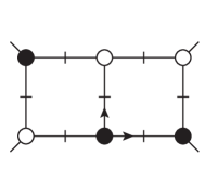
Figure 2: An example of a global pole shared between the horizontal and vertical double-box integrals. The loop momentum labeling is chosen cunningly. At the global pole, the nonvanishing heptacut propagator momentum in each double box corresponds to that of a quadruply cut one-loop box. The white and black blobs indicate chiral (MHV) and antichiral ($\overline{\text{MHV}}$) vertices, respectively, as in the conventions (for example) of ref. ExternalMasses .

V.1 Horizontal and Vertical Double Boxes

We start by re-examining the equations for the global poles in the horizontal double box,

$$\mathcal{G}_{\text{HDB}}:\;\,{} \ell_{1}^{2}=\ell_{2}^{2}=(\ell_{1}+\ell_{2}+K_{12})^{2}=(\ell_{1}-k_{4})^{2}=(\ell_{1}+\ell_{2}+k_{1})^{2}=0\;,$$

$$(\ell_{1}-K_{34})^{2}=(\ell_{1}+\ell_{2})^{2}=0\;;$$ (49)

here the labeling is not the one used earlier, but rather the one shown in fig. 2. The first five equations are identical to those for the vertical double box (again with the momentum labeling as given in fig. 2),

$$\mathcal{G}_{\text{VDB}}:\;\,{} \ell_{1}^{2}=\ell_{2}^{2}=(\ell_{1}+\ell_{2}+K_{12})^{2}=(\ell_{1}-k_{4})^{2}=(\ell_{1}+\ell_{2}+k_{1})^{2}=0\;,$$

$$(\ell_{1}+\ell_{2}-k_{4})^{2}=(\ell_{1}+k_{1})^{2}=0\;.$$ (50)

The remaining two equations in each case, on the second lines of eqs. (49) and (50), appear at first glance to be different. However, if we focus on the first two global poles (${\cal G}_{1,2}$) discussed in the previous section, we find a remarkable overlap. When the momentum of the middle rung, which in the labeling here is given simply by $\ell_{2}$, becomes soft, all the second-line equations reduce to first-line equations.

Indeed, the full set of equations simplifies to a set of four equations for $\ell_{1}$,

$$\mathcal{G}_{\text{HDB}}\Longleftrightarrow\mathcal{G}_{\text{VDB}}:\;\ell_{1}^{2}=(\ell_{1}+k_{1})^{2}=(\ell_{1}-k_{4})^{2}=(\ell_{1}+K_{12})^{2}=0\,.$$ (51)

These are precisely the quadruple-cut equations for a one-loop box with loop momentum $\ell_{1}$, labeled as in fig. 2. As is well known GeneralizedUnitarityBCF , these equations have two distinct solutions, related by spinor or equivalently parity conjugation. (One is illustrated in fig. 2.)

At first sight, the appearance of the same global pole in different integrals is alarming. There was no hint of the second integral lurking in the previous section’s discussion; its presence casts doubt on our ability to isolate the coefficient of either of the two double boxes by performing a multivariate contour integral. To understand the problem more fully, consider that both will typically contribute to a given amplitude. We can write the combined contribution together,

$$\int d^{4}\ell_{1}d^{4}\ell_{2}\left(\mathcal{I}_{\text{HDB}}N_{\text{HDB}}+\mathcal{I}_{\text{VDB}}N_{\text{VDB}}+\cdots\right)\,,$$ (52)

where $\mathcal{I}_{\text{HDB}}$ and $\mathcal{I}_{\text{VDB}}$ are the integrands of the two double-box integrals, parametrized as in fig. 2, and $N_{\text{HDB}}$ and $N_{\text{VDB}}$ are the corresponding numerators for the given amplitude. Each of the horizontal and vertical double boxes has two master integrals (one scalar and one with an irreducible numerator); following ref. TwoLoopMaximalUnitarityI , we would use a linear combination of contour integrals around the global poles to extract the corresponding coefficients in eq. (3). Each of the two horizontal master integrals, for example, has a unique contour, with the coefficient then schematically of the form,

$$\oint_{T^{8}(\mathcal{G}_{\text{HDB}})}\!d^{4}\ell_{1}d^{4}\ell_{2}\left(\mathcal{I}_{\text{HDB}}N_{\text{HDB}}+\mathcal{I}_{\text{VDB}}N_{\text{VDB}}+\cdots\right)\,.$$ (53)

The presence of a second pair of master integrals, the vertical double-box ones, risks contaminating the values of the coefficients for the horizontal double boxes. It may seem as though we cannot separate the two, because of the shared global poles.

V.2 Nonhomologous Contours

Before conceding to the alarm raised by the overlap of global poles, we should however ask whether the contours implicit in eq. (53) are the same. As we have seen in Sec. II, in the multivariate case, global poles can admit more than one inequivalent contour of integration surrounding them. (The inequivalent contours are termed nonhomologous.) As we shall see, this is precisely what happens in the case of the double boxes we are considering. Furthermore, performing the contour integrals in a certain order — a heptacut, followed by the remaining contour integration — selects one of the nonhomologous contours, and isolates the coefficient of either the horizontal or vertical double box, removing any possible contamination.

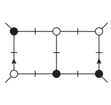
Figure 3: The horizontal and vertical double boxes. All internal lines are on-shell.

In order to visualize the multidimensional tori in question, we make use of the same parametrization as in eq. (40), but now applied to the labeling of fig. 3. This labeling allows us to align five of the seven internal lines. It also allows us to take the heptacut solutions directly from ref. TwoLoopMaximalUnitarityI .

As we saw in Sec. IV, there are six distinct heptacut solutions. Two of eight global poles are shared between the horizontal and vertical double boxes. The fully-localized integrand has a non-vanishing residue that is equal for both types of scalar double boxes, up to a sign. We now examine the possible eight-fold contours more carefully.

We first make a change of variables,

$$\alpha_{1} =\bar{\alpha}_{1}-(\chi+1)^{-1}\bar{\alpha}_{4}\,,$$ (54)

$$\alpha_{2} =\bar{\alpha}_{2}+(\chi+1)^{-1}\bar{\alpha}_{4}\,,$$

$$\alpha_{3} =\bar{\alpha}_{3}-\chi\bar{\alpha}_{\chi}+1\bar{\alpha}_{2}+\chi(\chi+1)^{-1}\bar{\alpha}_{4}-(\chi+1)^{-1}\bar{\beta}_{4}\,,$$

$$\alpha_{4} =\bar{\alpha}_{4}\,,$$

$$\beta_{1} =\bar{\beta}_{1}+(\chi+1)^{-1}\bar{\beta}_{4}\,,$$

$$\beta_{2} =\bar{\beta}_{2}-(\chi+1)^{-1}\bar{\beta}_{4}\,,$$

$$\beta_{3} =\bar{\beta}_{3}+\chi\bar{\beta}_{1}-\chi\bar{\beta}_{2}+\chi(\chi+1)^{-1}\bar{\beta}_{4}-(\chi+1)^{-1}\bar{\alpha}_{4}\,,$$

$$\beta_{4} =\bar{\beta}_{4}\,,$$

which simplifies the structure of the seven propagators. We can expand each denominator factor around the pole ${\cal G}_{1}$, retaining only the leading term in deviations $\delta\bar{\alpha}_{i}$ and $\delta\bar{\beta}_{i}$. This expansion yields the following expression for the integrand of the horizontal double box,

$$\frac{C}{\delta\bar{\alpha}_{1}\,\delta\bar{\alpha}_{2}\,\delta\bar{\alpha}_{4}\,\delta\bar{\beta}_{1}\,\delta\bar{\beta}_{2}\,\delta\bar{\beta}_{4}\,Q(\delta\bar{\alpha}_{3},\delta\bar{\beta}_{3},\delta\bar{\alpha}_{1},\delta\bar{\alpha}_{2},\delta\bar{\beta}_{1},\delta\bar{\beta}_{2})}$$ (55)

where $C$ is a function of the external spinors and invariants alone, and can be treated as a constant for the purpose of analyzing contours of integration, and where $Q$ is,

$$Q(\delta\bar{\alpha}_{3},\delta\bar{\beta}_{3},\delta\bar{\alpha}_{1},\delta\bar{\alpha}_{2},\delta\bar{\beta}_{1},\delta\bar{\beta}_{2})=\delta\bar{\alpha}_{3}\delta\bar{\beta}_{3}+\chi(\delta\bar{\alpha}_{1}-\delta\bar{\beta}_{2})(\delta\bar{\alpha}_{2}-\delta\bar{\beta}_{1})\,.$$ (56)

In principle, we should choose a cycle for each factor, but the quadratic nature of the last factor makes this less straightforward. In the region of contour moduli space where $\delta\bar{\alpha}_{3},\delta\bar{\beta}_{3}\gg\delta\bar{\alpha}_{1},\delta\bar{\alpha}_{2},\delta\bar{\beta}_{1},\delta\bar{\beta}_{2}$, the quadratic factor simplifies into the product of two linear factors ($\delta\bar{\alpha}_{3}\,\delta\bar{\beta}_{3}$), and the structure of the eight-tori encircling the global pole becomes clearer.

In this region, we can parametrize the canonical eight-torus as follows,

$$\bar{\alpha}_{1}={} \delta_{\bar{\alpha}_{1}}e^{i\theta_{\bar{\alpha}_{1}}}\,,\!\! \!\!\bar{\alpha}_{2}={} \delta_{\bar{\alpha}_{2}}e^{i\theta_{\bar{\alpha}_{2}}}\,,\!\! \!\!\bar{\alpha}_{3}={} -\chi+\delta_{\bar{\alpha}_{3}}e^{i\theta_{\bar{\alpha}_{3}}}\,,\!\! \!\!\bar{\alpha}_{4}={} \delta_{\bar{\alpha}_{4}}e^{i\theta_{\bar{\alpha}_{4}}}\,,$$

$$\bar{\beta}_{1}={} \delta_{\bar{\beta}_{1}}e^{i\theta_{\bar{\beta}_{1}}}\,,\!\! \!\!\bar{\beta}_{2}={} \delta_{\bar{\beta}_{2}}e^{i\theta_{\bar{\beta}_{2}}}\,,\!\! \!\!\bar{\beta}_{3}={} -\chi+\delta_{\bar{\beta}_{3}}e^{i\theta_{\bar{\beta}_{3}}}\,,\!\! \!\!\bar{\beta}_{4}={} \delta_{\bar{\beta}_{4}}e^{i\theta_{\bar{\beta}_{4}}}\,.$$ (57)

The $\delta$s are positive real numbers, and the angles $\theta$ run over $[0,2\pi]$ in order to cover the surface of integration. As discussed above, we take $\delta_{\bar{\alpha}_{1}},\delta_{\bar{\alpha}_{2}},\delta_{\bar{\beta}_{1}},\delta_{\bar{\beta}_{2}}\ll\delta_{\bar{\alpha}_{3}},\delta_{\bar{\beta}_{3}}$. Taking a horizontal double-box heptacut followed by a contour integration over the remaining degree of freedom $z$ corresponds to an integration over an eight-torus within this region.

Expanding each denominator factor around the same global pole for the vertical double box labeled as in fig. 3, we find

$$-\frac{C}{\delta\bar{\alpha}_{1}\,\big{(}\delta\bar{\alpha}_{3}-\delta\bar{\beta}_{4}/(\chi+1)\big{)}\,\delta\bar{\alpha}_{4}\,\delta\bar{\beta}_{1}\big{(}\delta\bar{\beta}_{3}-\delta\bar{\alpha}_{4}/(\chi+1)\big{)}\,\delta\bar{\beta}_{4}\,Q(\delta\bar{\alpha}_{3},\delta\bar{\beta}_{3},\delta\bar{\alpha}_{1},\delta\bar{\alpha}_{2},\delta\bar{\beta}_{1},\delta\bar{\beta}_{2})}$$ (58)

for the integrand, where $Q$ is the same function given in eq. (56). We first notice that if $|\chi+1|\delta_{\bar{\alpha}_{3}}=\delta_{\bar{\beta}_{4}}$ or $|\chi+1|\delta_{\bar{\beta}_{3}}=\delta_{\bar{\alpha}_{4}}$, the contour is illegitimate because the integrand is singular on it; furthermore, if $|\chi+1|\delta_{\bar{\alpha}_{3}}<\delta_{\bar{\beta}_{4}}$ or $|\chi+1|\delta_{\bar{\beta}_{3}}<\delta_{\bar{\alpha}_{4}}$, the contour fails to enclose the global pole. Thus to obtain a non-vanishing residue for the vertical double box, we must take if $|\chi+1|\delta_{\bar{\alpha}_{3}}>\delta_{\bar{\beta}_{4}}$ and $|\chi+1|\delta_{\bar{\beta}_{3}}>\delta_{\bar{\alpha}_{4}}$.

This does not suffice, however, because we also need the $Q$ factor to yield poles in $\bar{\alpha}_{2}$ and $\bar{\beta}_{2}$. This will not happen in the region where $\delta_{\bar{\alpha}_{1}},\delta_{\bar{\alpha}_{2}},\delta_{\bar{\beta}_{1}},\delta_{\bar{\beta}_{2}}\ll\delta_{\bar{\alpha}_{3}},\delta_{\bar{\beta}_{3}}$; instead, we select the region where $\delta_{\bar{\alpha}_{1}},\delta_{\bar{\alpha}_{3}},\delta_{\bar{\beta}_{1}},\delta_{\bar{\beta}_{3}}\ll\delta_{\bar{\alpha}_{2}},\delta_{\bar{\beta}_{2}}$. The vertical double-box heptacut is contained within this region, which will yield a non-zero residue for the vertical double box. Although the two integrals share the same global pole, just as in the case of the simple example considered in Sec. II, different contours surrounding the global pole are required to obtain nonvanishing residues for the two integrals.

V.3 Other Configurations of Shared Poles

The momentum labeling in fig. 2 is not the only one that gives rise to overlapping solutions of the on-shell equations. A second example of overlapping kinematical configurations is shown in fig. 4. Here, the shared global poles correspond an outer edge (again labeled $\ell_{2}$) becoming soft, $\ell_{2}^{\mu}\rightarrow 0$, in both the horizontal and vertical double boxes. One again obtains a kinematic solution for the other momentum that is identical to that of a quadruply cut one-loop box.

We could also consider a labeling where one of the integrals, say the horizontal double box, has a soft outer rung, while the vertical double box has a soft middle rung. This again gives rise to a shared global pole, where the remaining loop momentum is that of a quadruply cut one-loop box. This configuration is illustrated in fig. 5.

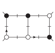
Figure 4: A second example of how a global pole could be shared between the horizontal and vertical double-box integrals.

Figure 5: A third example of how a global pole could be shared between the horizontal and vertical double-box integrals.

As we shall show in Sec. VI, the sharing described earlier in Sec. V.1 is reflected in the existence of a common daughter integral, while the two different overlaps described here do not admit a common two-loop daughter, and hence are unnatural as far as the amplitude is concerned. In later sections of this paper, we will rely only on the sharing of poles described in Sec. V.1.

V.4 Poles in the Cross-Section Integrand

The sharing of global poles displayed in figs. 4 and 5 does not have a direct application to the amplitude. It does, however, have a natural application to the differential cross section.

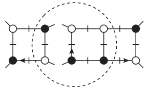
Figure 6: Two maximal unitarity cuts for diagrams that enter the cross section at the same order in the coupling: (a) a one-loop times two-loop contribution and (b) a one-loop squared contribution. These cuts share the same kinematical configuration in the indicated soft limits. The encircled subdiagrams correspond precisely to the sharing of poles illustrated in fig. 5.

We consider two contributions to the differential cross section for $2\rightarrow 2$ scattering, the interference of a one-loop amplitude with a two-loop amplitude, and the square of a five-point one-loop amplitude. Let us further consider generalized cuts of these objects. In particular, we examine the maximal cut of the horizontal double box shown in fig. 4, and multiply by the quadruple cut of the complex-conjugated four-point one-loop amplitude. This contribution is shown in fig. 6(a). This can be thought of as a global pole of the virtual contribution to the cross section. Alternatively, by the optical theorem, we can also think of it as a global pole of the four-loop amplitude for special external kinematics. From this latter point of view, the rung labeled by $\ell_{2}$ is no longer an outer rung, but instead a middle rung of a two-loop subdiagram. This subdiagram is enclosed by the dashed circle in fig. 6(a). From the analysis in the previous section we know that there is a natural candidate to cancel the pole that arises when this leg goes soft. We obtain this second contribution by replacing the horizontal double-box subdiagram by the corresponding vertical double-box subdiagram, as shown in fig. 6(b).

Returning to the interpretation of this cut as a contribution to the cross section, we see that something remarkable has happened. The individual amplitude contributions in fig. 6(b) are no longer four-point diagrams, but five-point diagrams. The additional external leg, called $k_{5}$, is soft, similar to $\ell_{2}$. The global pole is associated with either an internal line or a final-state line becoming soft, that is with infrared singularities which must ultimately cancel by the KLN theorem KLN . This cancellation echoes the cancellation of global pole residues between the two different contributions depicted in the figure. It confirms the close connection between nodal global poles and the infrared singularities of the integrated amplitude, a connection previously observed elsewhere TwoloopContourUniqueness .

VI Combining Cut Contributions

In the previous section we showed that it is possible to find kinematical configurations of loop momenta that simultaneously localize two different integrals to the same global pole. We also showed that it is nonetheless possible to find contours that distinguish the two. Of course contours that simply combine the two also exist.

In this discussion, it was important to line up the loop momenta in each integral appropriately. However, there is considerable freedom in choosing the loop-momentum parametrization. Indeed, we saw that there are different ways in which global poles can be shared between two integrals. One may wonder about the significance of any particular choice of parametrization, or equivalently any particular choice of how poles are shared.

In this section, we will argue that although the three examples in Sec. V are superficially similar, there is a clear distinction between them. The first example, shown in fig. 2, is a physically meaningful identification of loop momenta for amplitudes, whereas the second and third examples, shown in figs. 4 and 5, are not. (They nonetheless have other applications, which we discussed in the previous section.)

The examples are distinguished by the existence of daughter integrals, that is integrals with fewer propagators, which share common subsets of cuts. Their existence will allow us to align loop momenta of different integrals in a physically meaningful way, rather than in an arbitrary way. The pentacut slashed box in fig. 7 combines the horizontal and vertical double-box integrals naturally using a momentum labeling that is identical to that in fig. 2. It is possible to open the four-point vertices in the slashed box diagram in various ways with two additional propagators to obtain both the horizontal and vertical double-box integrals with massless external legs, $I_{\text{HDB}}$ and $I_{\text{VDB}}$. These integrals differ simply by a cyclic permutation of the external legs.

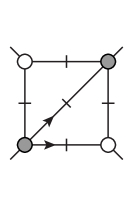
Figure 7: The pentacut provides a natural prescription for aligning the loop-momentum labels in different integrals. The global octacut poles of the double-box integrals can be analyzed by performing a further three-dimensional contour integral on the pentacut slashed-box integral at left. The gray blobs indicate vertices of indefinite chirality.

The situation is different for the other two labelings shown in figs. 4 and 5. Consider, for example, fig. 4. Can we find an integral and unitarity cut that contains both partly-cut horizontal and vertical double-box integrals? Loop momentum $\ell_{1}$ is located somewhere between external legs 1 and 4 in both integrals, so finding a unitarity cut with that property should be straightforward. However, momentum $\ell_{2}$ is located between external legs 1 and 2 in the HDB integral, but between 2 and 3 in the VDB integral. Such a behavior is difficult to reconcile in any unitarity cut. Indeed, for a planar unitarity cut it is impossible. It might conceivably be possible for a non-planar integral; but in the present paper we are in any case focused on the planar case. One could try to simultaneously reparametrize the $\ell_{2}$ dependence in both integrals so as to fit into a single unitarity cut, but there appears to be no such possibility. A similar analysis can be performed on the momentum labeling in fig. 5, leading again to the conclusion that there is no unitarity cut that is consistent with this way of sharing global poles.

We can also see the distinction between the sharing described in figs. 4 and 5 and that described in fig. 7 using dual coordinates $x_{i}$ DualConformal . The external momenta are given by differences of the coordinates, $k_{i}=x_{i+1}-x_{i}$. In terms of these coordinates, the horizontal and vertical double boxes have the following expressions,

$$I_{\text{HDB}}={} \int d^{D}x_{5}\int d^{D}x_{6}\frac{x_{13}^{4}x_{24}^{2}}{x_{15}^{2}x_{25}^{2}x_{35}^{2}x_{56}^{2}x_{36}^{2}x_{46}^{2}x_{16}^{2}}\;,$$ (59)

$$I_{\text{VDB}}={} \int d^{D}x_{5}\int d^{D}x_{6}\frac{x_{24}^{4}x_{13}^{2}}{x_{15}^{2}x_{25}^{2}x_{45}^{2}x_{56}^{2}x_{36}^{2}x_{46}^{2}x_{26}^{2}}\;.$$

Five denominators — $x_{15}^{2}$, $x_{25}^{2}$, $x_{56}^{2}$, $x_{36}^{2}$, and $x_{46}^{2}$ — are the same in both integrals. The sharing described by fig. 7 corresponds to taking the limit $x_{6}\rightarrow x_{5}$; upon taking that limit, all remaining denominators in one integral manifestly match denominators in the other ($x_{35}^{2}\leftrightarrow x_{36}^{2}$, $x_{45}^{2}\leftrightarrow x_{46}^{2}$, $x_{16}^{2}\leftrightarrow x_{15}^{2}$, and $x_{26}^{2}\leftrightarrow x_{25}^{2}$). In contrast, in the sharing described by fig. 4, the limit corresponds to taking $x_{5}\rightarrow x_{2}$ in the horizonal double box, and $x_{6}\rightarrow x_{3}$ in the vertical double box. Under this limit, only one additional denominator in each integral manifestly matches a denominator in the other: $x_{35}^{2}\leftrightarrow x_{26}^{2}$. (The remaining denominator matches only when solving the equations.) In the sharing described by fig. 5, the limit again corresponds to taking $x_{5}\rightarrow x_{2}$ in the horizonal double box, but in this case to taking $x_{5}\rightarrow x_{6}$ in the vertical double box. Here, while both additional denominators in the vertical double box manifestly match denominators in the horizontal double box, only one additional denominator in the horizontal double box matches a denominator in the vertical double box: $x_{16}^{2}\leftrightarrow x_{15}^{2}$.

VII The Four-Point ABDK Relation

We turn next to a maximal-cut analysis of the ABDK relation (2) for the four-point amplitude in the $\mathcal{N}=4$ super-Yang–Mills theory. Let us study the various integrals that arise in the two representations of the four-point amplitude on the two sides of eq. (2). In particular, we examine the integrals which admit an eight-fold localization, the one-loop box squared and the two-loop double box. They appear in the amplitude with the same power of the Yang–Mills coupling. (These integrals are also the ones of leading and equal polylogarithmic weight, whereas in the remaining terms, part of the polylogarithmic weight comes from constant prefactors.) At the very least, if we apply a GDO like that of ref. TwoLoopMaximalUnitarityI that extracts either the coefficient of the horizontal double box or of the vertical double box to the right-hand side of eq. (2), we must obtain the same coefficient as on the left-hand side. For this to be possible, both sides must share global poles. The one-loop box squared appearing on the right-hand side is of course not part of the standard basis for two-loop amplitudes, and so ordinarily one would not consider it in computing two-loop amplitudes. Furthermore, any global poles it shares with two-loop integrals would not affect our ability to extract coefficients of the latter in the standard basis. This is true even if the same contours enclose the global poles in both integrals.

As we shall see, the sharing of poles and residues is more extensive than required: the two sides share all poles and residues present in any double-box integral on the left-hand side, and on some non-maximal cut surfaces, even share integrands away from the global poles.

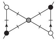
Figure 8: The bow-tie hexacut detects contributions from both the planar double box and squared one-loop boxes. This figure shows a particular example where vertices at opposite corners have equal chiralities in the bow-tie diagram.

We parametrize the squared one-loop box and horizontal double-box integrals as shown in fig. 8. We start by cutting all propagators that are manifestly shared between the two integrals. There are six such propagators, which together form the integrand of a bow-tie integral. This leads us to consider the zero locus,

$${\cal S}\equiv\big{\{}\,(\ell_{1},\ell_{2})\in{\mathbb{C}\mathbb{P}}^{4}\times{\mathbb{C}\mathbb{P}}^{4}\;|\; \ell_{1}^{2}=0\,,\;(\ell_{1}-k_{2})^{2}=0\,,\;(\ell_{1}+k_{1})^{2}=0\,,\;$$

$$\ell_{2}^{2}=0\,,\;(\ell_{2}-k_{3})^{2}=0\,,\;(\ell_{2}+k_{4})^{2}=0\,\big{\}}\,.$$ (60)

The hexacut solutions for the bow-tie are two-dimensional, parametrized by a pair of complex variables $(z_{1},z_{2})\in{\mathbb{C}\mathbb{P}}^{2}$. They are simply products of solutions for independent one-mass triangles, which makes it straightforward to write them down. There are four distinct solutions to the equations, ${\cal S}=S_{1}\cup\cdots\cup S_{4}$. We can identify four distinct hexacut diagrams which are in one-to-one correspondence with the four hexacut solutions. The diagrams are characterized by the relative chiralities of the vertices at opposite corners. By parity it suffices to work out one example of each kind: one where the chiralities at opposite corners are identical, and one where they are opposite. Performing the six-fold contour integral that imposes the hexacut conditions implicitly picks a contour that isolates only one of the horizontal or vertical double boxes, so we need not worry about sharing of global poles between these two integrals.

We can solve the on-shell equations (60) straightforwardly using the parametrization (40); they are after all just two copies of one-loop triangle cuts. We are left with one free parameter from each loop momentum. For the hexacut depicted in fig. 8, which we label ${\cal S}_{1}$, we have the very simple solution,

$${\cal S}_{1}:\,\left\{\begin{array}[]{llll}\alpha_{1}=0\,,&\;\;\alpha_{2}=0\,,&\;\;\alpha_{3}=z_{1}\,,&\;\;\alpha_{4}=0\,,\\[5.69054pt] \beta_{1}=0\,,&\;\;\beta_{2}=0\,,&\;\;\beta_{3}=z_{2}\,,&\;\;\beta_{4}=0\,.\\[2.84526pt] \end{array}\right.$$ (61)

The bow-tie hexacut squared one- and two-loop integrals then take the form,

$$I_{\text{HDB}}\big{|}_{6\text{-cut}}={} \oint d^{2}z\frac{J^{-1}(z_{1},z_{2})}{(\ell_{1}+\ell_{2}-K_{23})^{2}}\Big{|}_{{\cal S}_{1}}=-\frac{\chi}{16s_{12}^{3}}\oint\frac{d^{2}z}{z_{1}z_{2}(z_{1}+\chi)(z_{2}+\chi)}\;,$$ (62)

$$I_{\square}^{2}\big{|}_{6\text{-cut}}={} \oint d^{2}z\frac{J^{-1}(z_{1},z_{2})}{(\ell_{1}-K_{23})^{2}(\ell_{2}-K_{23})^{2}}\Big{|}_{{\cal S}_{1}}=-\frac{1}{16s_{12}^{4}}\oint\frac{d^{2}z}{z_{1}z_{2}(z_{1}+\chi)(z_{2}+\chi)}\;,$$

where $J(z_{1},z_{2})$ is the Jacobian that arises upon evaluation of the residue in the loop momentum parametrization; that is, the integrand of the scalar hexacut bow-tie integral itself. The expression $J^{-1}(z_{1},z_{2})$ is the same for all hexacut solutions,

$$J^{-1}(z_{1},z_{2})\equiv-\frac{1}{16s_{12}^{2}z_{1}z_{2}}\;.$$ (63)

We observe that, remarkably, the integrands of the horizontal double box and the squared one-loop box integrals coincide on the hexacut solution ${\cal S}_{1}$, up to a constant. Demanding that the cuts should be equal fixes the relative constant. The result takes the form,

$$s_{12}^{2}s_{23}I_{\text{HDB}}\big{|}_{6\text{-cut}}=\big{(}s_{12}s_{23}I_{\square}\big{)}^{2}\big{|}_{6\text{-cut}}\;.$$ (64)

The coefficient on the left-hand side is exactly that which appears in the four-point amplitude in the $\mathcal{N}=4$ super Yang-Mills theory (after removing overall normalization factors). Because the integrands are identical, the global poles as well as the contours surrounding them are now shared between the double-box integral and the one-loop integrals squared. What global poles are these? We find four poles, located at the following values of $(z_{1},z_{2})$,

$$(0,0)\,;\qquad(0,-\chi)\,;\qquad(-\chi,0)\,;\qquad(-\chi,-\chi)\,.$$ (65)

The first is a ‘spurious’ pole from the point of view of the double box, as it does not correspond to a maximal cut, and is thus not required for construction of the amplitude. It arises purely from the Jacobian, and corresponds to a soft limit; we will call such poles ‘soft’ poles more generally. The second pole in eq. (65) corresponds to ${\cal G}_{5}$ [eq. (48)]; the third to ${\cal G}_{3}$ [eq. (47)]; and the last pole, to ${\cal G}_{1}$ [eq. (44)]. From the point of view of the squared one-loop box, only the last pole corresponds to a maximal cut, while the first three are ‘soft’. All are nonetheless shared between the double box and the squared one-loop box. Performing the additional contour integrals to localize all coordinates of course gives us identical residues,

$$s_{12}^{2}s_{23}I_{\text{HDB}}\big{|}_{8\text{-cut}}=\big{(}s_{12}s_{23}I_{\square}\big{)}^{2}\big{|}_{8\text{-cut}}\;.$$ (66)

As mentioned earlier, this sharing does not affect our ability to extract coefficients in the two-loop version of the master equation (3), because the one-loop integrals squared are not part of the two-loop basis.

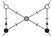
Figure 9: The second inequivalent type of bow-tie hexacut considered in the main text, with contributions from the double box and a squared box.

The parity conjugate solution to ${\cal S}_{1}$, which we label ${\cal S}_{2}$, is given by,

$${\cal S}_{2}:\,\left\{\begin{array}[]{llll}\alpha_{1}=0\,,&\;\;\alpha_{2}=0\,,&\;\;\alpha_{3}=0\,,&\;\;\alpha_{4}=z_{1}\,,\\[5.69054pt] \beta_{1}=0\,,&\;\;\beta_{2}=0\,,&\;\;\beta_{3}=0\,,&\;\;\beta_{4}=z_{2}\,.\\[2.84526pt] \end{array}\right.$$ (67)

It contains the global poles ${\cal G}_{2}$, ${\cal G}_{4}$, and ${\cal G}_{6}$, completing the list of global poles present in the horizontal double box and the equality of their residues to the squared one-loop box. Alternatively, we could examine a hexacut solution with opposite chiralities at the opposite corners, see fig. 9. The solution, which we label ${\cal S}_{3}$, takes the form,

$${\cal S}_{3}:\,\left\{\begin{array}[]{llll}\alpha_{1}=0\,,&\;\;\alpha_{2}=0\,,&\;\;\alpha_{3}=z_{1}\,,&\;\;\alpha_{4}=0\,,\\[5.69054pt] \beta_{1}=0\,,&\;\;\beta_{2}=0\,,&\;\;\beta_{3}=0\,,&\;\;\beta_{4}=z_{2}\,.\\[2.84526pt] \end{array}\right.$$ (68)

For the hexacut integrals we have

$$I_{\text{HDB}}\big{|}_{6\text{-cut}}={} -\frac{\chi+1}{16s_{12}^{3}}\oint\frac{d^{2}z}{z_{1}z_{2}\big{[}(z_{1}+\chi)(z_{2}+\chi)+z_{1}+z_{2}+\chi\big{]}}\,,$$

$$I_{\square}^{2}\big{|}_{6\text{-cut}}={} -\frac{1}{16s_{12}^{4}}\oint\frac{d^{2}z}{z_{1}z_{2}(z_{1}+\chi)(z_{2}+\chi)}\,.$$ (69)

Here, the initial six-fold contour integrals leave us with different expressions. We can nonetheless proceed as before. We know from ref. TwoLoopMaximalUnitarityI that the (horizontal) double box has two nonzero octacut poles at $(z_{1},z_{2})=(-\chi,0)$, corresponding to ${\cal G}_{3}$, and $(z_{1},z_{2})=(0,-\chi)$, corresponding to ${\cal G}_{6}$. (These poles lie on the intersection with the ${\cal S}_{1}$ and ${\cal S}_{2}$ hexacut solutions, respectively.) As before, there is also a ‘soft’ pole at $(z_{1},z_{2})=(0,0)$. (The soft pole lies on the intersection with all other hexacut solutions.) These three poles are also present in the squared one-loop integral, cf. eq. (69), where all are ‘soft’. In contrast, in this hexacut solution the global pole of the squared one-loop integral, at $(z_{1},z_{2})=(-\chi,-\chi)$ is not a global pole of the horizontal double box. Evaluating the three residues from both integrals in eq. (69) yields the same answer, up to an overall constant. For example, for the residue at $(0,0)$,

$$I_{\text{HDB}}\big{|}_{8\text{-cut}}=-\frac{1}{16\chi s_{12}^{3}}\;,\quad I_{\square}^{2}\big{|}_{8\text{-cut}}=-\frac{1}{16\chi^{2}s_{12}^{4}}\;.$$ (70)

The remaining octacut residues differ from those in eq. (70) only by an overall sign, so we will not write them down explicitly. We can summarize the results in a single equation,

$$s_{12}^{2}s_{23}I_{\text{HDB}}\big{|}_{8\text{-cut}}=\big{(}s_{12}s_{23}I_{\square}\big{)}^{2}\big{|}_{8\text{-cut}}\;.$$ (71)

To establish this identity, it would in fact suffice to take the residue at either $z_{1}=0$ or $z_{2}=0$, as the remaining heptacut integrands would be equal for the two types of integrals. A similar analysis holds for the vertical double box.

The identity of residues described above is precisely what is required for the ABDK relation (2). The right-hand side is an expression, given in terms of a physical amplitude, that has a term proportional to $I_{\square}^{2}$. The quantity $M_{4}^{(L)}$ appearing in that equation is defined in terms of the one- or two-loop partial amplitude normalized by the tree-level amplitude, $M_{4}^{(L)}(s,t;\epsilon)\equiv A_{4}^{(L)}(s,t;\epsilon)/A_{4}^{(0)}(s,t)$. The planar partial amplitudes themselves are conventionally normalized according to,

$$\mathcal{A}_{n}^{(L)}=g^{n-2}\bigg{[}\frac{2e^{-\gamma\epsilon}g^{2}N_{c}}{(4\pi)^{2-\epsilon}}\bigg{]}^{L}\sum_{\rho\in S_{n}/Z_{n}}\operatorname{Tr}(T^{a_{\rho(1)}}\cdots T^{a_{\rho(n)}})A_{n}^{(L)}(\rho(1),\dots,\rho(n))\;.$$ (72)

The removal of color and normalization factors yields $M_{4}^{(1)}(s_{12},s_{23};\epsilon)=s_{12}s_{23}I_{\square}$. We focus on the first term on the right-hand side of eq. (2), as we cannot take an eight-fold cut of the other terms; we leave them for future study. (The one-loop integral $M_{4}^{(1)}(s_{12},s_{23};2\epsilon)$ has at most a quadruple cut.) In the notation of this paper, the reduced two-loop amplitude is given by

$$M_{4}^{(2)}(s_{12},s_{23};\epsilon)=s_{12}^{2}s_{23}I_{\text{HDB}}+s_{12}s_{23}^{2}I_{\text{VDB}}\,.$$ (73)

In order to fix the numerical coefficients in front of the integrals in the ABDK relation (2), we must consider a somewhat subtle point. The term on the right-hand side of eq. (2) proportional to $I_{\square}^{2}$ is symmetric under the interchange of $\ell_{1}\leftrightarrow\ell_{2}$. The same is not true of the double-box terms on the left-hand side. These features can be seen most easily using dual coordinates DualConformal . The expressions for the double boxes were given in eq. (59); the squared one-loop box has the following expression,

$$I_{\square}^{2}={}\int d^{D}x_{5}\frac{x_{13}^{2}x_{24}^{2}}{x_{15}^{2}x_{25}^{2}x_{35}^{2}x_{45}^{2}}\int d^{D}x_{6}\frac{x_{13}^{2}x_{24}^{2}}{x_{16}^{2}x_{26}^{2}x_{36}^{2}x_{46}^{2}}\,.$$ (74)

If we antisymmetrize the right-hand side under $\ell_{1}\leftrightarrow\ell_{2}$ or equivalently $x_{5}\leftrightarrow x_{6}$, it vanishes. In contrast, the left-hand side integrand will not vanish upon antisymmetrization; it only vanishes after integration. In this respect, it is similar to integrals with insertions of Levi-Civita tensors, whose integrands (or even isolated residues) do not vanish, but which vanish after integration. We thus need to form a projector, analogous to the treatment of such insertions TwoLoopMaximalUnitarityI ; ExternalMasses ; FourMass ; NonPlanarDoubleBox ; MassiveNonPlanarDoubleBoxes ; DoubledPropagators ; ThreeLoopLadder ; MaximalElliptic , that will set the sum of residues to zero for the antisymmetric combination. It is easiest to do this by symmetrizing the left-hand side of eq. (2), and thus of eq. (71). This introduces a factor of $1/2$, because only one of the resulting two terms will have a non-vanishing octacut residue for the contour we are considering. Both terms will contribute the same result after integration along the standard contour, so the octacut relation (71) along with its partner for the vertical double box imply the following integral relation,

$$s_{12}s_{23}\big{(}s_{12}I_{\text{HDB}}+s_{23}I_{\text{VDB}}\big{)}=\frac{1}{2}\big{(}s_{12}s_{23}I_{\square}\big{)}^{2}+\text{octacut-free}\,.$$ (75)

While the double boxes do have a symmetry under interchange of $(1,2)\leftrightarrow(3,4)$, which is equivalent to $\ell_{1}\leftrightarrow\ell_{2}$, the symmetrization and resulting factor of $1/2$ are independent of the interchange symmetry, and would apply even in its absence.

Thus far we have examined only global poles present in one of the double-box integrals, and found that there is always a corresponding global pole in the one-loop box integral squared. However, one may wonder whether there are additional poles present in the squared one-loop box terms. Such poles are indeed present, at $(z_{1},z_{2})=(-\chi,-\chi)$ in the hexacut solutions ${\cal S}_{3}$ and ${\cal S}_{4}$. They occur in the product of two quadruply cut box integrals of opposite chirality. As we noted above, these poles are not global poles of the double-box integral, yet their residues are nonvanishing for the squared one-loop integral. This seeming inconsistency could perhaps be cured by inserting a parity-odd term into the integrand of the squared one-loop box in such a way as to cancel these incompatible residues. This addition would not modify the integrated expression, and hence would leave the ABDK relation (2) unmodified. We leave an investigation of this issue to future work.

VIII The Five-Point ABDK Relation

The remarkable implications of shared global poles for the four-point ABDK relation motivate a similar analysis for the five-point relation. To what extent can we reconstruct the identity from maximal cuts?

The five-point relation has the same form as the four-point one (2),

$$M_{5}^{(2)}(s_{12},s_{23},s_{34},s_{45},s_{51};\epsilon)= \frac{1}{2}\Bigl{[}M_{5}^{(1)}(s_{12},s_{23},s_{34},s_{45},s_{51};\epsilon)\Bigr{]}^{2}$$ (76)

$$+f^{(2)}(\epsilon)M_{5}^{(1)}(s_{12},s_{23},s_{34},s_{45},s_{51};2\epsilon)+C^{(2)}+{\cal O}(\epsilon)\,.$$

In this equation, the normalized five-point one-loop MSYM amplitude OneLoopFivePoint is given by,

$$M_{5}^{(1)}(\{s_{ij}\};\epsilon)=\frac{1}{4}\sum_{\rho\in\text{cyclic}}\rho(s_{34}s_{45})I_{\Square}(\rho)+\frac{\epsilon}{2}\varepsilon_{1234}I_{\pentagon}^{D=6-2\epsilon}\;,$$ (77)

where $\rho(k_{i})=k_{\rho(i)}$, $\rho(s_{ij})=s_{\rho(i)\rho(j)}$, $\varepsilon_{1234}\equiv 4i\varepsilon_{\mu\nu\rho\sigma}k_{1}^{\mu}k_{2}^{\nu}k_{3}^{\rho}k_{4}^{\sigma}$, and,

$$I_{\square}(\rho)=I_{\square}(\rho(K_{12},k_{3},k_{4},k_{5}))\,.$$ (78)

The normalized five-point two-loop MSYM amplitude ABDK5 is,

$$M_{5}^{(2)}(\{s_{ij}\}; \epsilon)=\frac{1}{8}\sum_{\rho\in\text{cyclic}}$$ (79)

$$\biggl{\{}\rho(s_{12}^{2}s_{23})P^{**}_{2,2}(\rho(k_{1},k_{2},k_{3},K_{45}))+\rho(s_{12}^{2}s_{51})P^{**}_{2,2}(\rho(k_{1},k_{2},K_{34},k_{5}))$$

$$\hskip 5.69054pt+\rho(s_{12}s_{23}s_{45})P^{**}_{3,2}[(\ell_{1}+k_{\rho(5)})^{2}](\rho(k_{1},k_{2},k_{3},k_{4},k_{5}))\biggr{\}}+\text{parity-odd}.$$

In the present paper, we will consider only the parity-even part of the amplitude. On the left-hand side of eq. (76), each pentabox and one-mass double box appears with a factor of $1/8$, whereas each square of a one-loop box appears with a factor of $1/32$, and each product of different one-loop boxes with a factor of $1/16$.

We must first work out the relevant maximal cuts of the five-point two-loop integrals that appear on the left-hand side of the five-point relation (76). In this case, we have eight propagators to cut, and so we examine the octacuts of various five-point integrals. We will again encounter several nonhomologous octacut contours that encircle the same global poles, but produce distinct residues. As in the four-point case, the sharing of global poles between different integrals plays a key role. As we shall see, the possibility of opening the four-point vertex of the turtle-box integral ($P^{*}_{2,2}$) into either the left or the right loop gives rise to a highly nontrivial sharing of global poles between different pentabox integrals ($P^{**}_{3,2}$).

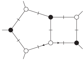
Figure 10: The four octacut solutions for the massless pentabox. In our notation, as in prior figures, chiral and antichiral vertices are depicted by white and black blobs respectively, following for example the conventions of ref. ExternalMasses . Each of these four solutions is associated with a unique point in ${\mathbb{C}\mathbb{P}}^{4}\times{\mathbb{C}\mathbb{P}}^{4}$.

VIII.1 Pentabox Global Poles

We will begin our analysis by determining the global poles of the massless pentabox integral. In four spacetime dimensions, the octacut solutions are a discrete set of points, that is, they form a zero-dimensional algebraic variety. We can localize the entire pentabox integral to discrete points in ${\mathbb{C}\mathbb{P}}^{4}\times{\mathbb{C}\mathbb{P}}^{4}$ by changing the real-slice contour to a linear combination of eight-tori each encircling one of the octacut global poles.

The global poles for the pentabox are given by the zero locus of the polynomial ideal generated by the eight inverse propagators. In our notation, this zero locus is

$${\cal S}\equiv\big{\{}(\ell_{1},\ell_{2})\in{\mathbb{C}\mathbb{P}}^{4}\!\times\!{\mathbb{C}\mathbb{P}}^{4}\;| \ell_{1}^{2}=0\,,\,(\ell_{1}\mskip-1.0mu-\mskip-1.0muk_{1})^{2}=0\,,\,(\ell_{1}\mskip-1.0mu-\mskip-1.0muK_{12})^{2}=0\,,\,(\ell_{1}\mskip-1.0mu-\mskip-1.0muK_{123})^{2}=0\,,$$ (80)

$$\ell_{2}^{2}=0\,,\,(\ell_{2}\mskip-1.0mu-\mskip-1.0muk_{5})^{2}=0\,,\,(\ell_{2}\mskip-1.0mu-\mskip-1.0muK_{45})^{2}=0\,,\,(\ell_{1}\mskip-1.0mu+\mskip-1.0mu\ell_{2})^{2}=0\,\big{\}}\,.$$

There are four inequivalent octacut solutions ${\cal S}={\cal G}_{1}\cup\cdots\cup{\cal G}_{4}$, which group into two pairs of parity conjugates. The four solutions correspond to the four ways of distributing chiral and antichiral three-point vertices in the cut pentabox diagram that are valid for generic external momenta (see fig. 10). In other words, two of the six maximal cut solutions for the one-mass four-point double-box diagram ExternalMasses fail to accommodate an additional on-shell three-point vertex for generic external kinematics.

We can solve the pentabox on-shell constraints (80) straightforwardly using the loop-momentum parametrization,

$$\ell_{1}^{\mu}={} \alpha_{1}k_{1}^{\mu}+\alpha_{2}k_{2}^{\mu}+\frac{\alpha_{3}}{2}\left\langle 1\>\!|\>\!\sigma^{\mu}\>\!|\>\!2\right]+\frac{\alpha_{4}}{2}\left\langle 2\>\!|\>\!\sigma^{\mu}\>\!|\>\!1\right]\;,$$ (81)

$$\ell_{2}^{\mu}={} \beta_{1}k_{4}^{\mu}+\beta_{2}k_{5}^{\mu}+\frac{\beta_{3}}{2}\left\langle 4\>\!|\>\!\sigma^{\mu}\>\!|\>\!5\right]+\frac{\beta_{4}}{2}\left\langle 5\>\!|\>\!\sigma^{\mu}\>\!|\>\!4\right]\;.$$

For all four solutions,

$${\cal G}_{i}:\,{} \left\{\begin{array}[]{ll}\alpha_{1}=1\,,&\;\;\alpha_{2}=0\,,\\[5.69054pt] \beta_{1}=0\,,&\;\;\beta_{2}=1\,.\end{array}\right.$$ (84)

To express the remaining parameters and for later use, it is convenient to introduce a notation for certain complex values,

$$P_{1} \equiv-\frac{\langle 1\,5\rangle}{\langle 2\,5\rangle}\;, P_{2} \equiv\frac{[2\,3]}{[1\,3]}\;, P_{3} \equiv-\frac{\langle 1\,4\rangle}{\langle 2\,4\rangle}\;,$$ (85)

$$Q_{1} \equiv-\frac{[1\,5]}{[1\,4]}\;, Q_{2} \equiv\frac{\langle 3\,4\rangle}{\langle 3\,5\rangle}\;,$$

as well as for the spinor (or parity) conjugates,

$$P^{\bullet}_{1} \equiv-\frac{[1\,5]}{[2\,5]}\;, P^{\bullet}_{2} \equiv\frac{\langle 2\,3\rangle}{\langle 1\,3\rangle}\;, P^{\bullet}_{3} \equiv-\frac{[1\,4]}{[2\,4]}\;,$$ (86)

$$Q^{\bullet}_{1} \equiv-\frac{\langle 1\,5\rangle}{\langle 1\,4\rangle}\;, Q^{\bullet}_{2} \equiv\frac{[3\,4]}{[3\,5]}\;.$$

In terms of these values, the loop-momentum parameters take on the following values at the octacut global poles of the pentabox,

$${\cal G}_{1}:{} \left\{\begin{array}[]{lrl}\alpha_{3}=0\,,\hphantom{{}_{2}^{\bullet}\,}&\;\;\alpha_{4}&=P_{2}\,,\\[5.69054pt] \beta_{3}=0\,,&\;\;\beta_{4}&=Q_{1}\,,\end{array}\right. {\cal G}_{2}:{} \left\{\begin{array}[]{lrl}\alpha_{3}=P^{\bullet}_{2}\,,&\;\;\alpha_{4}&=0\,,\\[5.69054pt] \beta_{3}=Q^{\bullet}_{1}\,,&\;\;\beta_{4}&=0\,,\end{array}\right.$$ (87)

$${\cal G}_{3}:{} \left\{\begin{array}[]{lrl}\alpha_{3}=P^{\bullet}_{2}\,,&\;\;\alpha_{4}&=0\,,\\[5.69054pt] \beta_{3}=0\,,&\;\;\beta_{4}&=Q_{2}\,,\end{array}\right. {\cal G}_{4}:{} \left\{\begin{array}[]{lrl}\alpha_{3}=0\,,&\;\;\alpha_{4}&=P_{2}\,,\\[5.69054pt] \beta_{3}=Q^{\bullet}_{2}\,,&\;\;\beta_{4}&=0\,.\end{array}\right.$$

Four other pentabox integrals that arise from cyclicly permuting the external legs can be treated in the same fashion; we omit the details.

VIII.2 Overlapping Kinematical Configurations

A naive counting based on the preceding discussion suggests that the five cyclic permutations of the pentabox will contain a total of $5\times 4=20$ distinct global poles. This turns out to be an overcount, because the global poles are actually shared between pentabox integrals with different cyclic permutations of the external legs. This is analogous to the sharing of global poles between the horizontal and vertical double boxes at four points. In light of the discussion in Sec. V, we may ask: does the sharing of pentabox global poles arise in a simple manner, from the point of view of a generalized unitarity cut?

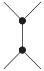
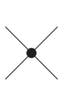
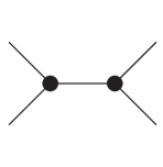
Figure 11: The merge-and-split operation applied to two adjacent antichiral vertices.

The coincidence of global poles is easy to understand from the octacut pentabox diagrams in fig. 10. Each diagram is uniquely characterized by the chiralities of the three-point vertices in the pentagon loop. Overlapping kinematical configurations are related by an elementary merge-and-split operation SplitMove ; MergeAndSplit (see fig. 11), which manifestly preserves the locations of leading singularities. The reason is the following. In a massless three-point vertex, either chiral or antichiral spinors are collinear by momentum conservation. Accordingly, for two adjacent like-chirality vertices, four spinors of the same type must be aligned. This constraint is obviously invariant under the merge-and-split operation, and therefore the cut solution is left unchanged.

This operation teaches us that octacut solutions coincide pairwise, leaving only 10 distinct global poles. As an example, we can consider the octacut diagrams that correspond to the global poles ${\cal G}_{3}$ and ${\cal G}_{4}$ of $P^{**}_{3,2}(1,2,3,4,5)$ and $P^{**}_{3,2}(3,4,5,1,2)$ respectively. They are related by merging and splitting the adjacent like-chirality vertices in the four-point tree indicated by fat lines in fig. 12. They therefore coincide. We immediately conclude that the octacut poles are identical. The same holds for the parity-conjugate poles.

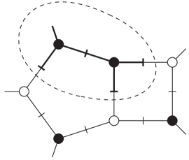
Figure 12: The octacut global poles ${\cal G}_{3}$ (left) and ${\cal G}_{2}$ (right) of respectively $P^{**}_{3,2}(\sigma_{1})$ and $P^{**}_{3,2}(\sigma_{3})$. The encircled subdiagrams are related by the split-and-merge operation.

At first glance, the sharing of global poles between different pentabox integrals would appear to preclude the use of maximal unitarity at two loops for five-point processes. It would seem to imply that we cannot isolate a specific permutation by cutting all of its eight propagators simultaneously. As was true at four points, and as we shall explain in following subsections, we can avoid this unhappy state of affairs by making use of nonhomologous contours encircling the octacut poles. Their existence ensures that the different pentabox integrals remain distinguishable, essentially through their behavior in the neighborhood of the global poles.

VIII.3 Cancellation of Octa-Cut Residues

Given that the pentabox octacut global poles coincide pairwise, it is natural to examine the implications for the corresponding residues. We shall investigate whether we can construct a sum of dual conformally invariant pentabox integrals, along with a choice of contours, that yields a vanishing residue. Such a combination would be a candidate to being expressed in terms of simpler integrals such as double boxes, factorized two-loop integrals, and products of one-loop integrals.

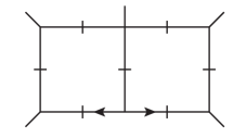
Figure 13: The two displayed permutations of the pentabox share a turtle-box heptacut. This is evident directly from the diagrams because the four-point vertex of the turtle box can be opened to a pair of three-point vertices to either loop.

Consider the following cyclic sum of pentabox integrals,

$$\sum_{\sigma\in Z_{5}}c_{\sigma}P^{**}_{3,2}[(\ell_{1}+k_{\sigma(5)}^{2}](\sigma)=\int\!\frac{d^{D}\ell_{1}}{(2\pi)^{D}}\!\int\!\frac{d^{D}\ell_{2}}{(2\pi)^{D}}$$ (88)

$$\hskip 14.22636pt\times\bigg{[}\frac{c_{\sigma_{1}}(\ell_{1}+k_{5})^{2}}{\ell_{1}^{2}(\ell_{1}-k_{1})^{2}(\ell_{1}-K_{12})^{2}(\ell_{1}-K_{123})^{2}(\ell_{1}+\ell_{2})^{2}\ell_{2}^{2}(\ell_{2}-k_{5})^{2}(\ell_{2}-K_{45})^{2}}$$

$$\hskip 14.22636pt\phantom{\times\bigg{[}}\,+\!\frac{c_{\sigma_{2}}(\ell_{1}+k_{1})^{2}}{\ell_{1}^{2}(\ell_{1}-k_{2})^{2}(\ell_{1}-K_{23})^{2}(\ell_{1}-K_{234})^{2}(\ell_{1}+\ell_{2})^{2}\ell_{2}^{2}(\ell_{2}-k_{1})^{2}(\ell_{2}-K_{51})^{2}}$$

$$\hskip 14.22636pt\phantom{\times\bigg{[}}\,+\!\!\frac{c_{\sigma_{3}}(\ell_{1}+k_{2})^{2}}{\ell_{1}^{2}(\ell_{1}-k_{3})^{2}(\ell_{1}-K_{34})^{2}(\ell_{1}-K_{345})^{2}(\ell_{1}+\ell_{2})^{2}\ell_{2}^{2}(\ell_{2}-k_{2})^{2}(\ell_{2}-K_{12})^{2}}$$

$$\hskip 14.22636pt\phantom{\times\bigg{[}}\,+\!\frac{c_{\sigma_{4}}(\ell_{1}+k_{3})^{2}}{\ell_{1}^{2}(\ell_{1}-k_{4})^{2}(\ell_{1}-K_{45})^{2}(\ell_{1}-K_{451})^{2}(\ell_{1}+\ell_{2})^{2}\ell_{2}^{2}(\ell_{2}-k_{3})^{2}(\ell_{2}-K_{23})^{2}}$$

$$\hskip 14.22636pt\phantom{\times\bigg{[}}\,+\!\frac{c_{\sigma_{5}}(\ell_{1}+k_{4})^{2}}{\ell_{1}^{2}(\ell_{1}-k_{5})^{2}(\ell_{1}-K_{51})^{2}(\ell_{1}-K_{512})^{2}(\ell_{1}+\ell_{2})^{2}\ell_{2}^{2}(\ell_{2}-k_{4})^{2}(\ell_{2}-K_{34})^{2}}\bigg{]}\,,$$

with five free parameters $c_{\sigma}$. The sum in eq. (88) runs over the cyclic permutations of the five external momenta,

$$\sigma_{1}\equiv(1,2,3,4,5)\;, \sigma_{2}\equiv(2,3,4,5,1)\;, \sigma_{3}\equiv(3,4,5,1,2)\;,$$ (89)

$$\sigma_{4}\equiv(4,5,1,2,3)\;, \sigma_{5}\equiv(5,1,2,3,4)\;.$$

We analyze each octacut global pole individually. In order to sketch the general features of the calculation, let us focus on the octacut ${\cal G}_{3}$ of the pentabox integral $P^{**}_{3,2}(\sigma_{1})$. (${\cal G}_{4}$ is then given by parity conjugation.) As explained above, this particular global pole is also present in $P^{**}_{3,2}(\sigma_{3})$ (see fig. 12). We can reparametrize the latter integral defined in the third line of eq. (88) by replacing $\ell_{2}\to-\ell_{1}-K_{345}$ and $\ell_{2}\to-\ell_{1}+K_{12}$ and thereby align seven out of the eight internal lines in a physically meaningful way,

$$c_{\sigma_{1}}P^{**}_{3,2}[(\ell_{1}+k_{5})^{2}](\sigma_{1})+c_{\sigma_{3}}P^{**}_{3,2}[(\ell_{2}+k_{1})^{2}](\sigma_{3})=$$ (90)

$$\hskip 42.67912pt\int\frac{d^{D}\ell_{1}}{(2\pi)^{D}}\int\frac{d^{D}\ell_{2}}{(2\pi)^{D}}\frac{1}{\ell_{1}^{2}(\ell_{1}-k_{1})^{2}(\ell_{1}-K_{12})^{2}(\ell_{1}+\ell_{2})^{2}(\ell_{2}-k_{5})^{2}(\ell_{2}-K_{45})^{2}}$$

$$\hskip 142.26378pt\;\;\times\bigg{(}c_{\sigma_{1}}\frac{(\ell_{1}+k_{5})^{2}}{(\ell_{1}-K_{123})^{2}}+c_{\sigma_{3}}\frac{(\ell_{2}+k_{1})^{2}}{(\ell_{2}-K_{345})^{2}}\bigg{)}\;.$$

Indeed, the two pentaboxes now naturally share a turtle-box heptacut as illustrated in fig. 13. The heptacut has six solutions, just like the heptacut of the double-box integral. Two of the solutions do not contain a pentabox octacut pole; each of the remaining solutions contains one of the global poles ${\cal G}_{1},\ldots,{\cal G}_{4}$. The turtle-box heptacut solution containing ${\cal G}_{3}$ has the form

$${\cal S}_{3}:\,\left\{\begin{array}[]{ll}\alpha_{3}=z\,,&\;\;\;\beta_{3}=0\,,\\[5.69054pt] \alpha_{4}=0\,,&\;\;\;\beta_{4}=\beta_{4}(z)\,,\end{array}\right.$$ (91)

where,

$$\beta_{4}(z)\equiv\frac{Q_{2}(P^{\bullet}_{3}-P^{\bullet}_{2})(z-P^{\bullet}_{1})}{(P^{\bullet}_{1}-P^{\bullet}_{2})(z-P^{\bullet}_{3})}\,.$$ (92)

and where $\alpha_{1,2}$ and $\beta_{1,2}$ are given by eq. (84). (The octacut pole of the pentaboxes is at $z=P^{\bullet}_{2}$, at which point $\beta_{4}$ becomes $Q_{2}$.) The Jacobians associated with the changes of variables $\ell_{1}^{\mu}\to\alpha_{i}$ and $\ell_{2}^{\mu}\to\beta_{i}$ are

$$J_{L}=\det_{\mu,i}\frac{\partial\ell_{1}^{\mu}}{\partial\alpha_{i}}=-is_{12}^{2}/4\,,\quad J_{R}=\det_{\mu,i}\frac{\partial\ell_{2}^{\mu}}{\partial\beta_{i}}=-is_{45}^{2}/4\,.$$ (93)

On this heptacut,

$$\big{(}P^{**}_{3,2}[(\ell_{1}+k_{5})^{2}](\sigma_{1})+P^{**}_{3,2}[(\ell_{2}+k_{1})^{2}](\sigma_{3})\big{)}\big{|}_{7\text{-cut}}=$$ (94)

$$\qquad\quad-\frac{1}{16s_{12}s_{45}\langle 1\,5\rangle[5\,2]}\oint\frac{dz}{z(z-P^{\bullet}_{1})}\bigg{(}c_{\sigma_{1}}\frac{(\ell_{1}+k_{5})^{2}}{(\ell_{1}-K_{123})^{2}}+c_{\sigma_{3}}\frac{(\ell_{2}+k_{1})^{2}}{(\ell_{2}-K_{345})^{2}}\bigg{)}\bigg{|}_{{\cal S}_{3}}\,.$$

We can now evaluate the terms in parentheses; denoting the sum $\Xi(z)$ for instance,

$$\Xi(\ell_{1},\ell_{2})\equiv c_{\sigma_{1}}\frac{(\ell_{1}+k_{5})^{2}}{(\ell_{1}-K_{123})^{2}}+c_{\sigma_{3}}\frac{(\ell_{2}+k_{1})^{2}}{(\ell_{2}-K_{345})^{2}}\;.$$ (95)

By direct calculation,

$$\Xi(z)|_{{\cal S}_{3}}={} -c_{\sigma_{1}}\frac{\langle 1\,5\rangle[5\,2](z-P_{1}^{\bullet})}{\langle 1\,3\rangle[3\,2](z-P_{2}^{\bullet})}-c_{\sigma_{3}}\frac{\langle 5\,1\rangle[1\,4](\beta_{4}(z)-Q_{1})}{\langle 5\,3\rangle[3\,4](\beta_{4}(z)-Q_{2})}\;.$$ (96)

At this stage it is not entirely clear how similar the terms in $\Xi$ are. The first term has a pole at $z=P^{\bullet}_{2}$; it turns out that the second term also has a pole there,

$$\mathop{\rm Res}_{z=P^{\bullet}_{2}}\frac{1}{\beta_{4}(z)-Q_{2}}={} \frac{(P^{\bullet}_{1}-P^{\bullet}_{2})(P^{\bullet}_{3}-P^{\bullet}_{2})}{(P^{\bullet}_{1}-P^{\bullet}_{3})Q_{2}}\;,$$ (97)

showing that the two pentaboxes indeed share the octacut global pole as anticipated. We combine the two terms in eq. (96) on a common denominator and take the octacut residue, first imposing the turtle-box heptacut, and then performing the contour integral in $z$. Remarkably, after some spinor algebra, we see that the residues at this pentabox octacut global pole cancel between the two integrals in question if $c_{\sigma_{1}}/c_{\sigma_{3}}=s_{23}/s_{34}$,

$$\mathop{\rm Res}_{z=P^{\bullet}_{2}}\Xi(z)|_{{\cal S}_{3}}=-\frac{s_{23}s_{51}}{\langle 1\,3\rangle[3\,2]}\frac{P^{\bullet}_{1}-P^{\bullet}_{2}}{P^{\bullet}_{1}}\left(\frac{c_{\sigma_{1}}}{s_{23}}-\frac{c_{\sigma_{3}}}{s_{34}}\right)\;.$$ (98)

We may fix the overall normalization so that the octacut residues are independent of external kinematics. For the choice $c_{\sigma_{1}}=s_{12}s_{23}s_{45}$ and $c_{\sigma_{3}}=s_{12}s_{34}s_{45}$ it follows that $\Xi|_{{\cal S}_{3}}=s_{12}s_{45}s_{51}$, so that,

$$\big{(}s_{12}s_{23}s_{45}P^{**}_{3,2}[(\ell_{1}\mskip-1.0mu\mskip-1.0mu+\mskip-1.0mu\mskip-1.0muk_{5})^{2}](\sigma_{1}) \mskip-1.0mu+\mskip-1.0mus_{34}s_{45}s_{12}P^{**}_{3,2}[(\ell_{2}\mskip-1.0mu\mskip-1.0mu+\mskip-1.0mu\mskip-1.0muk_{1})^{2}](\sigma_{3})\big{)}\big{|}_{7\text{-cut}}=\frac{P^{\bullet}_{1}}{16}\!\oint\!\frac{dz}{z(z\mskip-1.0mu\mskip-1.0mu-\mskip-1.0mu\mskip-1.0muP^{\bullet}_{1})}\,.$$ (99)

The cancellation of the pole is of course equivalent to the statement that for this choice of contour, the octacut residues are equal in magnitude, but opposite in sign.

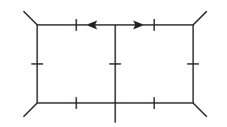
Figure 14: There is a second turtle-box heptacut which also receives contributions from two cyclic permutations of the pentabox. The dashed lines in the left and right diagrams indicate numerator insertions of $(\ell_{1}+k_{4})^{2}$ and $(\ell_{2}+k_{3})^{2}$ respectively.

What happens with the corresponding residues evaluated at the octacut global poles ${\cal G}_{1}$ and ${\cal G}_{2}$ of $P^{**}_{3,2}(\sigma_{1})$? Referring to figs. 10 and 15, we can easily guess the answer from symmetry. With an appropriate choice of contour, these residues will cancel between $P^{**}_{3,2}(\sigma_{1})$ and the cyclic permutation $P^{**}_{3,2}(\sigma_{4})$. From symmetry considerations, one possible contour corresponds to the heptacut of the turtle box shown in fig. 14, followed by a contour integral over the remaining degree of freedom. We can show this by direct computation as before. First rewrite the loop momenta in the expression for $P^{**}_{3,2}(\sigma_{1})$ in eq. (88) through the substitutions $\ell_{1}\to-\ell_{1}+K_{123}$ and $\ell_{2}\to-\ell_{2}+K_{45}$; and the expression for $P^{**}_{3,2}(\sigma_{4})$ via $\ell_{1}\to-\ell_{2}+K_{145}$ and $\ell_{2}\to-\ell_{1}+K_{23}$. The corresponding terms in eq. (88) then take the form,

$$c_{\sigma_{1}}P^{**}_{3,2}[(\ell_{1}+k_{4})^{2})](\sigma_{1})+c_{\sigma_{4}}P^{**}_{3,2}[(\ell_{2}+k_{3})^{2})](\sigma_{4})=$$ (100)

$$\hskip 42.67912pt\int\frac{d^{D}\ell_{1}}{(2\pi)^{D}}\int\frac{d^{D}\ell_{2}}{(2\pi)^{D}}\frac{1}{\ell_{1}^{2}(\ell_{1}-k_{3})^{2}(\ell_{1}-K_{23})^{2}(\ell_{1}+\ell_{2})^{2}(\ell_{2}-k_{4})^{2}(\ell_{2}-K_{45})^{2}}$$

$$\hskip 142.26378pt\;\;\times\bigg{(}c_{\sigma_{1}}\frac{(\ell_{1}+k_{4})^{2}}{(\ell_{1}-K_{123})^{2}}+c_{\sigma_{4}}\frac{(\ell_{2}+k_{3})^{2}}{(\ell_{2}-K_{451})^{2}}\bigg{)}\;.$$

It is convenient to introduce a modified loop momentum parametrization, suggested by the fact that on the heptacut, $\ell_{1}$ and $\ell_{2}$ now end up being collinear with $k_{3}$ and $k_{4}$ respectively,

$$\ell_{1}^{\mu}={} \tilde{\alpha}_{1}k_{2}^{\mu}+\tilde{\alpha}_{2}k_{3}^{\mu}+\frac{\tilde{\alpha}_{3}}{2}\left\langle 2\>\!|\>\!\sigma^{\mu}\>\!|\>\!3\right]+\frac{\tilde{\alpha}_{4}}{2}\left\langle 3\>\!|\>\!\sigma^{\mu}\>\!|\>\!2\right]\,,$$ (101)

$$\ell_{2}^{\mu}={} \tilde{\beta}_{1}k_{4}^{\mu}+\tilde{\beta}_{2}k_{5}^{\mu}+\frac{\tilde{\beta}_{3}}{2}\left\langle 4\>\!|\>\!\sigma^{\mu}\>\!|\>\!5\right]+\frac{\tilde{\beta}_{4}}{2}\left\langle 5\>\!|\>\!\sigma^{\mu}\>\!|\>\!4\right]\,.$$

Correspondingly, we also define a new set of complex values,

$$\widetilde{P}_{1}\equiv{} -\frac{\langle 3\,4\rangle}{\langle 2\,4\rangle}\,, \widetilde{P}_{2}\equiv{} \frac{[1\,2]}{[1\,3]}\,, \widetilde{P}_{3}\equiv{} -\frac{\langle 3\,5\rangle}{\langle 2\,5\rangle}\,,$$

$$\widetilde{Q}_{1}\equiv{} -\frac{[3\,4]}{[3\,5]}\,, \widetilde{Q}_{2}\equiv{} \frac{\langle 1\,5\rangle}{\langle 1\,4\rangle}\,,$$ (102)

and their parity conjugates,

$$\widetilde{P}^{\bullet}_{1}\equiv{} -\frac{[3\,4]}{[2\,4]}\;, \widetilde{P}^{\bullet}_{2}\equiv{} \frac{\langle 1\,2\rangle}{\langle 1\,3\rangle}\;, \widetilde{P}^{\bullet}_{3}\equiv{} -\frac{[3\,5]}{[2\,5]}\;,$$

$$\widetilde{Q}^{\bullet}_{1}\equiv{} -\frac{\langle 3\,4\rangle}{\langle 3\,5\rangle}\;, \widetilde{Q}^{\bullet}_{2}\equiv{} \frac{[1\,5]}{[1\,4]}\;.$$ (103)

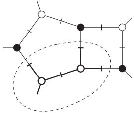
Figure 15: The octacut global poles ${\cal G}_{1}$ and ${\cal G}_{2}$ in $P^{**}_{3,2}(\sigma_{1})$ are shared with $P^{**}_{3,2}(\sigma_{4})$. As the poles are related by parity conjugation, only diagrams relevant for ${\cal G}_{1}$ are shown. The four-point subdiagram which is responsible for the sharing is marked by thicker lines and surrounded by a dashed circle.

Using these definitions, the heptacut depicted in fig. 15 is realized by fixing the loop-momentum parameters as follows,

$$\widetilde{{\cal S}}_{1}:\,\left\{\begin{array}[]{ll}\tilde{\alpha}_{3}=0\,,&\;\;\;\tilde{\alpha}_{4}=z\,,\\[5.69054pt] \tilde{\beta}_{3}=\widetilde{\beta}_{3}(z)\,,&\;\;\;\tilde{\beta}_{4}=0\,,\end{array}\right.\qquad\tilde{\beta}_{3}(z)=\frac{\widetilde{Q}_{2}(\widetilde{P}^{\bullet}_{2}-\widetilde{P}^{\bullet}_{3})(z-\widetilde{P}^{\bullet}_{1})}{(\widetilde{P}^{\bullet}_{2}-\widetilde{P}^{\bullet}_{1})(z-\widetilde{P}^{\bullet}_{3})}\;,$$ (106)

with $\tilde{\alpha}_{1}=\tilde{\beta}_{2}=0$ and $\tilde{\alpha}_{2}=\tilde{\beta}_{1}=1$. The Jacobians associated with the changes of variables $\ell_{1}^{\mu}\to\tilde{\alpha}_{i}$ and $\ell_{2}^{\mu}\to\tilde{\beta}_{i}$ are

$$\widetilde{J}_{L}=\det_{\mu,i}\frac{\partial\ell_{1}^{\mu}}{\partial\tilde{\alpha}_{i}}=-is_{23}^{2}/4\,,\quad\widetilde{J}_{R}=\det_{\mu,i}\frac{\partial\ell_{2}^{\mu}}{\partial\tilde{\beta}_{i}}=-is_{45}^{2}/4\,.$$ (107)

We can now cut the seven shared propagators to obtain,

$$\big{(}P^{**}_{3,2}[(\ell_{1}+k_{4})^{2}](\sigma_{1})+P^{**}_{3,2}[(\ell_{2}+k_{3})^{2}](\sigma_{4})\big{)}\big{|}_{7\text{-cut}}=$$ (108)

$$\hskip 42.67912pt\frac{1}{16s_{23}s_{45}\langle 3\,4\rangle[4\,2]}\oint\frac{dz}{z(z-\widetilde{P}_{1}^{\bullet})}\bigg{(}c_{\sigma_{1}}\frac{(\ell_{1}+k_{4})^{2}}{(\ell_{1}-K_{123})^{2}}+c_{\sigma_{4}}\frac{(\ell_{2}+k_{3})^{2}}{(\ell_{2}-K_{451})^{2}}\bigg{)}\bigg{|}_{\widetilde{{\cal S}}_{1}}\;.$$

As with the earlier combination (95), the terms in parentheses combine to a constant, $\big{(}\cdots\big{)}\big{|}_{\widetilde{{\cal S}}_{1}}=s_{34}$, provided that $c_{\sigma_{1}}/c_{\sigma_{4}}=s_{12}/s_{51}$. With a judicious choice of normalization we obtain,

$$\big{(}s_{12}s_{23}s_{45}P^{**}_{3,2}[(\ell_{1}\mskip-1.0mu\mskip-1.0mu+\mskip-1.0mu\mskip-1.0muk_{4})^{2}](\sigma_{1})\mskip-1.0mu+ s_{23}s_{45}s_{51}P^{**}_{3,2}[(\ell_{2}\mskip-1.0mu\mskip-1.0mu+\mskip-1.0mu\mskip-1.0muk_{3})^{2}](\sigma_{4})\big{)}\big{|}_{7\text{-cut}}=\frac{\widetilde{P}^{\bullet}_{1}}{16}\!\oint\!\frac{dz}{z(z\mskip-1.0mu\mskip-1.0mu-\mskip-1.0mu\mskip-1.0mu\widetilde{P}^{\bullet}_{1})}\,,$$ (109)

so that the pentabox octacut pole again drops out. In fact, because the relevant global poles ${\cal G}_{1,2}$ are shared by the earlier turtlebox shown in fig. 13, we could also have used that heptacut, followed by the $z$ contour integral, to demonstrate this cancellation between residues of $P^{**}_{3,2}(\sigma_{1})$ and those of $P^{**}_{3,2}(\sigma_{4})$.

In summary, of the four octacut poles of $P^{**}_{3,2}(\sigma_{1})$, the residues at the poles ${\cal G}_{3,4}$ cancel against two residues at global poles of $P^{**}_{3,2}(\sigma_{3})$, while the residues at the poles ${\cal G}_{1,2}$ cancel against two residues at global poles of $P^{**}_{3,2}(\sigma_{4})$. The pattern of cancellations extends straightforwardly to the remaining cyclically permuted dual-conformal pentabox integrals and their octacut residues. We conclude that in the cyclic sum of dual-conformal pentaboxes, the octacut realized as a turtle-box heptacut followed by a cut of the last propagator produces vanishing octacut residues because of pairwise cancellations,

$$\sum_{\rho\in\text{cyclic}}s_{12}s_{23}s_{45}P^{**}_{3,2}[(\ell_{1}+k_{\rho(5)})](\rho)\big{|}_{8\text{-cut}}=0\,.$$ (110)

This type of contour explains how the relation (76) can express a sum of pentaboxes in terms of simpler integrals, as the one-mass double boxes do not admit these particular octacuts. (Some, though not all, of the squared one-loop box integral terms admit these global poles.) The sharing of global poles which makes this possible is highly nontrivial.

VIII.4 Bowtie-Based Octa-Cuts

In the previous subsection, we saw by direct calculation that the linear combination of pentaboxes on the left-hand side of the five-point ABDK relation evaluates to zero on one combination of pentabox octacut contours. The combination is made up of contours realized as turtle-box heptacuts followed by a choice of contour for the remaining degree of freedom that puts the eighth propagator on shell.

In this subsection, we examine a different octacut contour which also has a transparent physical interpretation. It corresponds to taking the hexacut of a one-mass bow-tie integral, followed by localizing the integrand onto poles in the remaining degrees of freedom. The latter step can be thought of as opening the two four-point vertices to pairs of on-shell three-point vertices, or as probing the limit where both loop momenta become soft or collinear with an external leg. In contrast to the contours discussed in the previous subsection, each contour in the bow-tie class yields a nonvanishing residue only for one pentabox out of the five with different cyclic orderings of the external-momentum arguments.

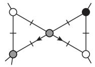
Figure 16: The one-mass bow-tie hexacut, which has two pairs of parity conjugate branches. This figure only shows branches that are not related to each other by parity conjugation. All internal lines are on-shell.

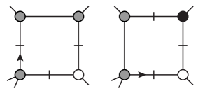
Figure 17: Products of one-loop one-mass box integrals which can support a pentabox octacut. A one-mass box with a massive corner $K_{12}$ is identified with the standard ordering $(12345)$, in agreement with the conventions for the two-loop integrals. The figure shows a particular branch of the hexacut.

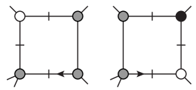
Figure 18: Products of one-loop one-mass box integrals which cannot support a pentabox octacut (since the propagator $(\ell_{1}-k_{1})$ is absent), but may contribute to double-box octacuts, i.e. residues from Jacobian poles. The figure shows a particular configuration of chiral, antichiral and nonchiral vertices.

Consider the one-mass bow-tie hexacut with the standard ordering of the external legs and standard labeling of loop momenta, shown in fig. 16. One pentabox integral along with one one-mass double-box integral share this hexacut. What other integrals can share it? As we are interested in analyzing a cross-order integral relation, we are led to consider products of one-loop integrals. There is an obvious candidate to share this cut: a product of one-mass box integrals. If we examine the right-side loop in either of the diagrams in fig. 16, we see that we can complete the three propagators to a one-loop box in one of two ways, with the massive leg carrying either $K_{12}$ or $K_{23}$. We can complete the three propagators on the left-side loop in two ways as well, with the massive leg carrying either $K_{45}$ or $K_{12}$. Overall, this leaves us with four possible combinations of one-mass boxes, which are shown in figs. 17 and 18. We have chosen the loop-momentum labelings in order to align six of the eight internal lines between the pentabox and the products of one-loop integrals in a physical way. This gives us the following expressions,

$$I_{\square}(\sigma_{4})\times I_{\square}(\sigma_{1})\equiv{} \int\frac{d^{D}\ell_{1}}{(2\pi)^{D}}\frac{1}{\ell_{1}^{2}(\ell_{1}-k_{1})^{2}(\ell_{1}-K_{12})^{2}(\ell_{1}-K_{123})^{2}}$$

$$\qquad\quad\times\int\frac{d^{D}\ell_{2}}{(2\pi)^{D}}\frac{1}{\ell_{2}^{2}(\ell_{2}-k_{5})^{2}(\ell_{2}-K_{45})^{2}(\ell_{2}-K_{345})^{2}}\,,$$ (111)

$$I_{\square}(\sigma_{4})\times I_{\square}(\sigma_{2})\equiv{} \int\frac{d^{D}\ell_{1}}{(2\pi)^{D}}\frac{1}{\ell_{1}^{2}(\ell_{1}-k_{1})^{2}(\ell_{1}-K_{12})^{2}(\ell_{1}-K_{123})^{2}}$$

$$\qquad\quad\times\int\frac{d^{D}\ell_{2}}{(2\pi)^{D}}\frac{1}{\ell_{2}^{2}(\ell_{2}-k_{5})^{2}(\ell_{2}-K_{45})^{2}(\ell_{2}+k_{1})^{2}}\,,$$ (112)

$$I_{\square}(\sigma_{1})\times I_{\square}(\sigma_{1})\equiv{} \int\frac{d^{D}\ell_{1}}{(2\pi)^{D}}\frac{1}{\ell_{1}^{2}(\ell_{1}-K_{12})^{2}(\ell_{1}-K_{123})^{2}(\ell_{1}+k_{5})^{2}}$$

$$\qquad\quad\times\int\frac{d^{D}\ell_{2}}{(2\pi)^{d}}\frac{1}{\ell_{2}^{2}(\ell_{2}-k_{5})^{2}(\ell_{2}-K_{45})^{2}(\ell_{2}-K_{345})^{2}}\,,$$ (113)

$$I_{\square}(\sigma_{1})\times I_{\square}(\sigma_{2})\equiv{} \int\frac{d^{D}\ell_{1}}{(2\pi)^{D}}\frac{1}{\ell_{1}^{2}(\ell_{1}-K_{12})^{2}(\ell_{1}-K_{123})^{2}(\ell_{1}+k_{5})^{2}}$$

$$\qquad\quad\times\int\frac{d^{D}\ell_{2}}{(2\pi)^{D}}\frac{1}{\ell_{2}^{2}(\ell_{2}-k_{5})^{2}(\ell_{2}-K_{45})^{2}(\ell_{2}+k_{1})^{2}}\,.$$ (114)

In these equations, the $\sigma_{i}$ refer to the orderings given in eq. (89), with the massive leg made up of the first two arguments as in eq. (78).

The hexacut shown in fig. 16 defines the two-dimensional algebraic variety,

$${\cal S}\equiv\big{\{}\,(\ell_{1},\ell_{2})\in{\mathbb{C}\mathbb{P}}^{4}\times{\mathbb{C}\mathbb{P}}^{4}\;\big{|} \ell_{1}^{2}=0\,,\;(\ell_{1}-K_{12})^{2}=0\,,\;(\ell_{1}-K_{123})^{2}=0\,,\;$$ (115)

$$\ell_{2}^{2}=0\,,\;(\ell_{2}-k_{5})^{2}=0\,,\;(\ell_{2}-K_{45})^{2}=0\,\big{\}}\;.$$

As in the four-point case there are four classes of hexacut solutions, each parametrized by two complex variables $(z_{1},z_{2})\in\mathbb{C}^{2}$. By parity, it is sufficient to consider the cuts depicted in fig. 16. Here we focus mainly on the kinematics of the first of the two cuts, see fig. 19.

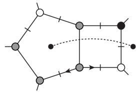
Figure 19: The one-mass bow-tie hexacut embeds several genuine two-loop integrals. Our basis includes the dual conformal pentabox and the one-mass double box. The figure shows a particular kinematical configuration.

As in the four-point case with the massless bow-tie integral (60), the one-mass bow-tie hexacut is just a product of independent cuts of one-loop triangle integrals. This makes it straightforward to write down solutions. The natural loop-momentum parametrization for this problem is

$$\ell_{1}^{\mu}={} \hat{\alpha}_{1}K_{12}^{\flat,\mu}+\hat{\alpha}_{2}k_{3}^{\mu}-\frac{\hat{\alpha}_{3}\langle 1\,K_{12}^{\flat}\rangle}{2\,\langle 2\,3\rangle}\left\langle k_{3}\>\!|\>\!\sigma^{\mu}\>\!|\>\!K_{12}^{\flat}\right]-\frac{\hat{\alpha}_{4}[1\,K_{12}^{\flat}]}{2\,[2\,3]}\left\langle K_{12}^{\flat}\>\!|\>\!\sigma^{\mu}\>\!|\>\!k_{3}\right]\;,$$ (116)

$$\ell_{2}^{\mu}={} \beta_{1}k_{4}^{\mu}+\beta_{2}k_{5}^{\mu}+\frac{\beta_{3}}{2}\left\langle k_{4}\>\!|\>\!\sigma^{\mu}\>\!|\>\!k_{5}\right]+\frac{\beta_{4}}{2}\left\langle k_{5}\>\!|\>\!\sigma^{\mu}\>\!|\>\!k_{4}\right]\;,$$

where the flattened vector $K_{12}^{\flat}$ (projected along the direction of momentum $k_{3}$) is defined by,

$$K_{12}^{\flat,\mu}\equiv{} K_{12}^{\mu}-\frac{K_{12}^{2}}{\gamma_{1}}k_{3}^{\mu}\;.$$ (117)

In this equation, $\gamma_{1}\equiv 2K_{12}\cdot k_{3}$. We can then write down the solutions to the hexacut equations. All solutions share the following parameter values,

$$\hat{\alpha}_{1}=1\,,\;\;\hat{\alpha}_{2}=0\,,\;\;\beta_{1}=0\,,\;\;\beta_{2}=1\,.$$ (118)

The solution ${\cal S}_{1}$ corresponding to the left diagram in fig. 16 is given by the following values of the remaining parameters,

$$\hat{\alpha}_{3}=0\,,\;\;\hat{\alpha}_{4}=z_{1}\,,\;\;\beta_{3}=z_{2}\,,\;\;\beta_{4}=0\,.$$ (119)

The parity-conjugate solution ${\cal S}_{2}$ is given by,

$$\hat{\alpha}_{3}=z_{1}\,,\;\;\hat{\alpha}_{4}=0\,,\;\;\beta_{3}=0\,,\;\;\beta_{4}=z_{2}\,.$$ (120)

The solution ${\cal S}_{3}$ corresponding to the right diagram in fig. 16 is given by,

$$\hat{\alpha}_{3}=0\,,\;\;\hat{\alpha}_{4}=z_{1}\,,\;\;\beta_{3}=0\,,\;\;\beta_{4}=z_{2}\,.$$ (121)

The last solution ${\cal S}_{4}$ is the parity-conjugate to ${\cal S}_{3}$, and is given by,

$$\hat{\alpha}_{3}=z_{1}\,,\;\;\hat{\alpha}_{4}=0\,,\;\;\beta_{3}=z_{2}\,,\;\;\beta_{4}=0\,.$$ (122)

The bow-tie hexacut one-mass double-box and pentabox integrals are,

$$P^{**}_{2,2}[1](\sigma_{1})\big{|}_{6\text{-cut}}={} \oint_{\widetilde{\Gamma}}d^{2}z\frac{J_{\bowtie}^{-1}(z_{1},z_{2})}{(\ell_{1}+\ell_{2})^{2}}\bigg{|}_{{\cal S}_{i}}\;,$$ (123)

$$P^{**}_{3,2}[(\ell_{1}+k_{5})^{2}](\sigma_{1})\big{|}_{6\text{-cut}}={} \oint_{\widetilde{\Gamma}}d^{2}z\frac{J_{\bowtie}^{-1}(z_{1},z_{2})(\ell_{1}+k_{5})^{2}}{(\ell_{1}-k_{1})^{2}(\ell_{1}+\ell_{2})^{2}}\bigg{|}_{{\cal S}_{i}}\,,$$

and similarly for the products of one-mass boxes. In these equations, $J_{\bowtie}^{-1}(z_{1},z_{2})$ is the net inverse Jacobian from performing the hexacut (including the Jacobians from the change of variables from the loop momenta to the parameters $\hat{\alpha}_{i}$ and $\beta_{i}$). It has the same value for all solutions,

$$J_{\bowtie}^{-1}(z_{1},z_{2})\equiv-\frac{1}{16\gamma_{1}s_{45}}\frac{1}{z_{1}z_{2}}\;.$$ (124)

The contour $\widetilde{\Gamma}$ is in general a weighted sum of contours surrounding global poles within the four solutions.

For the most general treatment, parity-odd terms such as the pentagon on the one-loop side and Levi-Civita numerators that integrate to zero must be included as well. Here we instead construct linear combinations of residues in order to project out parity-odd terms from the integrands on both sides of the ABDK relation (76). On the two-loop side, it suffices to take parity-even contours that encircle two parity-conjugate global poles with the same weight. Both factors in a product of one-loop one-mass boxes with a Levi-Civita insertion in either loop also integrate to zero, although the product of Levi-Civita contractions is really a Gram determinant. Accordingly, in general we have to encircle at least four global poles to produce a consistent contour. It is easy to show that the poles must be two parity-conjugate pairs which are in turn related by parity-conjugation of either the left or right loop. This leads us to consider sums over the four solutions,

$$P^{**}_{2,2}[1](\sigma_{1})\big{|}_{6\text{-cut}}={} \sum_{i=1}^{4}\oint_{\widetilde{\Gamma}_{i}}c_{i}^{(\Gamma)}d^{2}z\frac{J_{\bowtie}^{-1}(z_{1},z_{2})}{(\ell_{1}+\ell_{2})^{2}}\bigg{|}_{{\cal S}_{i}}\;,$$ (125)

$$P^{**}_{3,2}[(\ell_{1}+k_{5})^{2}](\sigma_{1})\big{|}_{6\text{-cut}}={} \sum_{i=1}^{4}\oint_{\widetilde{\Gamma}_{i}}c_{i}^{(\Gamma)}d^{2}z\frac{J_{\bowtie}^{-1}(z_{1},z_{2})(\ell_{1}+k_{5})^{2}}{(\ell_{1}-k_{1})^{2}(\ell_{1}+\ell_{2})^{2}}\bigg{|}_{{\cal S}_{i}}\,,$$

where $\widetilde{\Gamma}_{i}$ is the image in ${\cal S}_{i}$ of a given contour in ${\cal S}_{1}$ under the parity conjugation, under the parity operation on the right-side loop, or under the combined operation. We will choose different sets of global poles, and corresponding contours, to isolate different terms. (In this analysis, there will be a unique contour enclosing each global pole.) The coefficients $c_{i}^{(\Gamma)}$ will be chosen in order to enforce the absence of parity-odd terms on the right-hand side. These coefficients could in principle be different for different global poles. Some of the global poles will be shared between different solutions ${\cal S}_{i}$; we must be careful to take only one copy of such global poles in the sum.

We determined the coefficients of the dual-conformal pentabox integrals in the previous subsection. We are left with the task of determining the one-mass double-box and squared one-loop one-mass box coefficients in the relation. We start with the hexacut,

$$\sum_{i=1}^{4}c_{i}^{(\Gamma)}\oint_{\widetilde{\Gamma}_{i}}d^{2}z\,J_{\bowtie}^{-1}(z_{1},z_{2})\bigg{[}\frac{c_{\sigma_{1}}(\ell_{1}+k_{5})^{2}}{(\ell_{1}-k_{1})^{2}(\ell_{1}+\ell_{2})^{2}}+\frac{c_{1\text{m},\sigma_{1}}}{(\ell_{1}+\ell_{2})^{2}}\bigg{]}\bigg{|}_{{\cal S}_{i}}=$$ (126)

$$\hskip 36.98857pt\sum_{i=1}^{4}c_{i}^{(\Gamma)}\oint_{\widetilde{\Gamma}_{i}}d^{2}z\,J_{\bowtie}^{-1}(z_{1},z_{2})\bigg{[} \frac{c_{\sigma_{4}\times\sigma_{1}}}{(\ell_{1}-k_{1})^{2}(\ell_{2}-K_{345})^{2}}+\frac{c_{\sigma_{4}\times\sigma_{2}}}{(\ell_{1}-k_{1})^{2}(\ell_{2}+k_{1})^{2}}$$

$$+\frac{c_{\sigma_{1}\times\sigma_{1}}}{(\ell_{1}+k_{5})^{2}(\ell_{2}-K_{345})^{2}}+\frac{c_{\sigma_{1}\times\sigma_{2}}}{(\ell_{1}+k_{5})^{2}(\ell_{2}+k_{1})^{2}}\bigg{]}\bigg{|}_{{\cal S}_{i}}\,.$$

and re-express it in terms of the unfixed variables on the different solutions. The solution ${\cal S}_{1}$ gives the following contribution to the equation,

$$c_{i}^{(\Gamma)} \oint_{\widetilde{\Gamma}_{1}}d^{2}z\,\frac{1}{16s_{45}z_{1}z_{2}}\biggl{[} \!\frac{c_{\sigma_{1}}P_{2}Q^{\bullet}_{2}}{s_{12}s_{23}(z_{1}\!-\!P_{2})(z_{2}\!-\!Q^{\bullet}_{2})}\!-\!\frac{c_{1\text{m},\sigma_{1}}[2\,3]}{\langle 2\,3\rangle\langle 4\,5\rangle[1\,2][3\,5]^{2}(z_{1}\!-\!P_{4})(z_{2}\!-\!Q^{\bullet}_{2})}\biggr{]}\overset{\Sigma}{=}$$ (127)

$$\hskip 28.45274ptc_{i}^{(\Gamma)}\oint_{\widetilde{\Gamma}_{1}}d^{2}z\;\frac{1}{16s_{45}z_{1}z_{2}}\biggl{[} \frac{c_{\sigma_{4}\times\sigma_{1}}}{s_{12}\langle 2\,3\rangle[1\,3]\langle 3\,4\rangle[3\,5](z_{1}\!-\!P_{2})(z_{2}\!-\!Q^{\bullet}_{2})}$$

$$-\frac{c_{\sigma_{4}\times\sigma_{2}}}{s_{12}[1\,3]\langle 1\,4\rangle\langle 2\,3\rangle[1\,5](z_{1}\!-\!P_{2})(z_{2}\!-\!Q^{\bullet}_{1})}$$

$$-\frac{c_{\sigma_{1}\times\sigma_{1}}[2\,3]}{s_{34}\langle 2\,3\rangle\langle 4\,5\rangle[1\,2][3\,5]^{2}(z_{1}\!-\!P_{4})(z_{2}\!-\!Q^{\bullet}_{2})}$$

$$-\frac{c_{\sigma_{1}\times\sigma_{2}}[2\,3]}{\langle 1\,4\rangle\langle 2\,3\rangle\langle 4\,5\rangle[1\,2][1\,5][3\,4][3\,5](z_{1}\!-\!P_{4})(z_{2}\!-\!Q^{\bullet}_{1})}\biggr{]}\,.$$

where the notation ‘$\overset{\Sigma}{=}$’ means that the equality holds only after summing over all four solutions. In this expression, we have introduced labels for two additional complex values and their parity conjugates,

$$P_{4}\equiv\frac{\langle 3\,4\rangle[2\,3][4\,5]}{\langle 2\,3\rangle[1\,2][3\,5]}\,,\qquad P^{\bullet}_{4}\equiv\frac{[3\,4]\langle 2\,3\rangle\langle 4\,5\rangle}{[2\,3]\langle 1\,2\rangle\langle 3\,5\rangle}\,.$$ (128)

From solution ${\cal S}_{2}$, we obtain the spinor conjugate of eq. (127). From solution ${\cal S}_{3}$, we obtain,

$$-c_{i}^{(\Gamma)}\oint_{\widetilde{\Gamma}_{3}}\frac{d^{2}z}{16s_{45}z_{1}z_{2}}$$ (129)

$$\hskip 14.22636pt\times\biggl{[}-\frac{c_{\sigma_{1}}[3\,5](z_{1}\!-\!P_{4})}{\langle 1\,2\rangle(z_{1}\!-\!P_{2})\big{(}\langle 2\,3\rangle[1\,2][1\,3][3\,4](z_{1}\!-\!P_{2})(z_{2}\!+\!{Q^{\bullet}_{2}}{}^{-1})\!+\!\gamma_{1}[1\,4][2\,3](z_{2}\!-\!Q_{1})\big{)}}$$

$$\hskip 14.22636pt\hphantom{\times\biggl{[}}\;+\frac{c_{1\text{m},\sigma_{1}}[2\,3][1\,3]}{\langle 4\,5\rangle[3\,4]\big{(}\langle 2\,3\rangle[1\,2][1\,3][3\,4](z_{1}\!-\!P_{2})(z_{2}\!+\!Q^{\bullet}_{2}{}^{-1})\!+\!\gamma_{1}[1\,4][2\,3](z_{2}\!-\!Q_{1})\big{)}}\biggr{]}\overset{\Sigma}{=}$$

$$\hskip 28.45274pt-c_{i}^{(\Gamma)}\oint_{\widetilde{\Gamma}_{3}}\frac{d^{2}z}{16s_{45}z_{1}z_{2}}\biggl{[} \frac{c_{\sigma_{4}\times\sigma_{1}}}{s_{12}\langle 2\,3\rangle\langle 3\,5\rangle[1\,3][3\,4](z_{1}\!-\!P_{2})(z_{2}\!-\!Q_{2})}$$

$$-\frac{c_{\sigma_{4}\times\sigma_{2}}}{s_{12}\langle 2\,3\rangle\langle 1\,5\rangle[1\,3][1\,4](z_{1}\!-\!P_{2})(z_{2}\!-\!Q_{1})}$$

$$-\frac{c_{\sigma_{1}\times\sigma_{1}}[2\,3]}{s_{35}\langle 2\,3\rangle\langle 4\,5\rangle[1\,2][3\,4]^{2}(z_{1}\!-\!P_{4})(z_{2}\!-\!Q_{2})}$$

$$-\frac{c_{\sigma_{1}\times\sigma_{2}}[2\,3]}{\langle 2\,3\rangle\langle 4\,5\rangle[1\,2][3\,4][1\,4][3\,5]\langle 1\,5\rangle(z_{1}\!-\!P_{4})(z_{2}\!-\!Q_{1})}\biggr{]}\,.$$

From solution ${\cal S}_{4}$, we obtain the spinor conjugate of this equation. The minus signs on both sides of eq. (129) arise from the relative ordering of the six variables we integrate in order to obtain this form, compared to the canonical order,

$$d\hat{\alpha}_{1}\wedge d\hat{\alpha}_{2}\wedge d\hat{\alpha}_{3}\wedge d\hat{\alpha}_{4}\wedge d\beta_{1}\wedge d\beta_{2}\wedge d\beta_{3}\wedge d\beta_{4}\,;$$ (130)

in eq. (127), we must permute one variable ($\beta_{4}$) twice to the left, whereas in eq. (129), we must permute one variable ($\beta_{3}$) once to the left. One might be tempted to cancel the minus signs on both sides of eq. (129), but that would alter the relative signs between different solutions.

Most of the singularities in eqs. (127) and (129) are manifest; in order to see what singularities may arise from the more intricate denominators on the left-hand side of eq. (129), consider two limits,

$$\big{(}\langle 2\,3\rangle[1\,2][1\,3][3\,4] (z_{1}\!-\!P_{2})(z_{2}\!+\!{Q^{\bullet}_{2}}{}^{-1})\!+\!\gamma_{1}[1\,4][2\,3](z_{2}\!-\!Q_{1})\big{)}\big{|}_{z_{1}=0}=$$ (131)

$$\langle 3\,5\rangle[1\,3][2\,3][4\,5](z_{2}-Q_{2})\,,$$

$$\big{(}\langle 2\,3\rangle[1\,2][1\,3][3\,4] (z_{1}\!-\!P_{2})(z_{2}\!+\!{Q^{\bullet}_{2}}{}^{-1})\!+\!\gamma_{1}[1\,4][2\,3](z_{2}\!-\!Q_{1})\big{)}\big{|}_{z_{2}=0}=$$

$$\langle 2\,3\rangle[1\,2][1\,3][3\,5](z_{1}-P_{4})\,.$$

Thus, taking the residue at $z_{1}=0$ will reveal a pole at $z_{2}=Q_{2}$; and taking the residue at $z_{2}=0$ will reveal a pole at $z_{1}=P_{4}$.

We can now enumerate the global poles. Sixteen poles are located within the bulk of a single solution; we can group these into four sets, where the poles in each set are related by parity and the right-loop parity operation, with $(z_{1},z_{2})$ values,

$$\textrm{I}: \quad(P_{2},Q^{\bullet}_{2});\quad(P^{\bullet}_{2},Q_{2});\quad(P_{2},Q_{2});\quad(P^{\bullet}_{2},Q^{\bullet}_{2});$$ (132)

$$\textrm{II}: \quad(P_{2},Q^{\bullet}_{1});\quad(P^{\bullet}_{2},Q_{1});\quad(P_{2},Q_{1});\quad(P^{\bullet}_{2},Q^{\bullet}_{1});$$

$$\textrm{III}: \quad(P_{4},Q^{\bullet}_{2});\quad(P^{\bullet}_{4},Q_{2});\quad(P_{4},Q_{2});\quad(P^{\bullet}_{4},Q^{\bullet}_{2});$$

$$\textrm{IV}: \quad(P_{4},Q^{\bullet}_{1});\quad(P^{\bullet}_{4},Q_{1});\quad(P_{4},Q_{1});\quad(P^{\bullet}_{4},Q^{\bullet}_{1}).$$

The sum in eq. (125) is over the global poles within each of these sets. We will determine the appropriate coefficients below. The last set has residues only for the one-loop box squared terms; as in the four-point case in Sec. VII, we do not consider them.

Six poles are each shared between two solutions; we can group these into three pairs

$$\textrm{V}: \quad(P_{2},0);\quad(P^{\bullet}_{2},0);$$ (133)

$$\textrm{VI}: \quad(P_{4},0);\quad(P^{\bullet}_{4},0);$$

$$\textrm{VII}: \quad(0,Q^{\bullet}_{2});\quad(0,Q_{2}).$$

The first pole in the first two pairs is shared between solutions ${\cal S}_{1}$ and ${\cal S}_{3}$, and the second is shared between solutions ${\cal S}_{2}$ and ${\cal S}_{4}$. In the last pair, the first pole is shared between ${\cal S}_{1}$ and ${\cal S}_{4}$, and the second between ${\cal S}_{2}$ and ${\cal S}_{3}$. We can avoid double counting by picking the poles out of ${\cal S}_{1,2}$ in all three cases, setting $c^{(\Gamma)}_{3,4}=0$.

Finally, one global pole, at $(z_{1},z_{2})=(0,0)$, is shared between all four solutions. We can avoid overcounting the pole by setting $c^{(\Gamma)}_{2,3,4}=0$.

In the one-loop box squared terms, there are three distinct numerators that give rise to vanishing integrals: an insertion of a parity-odd numerator in either integral, or a simultaneous insertion in both. These are the integrals which the sum in eq. (125) is intended to eliminate. For the first set in eq. (132), for example, we have the following constraints,

$$\sum_{i=1}^{4}c_{i}^{(\Gamma)}\oint_{\widetilde{\Gamma}_{i}}d^{2}z\,J_{\bowtie}^{-1}(z_{1},z_{2})\frac{\varepsilon(\ell_{1},k_{1},k_{2},k_{3})}{(\ell_{1}-k_{1})^{2}(\ell_{2}-K_{345})^{2}}=0\,,$$ (134)

$$\sum_{i=1}^{4}c_{i}^{(\Gamma)}\oint_{\widetilde{\Gamma}_{i}}d^{2}z\,J_{\bowtie}^{-1}(z_{1},z_{2})\frac{\varepsilon(\ell_{2},k_{3},k_{4},k_{5})}{(\ell_{1}-k_{1})^{2}(\ell_{2}-K_{345})^{2}}=0\,,$$

$$\sum_{i=1}^{4}c_{i}^{(\Gamma)}\oint_{\widetilde{\Gamma}_{i}}d^{2}z\,J_{\bowtie}^{-1}(z_{1},z_{2})\frac{\varepsilon(\ell_{1},k_{1},k_{2},k_{3})\varepsilon(\ell_{2},k_{3},k_{4},k_{5})}{(\ell_{1}-k_{1})^{2}(\ell_{2}-K_{345})^{2}}=0\,.$$

Evaluating the integrands on the various solutions (and omitting overall $z_{i}$-independent factors), these equations become,

$$0 =-c_{1}^{(\Gamma)}\oint_{\widetilde{\Gamma}_{1}}\!d^{2}z\,\frac{1}{\langle 3\,4\rangle[3\,5]z_{2}(z_{1}\!-\!P_{2})(z_{2}\!-\!Q^{\bullet}_{2})}+c_{2}^{(\Gamma)}\oint_{\widetilde{\Gamma}_{2}}\!d^{2}z\,\frac{1}{\langle 3\,5\rangle[3\,4]z_{2}(z_{1}\!-\!P^{\bullet}_{2})(z_{2}\!-\!Q_{2})}$$ (135)

$$+c_{3}^{(\Gamma)}\oint_{\widetilde{\Gamma}_{3}}\!d^{2}z\,\frac{1}{\langle 3\,5\rangle[3\,4]z_{2}(z_{1}\!-\!P_{2})(z_{2}\!-\!Q_{2})}-c_{4}^{(\Gamma)}\oint_{\widetilde{\Gamma}_{4}}\!d^{2}z\,\frac{1}{\langle 3\,4\rangle[3\,5]z_{2}(z_{1}\!-\!P^{\bullet}_{2})(z_{2}\!-\!Q^{\bullet}_{2})}\,,$$

$$0 =c_{1}^{(\Gamma)}\!\oint_{\widetilde{\Gamma}_{1}}\!d^{2}z\,\frac{1}{\langle 2\,3\rangle[1\,3]z_{1}(z_{1}\!-\!P_{2})(z_{2}\!-\!Q^{\bullet}_{2})}$$

$$\hskip 14.22636pt-c_{2}^{(\Gamma)}\!\oint_{\widetilde{\Gamma}_{2}}\!d^{2}z\,\frac{1}{\langle 1\,3\rangle[2\,3]z_{1}(z_{1}\!-\!P^{\bullet}_{2})(z_{2}\!-\!Q_{2})}$$

$$\hskip 14.22636pt+c_{3}^{(\Gamma)}\!\oint_{\widetilde{\Gamma}_{3}}\!d^{2}z\,\frac{1}{\langle 2\,3\rangle[1\,3]z_{1}(z_{1}\!-\!P_{2})(z_{2}\!-\!Q_{2})}$$

$$\hskip 14.22636pt-c_{4}^{(\Gamma)}\!\oint_{\widetilde{\Gamma}_{4}}d^{2}z\,\ \frac{1}{\langle 1\,3\rangle[2\,3]z_{1}(z_{1}\!-\!P^{\bullet}_{2})(z_{2}\!-\!Q^{\bullet}_{2})}\,,$$

$$0 =-c_{1}^{(\Gamma)}\oint_{\widetilde{\Gamma}_{1}}\!d^{2}z\,\frac{1}{(z_{1}\!-\!P_{2})(z_{2}\!-\!Q^{\bullet}_{2})}-c_{2}^{(\Gamma)}\oint_{\widetilde{\Gamma}_{2}}\!d^{2}z\,\frac{1}{(z_{1}\!-\!P^{\bullet}_{2})(z_{2}\!-\!Q_{2})}$$

$$-c_{3}^{(\Gamma)}\oint_{\widetilde{\Gamma}_{3}}\!d^{2}z\,\frac{1}{(z_{1}\!-\!P_{2})(z_{2}\!-\!Q_{2})}-c_{4}^{(\Gamma)}\oint_{\widetilde{\Gamma}_{4}}d^{2}z\,\ \frac{1}{(z_{1}-P^{\bullet}_{2})(z_{2}-Q^{\bullet}_{2})}\,.$$

Evaluating the residues on set I of the poles in eq. (132), we find the equations,

$$0 =\frac{1}{s_{34}}\bigl{(}c_{1}^{(\Gamma)}-c_{2}^{(\Gamma)}-c_{3}^{(\Gamma)}+c_{4}^{(\Gamma)}\bigr{)}\,,$$ (136)

$$0 =-\frac{1}{s_{23}}\bigl{(}c_{1}^{(\Gamma)}-c_{2}^{(\Gamma)}+c_{3}^{(\Gamma)}-c_{4}^{(\Gamma)}\bigr{)}\,,$$

$$0 =-\bigl{(}c_{1}^{(\Gamma)}+c_{2}^{(\Gamma)}+c_{3}^{(\Gamma)}+c_{4}^{(\Gamma)}\bigr{)}\,.$$

Solving these equations, we find,

$$c_{2}^{(\Gamma)}=c_{1}^{(\Gamma)},\quad c_{3}^{(\Gamma)}=-c_{1}^{(\Gamma)},\quad c_{4}^{(\Gamma)}=-c_{1}^{(\Gamma)}.$$ (137)

The solution is the same for the other pole sets in eq. (132). For the pairs in eq. (133), we find,

$$c_{2}^{(\Gamma)}=c_{1}^{(\Gamma)}.$$ (138)

The pole sets in eqs. (132) and (133) are shared between the left- and right-hand sides of eq. (125). With the coefficients $c_{i}^{(\Gamma)}$ determined, we can obtain equations for the coefficients of the various integrals by matching sums of residues at the different pole sets. From set I, we obtain,

$$c_{\sigma_{4}\times\sigma_{1}}={\textstyle\frac{1}{2}}s_{34}c_{\sigma_{1}}\,;$$ (139)

using the value chosen for $c_{\sigma_{1}}$ in the previous subsection, we find,

$$c_{\sigma_{4}\times\sigma_{1}}={\textstyle\frac{1}{2}}s_{12}s_{23}s_{34}s_{45}\,.$$ (140)

From set II, we obtain,

$$c_{\sigma_{4}\times\sigma_{2}}={\textstyle\frac{1}{2}}s_{51}c_{\sigma_{1}}={\textstyle\frac{1}{2}}s_{12}s_{23}s_{45}s_{51}\,.$$ (141)

From set III, we obtain a relation between $c_{\sigma_{1}\times\sigma_{1}}$ and $c_{1\text{m},\sigma_{1}}$,

$$c_{\sigma_{1}\times\sigma_{1}}={\textstyle\frac{1}{2}}s_{34}c_{1\text{m},\sigma_{1}}\,.$$ (142)

As noted above, the set IV consists of poles that appear only in the one-loop box squared terms, and as in the four-point case, we set these aside. The pair V gives no new information beyond eqs. (139) and (141). From the pair VI, after substituting eq. (142), we obtain a relation for $c_{\sigma_{1}\times\sigma_{2}}$,

$$c_{\sigma_{1}\times\sigma_{2}}={\textstyle\frac{1}{2}}s_{51}c_{1\text{m},\sigma_{1}}\,.$$ (143)

From the pair VII, we obtain a solution for $c_{1\text{m},\sigma_{1}}$ after substituting eqs. (139) and (142),

$$c_{1\text{m},\sigma_{1}}=\frac{s_{34}s_{45}}{s_{12}s_{23}}c_{\sigma_{1}}=s_{34}s_{45}^{2}\,.$$ (144)

With this value, we also find,

$$c_{\sigma_{1}\times\sigma_{1}} ={\textstyle\frac{1}{2}}s_{34}^{2}s_{45}^{2}\,,$$ (145)

$$c_{\sigma_{1}\times\sigma_{2}} ={\textstyle\frac{1}{2}}s_{34}s_{45}^{2}s_{51}\,.$$

The remaining pole, at $(z_{1},z_{2})=(0,0)$, gives no additional equations.

As in the four-point case, the integrands of the squared one-loop box terms are symmetric under the interchange $\ell_{1}\leftrightarrow\ell_{2}$, whereas the integrands of the pentaboxes and one-mass double boxes are not. This means that in symmetrizing the integrands following the discussion at the end of Sec. VII, the left-hand side’s residues will acquire an extra factor of $1/2$. The same will also be true of the product of non-identical one-loop boxes, because the residue extraction above will find non-vanishing residues only for one of the two terms. Accordingly, the factors of $1/8$ noted at the beginning of this section for the pentaboxes and one-mass double boxes will become $1/16$, whereas the one-loop box squared terms and the product of different one-loop boxes will have factors of $1/32$ in front of their residues. The relative factor of $1/2$ is precisely what is seen above in eqs. (139–145).

The matching of residues thus leads precisely to the integral coefficients present in the five-point ABDK relation (76). In other words, we have reconstructed the parity-even leading-localization part of the ABDK relation in the maximally supersymmetric Yang–Mills theory. We will not discuss the details, but we have also checked explicitly that an analysis of the hexacut, including all parity-even and -odd contributions, yields a residue-by-residue match of the leading-localization terms in the relation, without the need for summing over sets of residues as in the discussion above.

IX Discussion and Conclusions

In this paper, we have studied the two-loop ABDK/BDS relation from the viewpoint of maximal generalized unitarity. The coefficients of integrals in an amplitude in this approach are given by multivariate contour integrals of products of trees. The multivariate contour integrals are taken around global poles, and unlike the single-variable case, there can be several non-homologous contours surrounding a given global pole. We gave a simple example of this in Sec. II.2. Different integrals can share a global pole, but in some instances have different residues with respect to different contours surrounding the pole.

It turns out that the left- and right-hand sides of the ABDK relation (2) and (76) do indeed share global poles, and have residues with respect to a common contour. This allows us to match contributions on both sides of the relation for the global poles of the planar two-loop integrals. The matches allow us to determine the coefficients of the one-loop box squared terms on the right-hand side of eqs. (2) and (76), and of the pentabox on the left-hand side of eq. (76). We leave to future work puzzles associated with residues appearing only on the right-hand side, not shared by planar two-loop integrals. In addition, the right-hand sides also have terms not detectable in the maximal localizations of the integrals that we perform, such the one-loop amplitude in $D=4-4\epsilon$ dimensions. It would be interesting to see if these are also accessible to generalized-unitarity techniques. The analysis in this paper suggests that maximal generalized-unitarity techniques can be used to search for new integral or amplitude identities beyond the ones dictated by dual conformal invariance.