Improving M-SBL for Joint Sparse Recovery using a Subspace Penalty
Abstract
The multiple measurement vector problem (MMV) is a generalization of the compressed sensing problem that addresses the recovery of a set of jointly sparse signal vectors. One of the important contributions of this paper is to reveal that the seemingly least related state-of-art MMV joint sparse recovery algorithms - M-SBL (multiple sparse Bayesian learning) and subspace-based hybrid greedy algorithms - have a very important link. More specifically, we show that replacing the term in M-SBL by a rank proxy that exploits the spark reduction property discovered in subspace-based joint sparse recovery algorithms, provides significant improvements. In particular, if we use the Schatten- quasi-norm as the corresponding rank proxy, the global minimiser of the proposed algorithm becomes identical to the true solution as . Furthermore, under the same regularity conditions, we show that the convergence to a local minimiser is guaranteed using an alternating minimization algorithm that has closed form expressions for each of the minimization steps, which are convex. Numerical simulations under a variety of scenarios in terms of SNR, and condition number of the signal amplitude matrix demonstrate that the proposed algorithm consistently outperforms M-SBL and other state-of-the art algorithms.
Index Terms:
Compressed sensing, joint sparse recovery, multiple measurement vector problem, subspace method, M-SBL, generalized MUSIC criterion, rank proxy, Schatten- normCorrespondence to:
Jong Chul Ye, Ph.D. Professor
Dept. of Bio and Brain Engineering, KAIST
291 Daehak-ro Yuseong-gu, Daejon 305-701, Republic of Korea
Email: jong.ye@kaist.ac.kr
Tel: 82-42-350-4320
Fax: 82-42-350-4310
I Introduction
The multiple measurement vector problem (MMV) is a generalization of the compressed sensing problem, which addresses the recovery of a set of sparse signal vectors that share a common support [1, 2, 3, 4, 5, 6]. In the MMV model, let and denote the number of sensor elements and snapshots, respectively; and denote the length of the signal vectors. Then, for a given noisy observation matrix and a sensing matrix , the multiple measurement vector (MMV) problem can be formulated as:
| (1) | |||
where is the -th signal, , is the -th row of , and , where is the set of indices of nonzero rows in . The Frobenius norm is used to measure the discrepancy between the data and the model. Classically, pursuit algorithms such as alternating minimization algorithm (AM) and MUSIC (multiple signal classification) algorithm [7], S-OMP (simultaneous orthogonal matching pursuit) [8, 2], M-FOCUSS [3], randomized algorithms such as REduce MMV and BOost (ReMBo)[4], and model-based compressive sensing using block-sparsity [9, 10] have been applied to the MMV problem.
An algebraic bound for the recoverable sparisity level has been theoretically studied by Feng and Bresler [7], and by Chen and Huo [2] for noiseless measurement . More specifically, if satisfies and
| (2) |
where denotes the smallest number of linearly dependent columns of , then is the unique solution of (1). This indicates that the recoverable sparsity level may increase with an increasing number of measurement vectors. Indeed, for noiseless measurement, a MUSIC algorithm by Feng and Bresler [7] is shown to achieve the performance limit when the measurement matrix is full rank. However, except for MUSIC in full rank cases, the performance of the aforementioned classical MMV algorithms is not generally satisfactory, falling far short of (2) even for the noiseless case, when only a finite number of snapshots are available.
In a noisy environment, Obozinski et al showed that a near optimal sampling rate reduction up to can be achieved using mixed norm penalty [11]. A similar gain was observed in computationally inexpensive greedy approaches such as compressive MUSIC (CS-MUSIC) [1] and subspace augmented MUSIC (SA-MUSIC) [6]. More specifically, Kim et al [1] and Lee et al [6] independently showed that a class of hybrid greedy algorithms that combine greedy steps with a so called generalized MUSIC subspace criterion [1], or equivalently, with subspace augmentation [6], can reduce the required number of measurements by up to in noisy environment. Furthermore, using a large system MMV model, Kim et al further showed that for an i.i.d. Gaussian sensing matrix, their algorithm can asymptotically achieve the algebraic performance limit when increases with a particular scaling law [1]. Lee et al [6] also showed that MUSIC can do this in the noisy case and full rank, non-asymptotically with finite data, and for realistic Fourier sensing matrices.
While the aforementioned mixed norm approach and subspace based greedy approaches provide theoretical performance guarantees, there also exist a very different class of powerful MMV algorithms that are based on empirical Bayesian and Automatic Relevance Determination (ARD) principles from machine learning. Among these, the so-called multiple sparse Bayesian learning (M-SBL) algorithm is best known [12]. Even though M-SBL is more computationally expensive than greedy algorithms such as CS-MUSIC or SA-MUSIC, empirical results show that M-SBL is quite robust to noise and to unfavorable restricted isometry property constant (RIC) of the sensing matrix [13]. Moreover, M-SBL is more competitive than mixed norm approaches. Since Bayesian approaches are very different from classical compressed sensing, such high performance appears mysterious at first glance. However, a recent breakthrough by Wipf et al unveiled that M-SBL can be converted to a standard compressed sensing framework with an additional (log determinant) penalty - a non-separable sparsity inducing prior [14]. The presence of the non-separable penalty term is so powerful that M-SBL performs almost as well as MUSIC. However, the guarantee only applies to the full row rank case of with noise-free measurement vectors [15, 12]. However, despite its excellent performance, compared to the mixed norm approaches or subspace greedy algorithms, other than the work by Wipf et al [14], the fundamental theoretical analysis of M-SBL has been limited.
Therefore, one of the main goals of this paper is to continue the effort by Wipf et al [14] and analyze the origin of the high performance of M-SBL, as well as to investigate its limitations. One of the important contributions of this paper is to show that the seemingly least related algorithms - M-SBL and subspace-based hybrid greedy algorithms - have a very important link. More specifically, we show that the term in M-SBL is a proxy for the rank of a partial sensing matrix corresponding to the true support. We then show that minimising the rank that was discovered in subspace-based hybrid greedy algorithm to exploit the spark reduction property of MMV can indeed provide a true solution for the MMV problem. Accordingly, replacing term in M-SBL by a Schatten- quasi-norm rank proxy provides significant performance improvements.
The resulting new algorithm is no longer Bayesian due to the use of a deterministic penalty based on a geometric argument, so we call the new algorithm subspace-penalized sparse learning (SPL) by excluding term “Bayesian”. We show that as in the Schatten -norm rank proxy, the global minimizers of the SPL cost function are identical to those of the original minimization problem. Furthermore, we show that SPL can be easily implemented as an alternating minimization approach.
Using numerical simulations, we demonstrate that compared to the current state-of-art MMV algorithms such as mixed norm approaches, M-SBL, CS-MUSIC/SA-MUSIC, and sequential CS-MUSIC [13], SPL provides superior recovery performance. Moreover, the results show that SPL is very robust to noise, and to the condition number of the unknown signal matrix.
I-A Notation
Throughout the paper, and correspond to the -th row and the -th column of matrix , respectively. The element of is represented by . When is an index set, , and correspond to a submatrix collecting corresponding rows of and columns of , respectively. For a matrix , is the trace of a matrix , is its adjoint, denotes the Penrose-Moor psuedo-inverse, refers the determinant, denotes the range space of , and (or ) and (or ) are the projection on the range space and its orthogonal complement, respectively. The vector denotes an elementary unit vector whose -th element is 1, and denotes an identity matrix.
A sensing matrix is said to have a -restricted isometry property (RIP) if there exist left and right RIP constants such that
for all such that . A single RIP constant is often referred to as the RIP constant.
II M-SBL: A Review
II-A Algorithm Description
Under appropriate assumptions of noise and signal Gaussian statistics, one can show that M-SBL minimizes the following cost function in a so-called space [12]:
| (3) |
where
| , | (4) |
With an estimate of , which typically has a nearly sparse diagonal and may be thresholded to be exactly sparse, the solution of M-SBL is given by
| (5) |
One of the most important contributions by Wipf is that the minimization problem of the cost function (3) can be equivalently represented as the following standard sparse recovery framework [14]:
| (6) |
where is a penalty given by
| (7) |
where
| (8) |
Wipf et al [14] gave a heuristic argument showing that corresponds to a non-separable sparsity promoting penalty, and proposed the following alternating minimization approach to solve the minimization problem (6).
II-A1 Step 1: Minimization with respect to
For a given estimate at the -th iteration, we can find a closed form solution for in (6):
For large scale problems, this can be computed using a standard conjugate gradient algorithm with an appropriate preconditioner.
II-A2 Step 2: Minimization with respect to
In this step, for a given we need to solve the following minimization problem:
where
| (9) |
Wipf et al [14] find the solution to . More specifically, the derivative with respect to each component is given by
| (10) |
since
Setting the derivative to zero after fixing , this observation leads to the following fixed point update of :
| (11) |
II-B Role of the Non-separable Penalty in M-SBL
In order to develop a new joint sparse recovery algorithm that improves on M-SBL, we provide here a new interpretation of the role of the regularization term in M-SBL. Note that due to the non-negativity constraint for , a critical solution to the minimization problem in (7) should satisfy the following first order Karush-Kuhn-Tucker (KKT) necessary conditions [16]:
Hence, as , this leads to the following fixed point equation:
If , using the matrix inversion lemma, we have
| (12) | |||||
where denotes a nonzero support of and denotes the orthogonal projection on the span of the columns of indexed by . Accordingly,
Therefore, we have
| (13) |
Substituting (13) into (7) yields
| (14) | |||||
Note that the first term in (14) imposes row sparsity on since for due to (13). Hence, the first term of M-SBL penalty is in fact . Then, what is the meaning of the term ? Wipf et al [14] showed that the superior performance of the M-SBL is owing to the non-separability of the term with respect to , which can avoid many local minimizers. In addition to this interpretation, the following section shows another important geometric implications of the term.
III Subspace-Penalized Sparse Learning
III-A Key Observation
In this section, we provide another interpretation of the M-SBL penalty, which suggests a new algorithm called subspace-penalized sparse learning (SPL) that overcomes the limitation of M-SBL. Note that for any matrix with , we have
| (15) |
where denote the singular values of . Therefore, the function is a concave proxy for nonzero singular values, hence in the limit of , (15) acts as a proxy for [17, 18]. This leads us to another interpretation: the penalty term in M-SBL is equivalent to
| (16) |
where dentoes a rank proxy. Thus, the penalty simultaneously imposes the row sparsity of as well as the low rank of the matrix . By inspection, the first sparsity penalty term in (16) is quite intuitive, but it is not clear why needs to be minimized.
In fact, the main contribution of this paper is that we need to replace the second term, , by geometrically more intuitive rank proxy as follows:
| (17) |
where denotes a basis for the noise subspace denoted as . In the following, we will describe in detail how we arrive at the new rank penalty.
III-B Subspace Criteria
A solution for that satisfies is called a basic feasible solution (BFS) [14]. Among BFSs, a solution of the following MMV problem is called maximally sparse solution:
| , | (18) |
To address (18), subspace-based greedy algorithms such as CS-MUSIC [1] and SA-MUSIC [6] exploit the spark reduction principle or or an equivalent subspace criterion using an augmented signal subspace. More specifically, if and denotes the number of the non-zero rows, the algorithms first estimate partial support index , then the remaining components of the support are found using the subspace criterion.
One of the main contributions of this paper is that this two step approach is not necessary. Instead, for noiseless measurements, a direct minimization of the rank of with respect to index , , still guarantees to obtain the true support as shown in Theorem III.1. We believe that this is an extremely powerful result that provides an important clue to overcome the limitation of existing greedy subspace methods [1, 6] .
Theorem III.1
Assume that , , satisfy , where , and the columns of are linearly independent. If satisfies a RIP condition , then we have
and
Proof:
Since is a nondecreasing function of , we may consider . By the rank-nullity Theorem, for with . Furthermore, because ,
| (19) |
and because , by the RIP condition . Since , we have so that
| (20) |
which also implies that for any . Hence, denoting , it is enough to show that
| (21) |
and
| (22) |
First we will show that (21) holds. Because and , we have that or . Also, since by (19), we have . Hence . On the other hand, by (20), the dimension of is at most , which implies
, so that we have
Then, (22) is the only a remaining part to prove. Suppose that we have an index set such that and Then, it
must hold that
It follows that . Then, for each column of , so that there exists such that . Then, so that there is a such that with .
Since and for any , it follows that has rank . Hence, because the row rank of a matrix equals its column rank, must have linearly independent rows. Therefore, there is a subset of such that , and the rows of are linearly independent.
Since , for every there is a nonzero vector , so that we have and , since by the linearly independence of the rows of . Since , we have .
Now, because , we have . Hence . It follows that
Hence, by the RIP of , we must have . Since , we also have , which implies that . Since can be any element in , we have for any . It implies that so that since Hence, in order to satisfy and , we must have ∎
III-C The SPL Penalty
Note that minimizing with respect to is equivalent to finding the index set that minimizes . Hence, Theorem III.1 implies that minimizing under the constraint will find that has non-zero values for indices corresponding to , where and . This observation leads to the second term in the SPL penalty of (17) as a rank proxy to exploit this geometric finding.
Moreover, rather than just using as in M-SBL, in this paper, we use more general family of rank proxies that still satisfy our goals. Specifically, our rank proxy is based on Schatten- quasi norm with that includes the popular nuclear norm as a special case. For a matrix , the Scatten -norm proxy for the rank is defined as
| (23) |
which corresponds to the nuclear norm when . Following the derivation that leads to (7), we propose the following SPL penalty:
| (24) |
where
| (25) |
Using the proposed SPL penalty, we formulate the following noiseless SPL minimization problem:
| (26) |
Note that is a concave function with respect to its singular values, so we can find its convex conjugate:
| (27) |
where is given as
| (28) |
for such that ; and denotes the set of symmetric positive semi-definite matrices:
The relationship between (28) and (25) can be clearly understood by minimizing (28) with respect to . Indeed, using and [19], we have
| (29) |
and
Here, should be understood as applying the power operation to the non-zero singular values of while retaining zero singular values at zero.
Notice that is a surrogate function that majorizes . Although like (25), (28) is not jointly convex with respect to the different variables, the reason to prefer (28) over (25) is that (28) is convex with respect to each of the variables , and with the other held constant, and we can obtain a closed-form expression in each step of alternating minimization. Specifically, recall that the SPL penalty is given by
| (30) |
where
Let denotes the non-zero support set of . Using the KKT condition with respect to , we have
| (31) | |||||
| (32) |
which leads to for , whereas for
Hence, and we have
This implies that at the KKT point, the SPL penalty has cost function values equivalent to the Schatten- quasi-norm rank penalty for .
IV The SPL Algorithm
IV-A Alternating Minimization Algorithm
So far, we have analyzed the global minimizer for the noiseless SPL algorithm. For noisy measurement, we propose the following cost function:
| (33) |
By letting , the solution of (33) becomes a solution of (26) when since then the constraint is automatically satisfied as follows:
Similar equivalence can be hold for if . Therefore, rather than dealing with Eqs. (26) and (33) separately, we use (33) and the limiting argument to discuss a noiseless SPL optimization problem.
Then, using (30), a noisy SPL formulation can be written as
| (34) |
where the augmented cost function is given by
| (35) |
While is not convex for all these variables simultaneously due to the presence of the bi-convex terms and , it is convex with respect to each variable and separately. Indeed, this is a typical example of the d.c. algorithm (DCA) for the difference of convex functions programming [20, 21], and the alternating minimization algorithm converges to a local minimizer or a critical point.
Specifically, a critical solution should satisfy the following first order Karush-Kuhn-Tucker (KKT) necessary conditions [16]:
| (36) | |||||
| (37) | |||||
| (38) | |||||
| (39) |
This leads us to the following fixed point iterations:
IV-A1 Minimization with respect to
For a given estimate , (36) yields a closed form solution for :
IV-A2 Determination of
For a given estimate , using (37), we can find a closed-form solution for : i.e.
IV-A3 Estimation of
For a given and , using Eqs. (38) and (39), we have
| (40) |
Here, if , we have the following update equation:
| (41) |
Note that the SPL updates appears similar to those of M-SBL except the update by (41), which is now modified based on subspace geometry. This is the main ingredient for the performance improvement of SPL over M-SBL. In the following, we further discuss several important properties of the SPL penalty.
IV-B Properties of the SPL Penalty
An interesting case occurs when . In this case, based on (40), we have the following two observations: 1) when ; and 2) can be an arbitrary positive number when since the equality in (40) is satisfied regardless of the choice of . Therefore, we define the following update111In a practical implementation, a tolerance around 0 and finites values for have to be used.:
| (45) |
Thanks to (45), even if becomes erroneously zero during the iterations, there is a possibility, when , for to become nonzero; hence, the corresponding row of can become nonzero once turns into nonzero. Note that this is very different from M-SBL, since in (11) the denominator term cannot be zero even under the most relaxed RIP constraint , so the condition will set the corresponding to zero. Therefore, in M-SBL, once a row of is set to zero in error, it will stay zero for all subsequent iterations and the algorithm is unable to recover from this error.
Second, it is important note that since , we have ; so
| (46) |
where denotes the index set of non-zero diagonal elements of . Hence, in this case, the SPL algorithm with is the algorithm that directly minimizes the rank of . In this case, the corresponding update rule is given by
| , | (47) |
The main technical challenge is, however, that for the cost function (35) is not well-defined. Therefore, the aforementioned interpretation of the SPL should be understood as an asymptotic result such that and approach zero, but are not exactly zero.
Next, as a by product of Theorem III.1, the SPL algorithm is computationally more efficient than M-SBL. Note that the computational bottleneck of M-SBL (or SPL) is due to the the inversion of (or , respectively). Specifically, unlike the update step that can be done using the conjugate gradient (CG) algorithm, the matrix inversion cannot be performed using CG and usually is performed using the singular value decomposition (SVD). Now, note that the size of matrix in SPL is compared to for , which reduces the cost of matrix inversion for SPL compared to M-SBL. In particular, for the case of MUSIC where and , matrix inversion is not necessary for SPL whereas M-SBL still requires the matrix inversion.
Finally, note that the hyper-parameter is closely related to spectral estimation. For example, for the case of MUSIC where and , the term in (47) reduces a scalar and we have
| (48) | |||||
| (49) |
where the first term is the MUSIC spectrum and the second term is related to the magnitude of the -th row of . Hence, in the case of full-row rank (i.e., the MUSIC case), SPL can be regarded as an algorithm that initialises he non-zero support estimation using a spectral estimation technique, followed by alternating modification using the data fidelity matching criterion.
V NUMERICAL RESULTS
In this section, we perform extensive numerical experiments to validate the proposed algorithm under various experimental conditions, and compare it with respect to existing joint sparse recovery algorithms. In particular, we are interested in the SPL algorithm in the asymptotic region of since it directly minimises the rank of .
The elements of a sensing matrix were generated from a Gaussian distribution with zero mean and variance of , and then each column of was normalized to have an unit norm. An unknown signal with was generated using the same procedure as in [6]. Specifically, we randomly generated a support , and then the corresponding nonzero signal components were obtained by
| (50) |
where was set to random orthonormal columns, and is a diagonal matrix whose -th element is given by
| (51) |
and was generated using Gaussian random distribution with zero mean and variance of . After generating noiseless data, we added zero mean white Gaussian noise. We declared success if an estimated support from a certain algorithm was the same as a true .
As the proposed algorithm does not require a prior knowledge of the sparsity level, we need to define a stoping criterion. Here, the stopping criterion is defined by monitoring the normalized change in the variable :
From our experiments, usually 20-30 iterations are required for SPL to converge.
V-A Local Minima Property
We first perform experiments to confirm that SPL produces the true solution under milder conditions than M-SBL. To show this, using -sparse signal generated by (50) with , we produced measurements such that . Then, we initialized both algorithms with that satisfies the following:
| (52) |
where , and , respectively. Note that the initialization corresponds to a local minimiser and we are interested in confirming that SPL can escape from the local minimizers thanks to the update in (45). Recall that it is difficult for M-SBL to avoid this type of local minimizers since has zeros rows at the -th row where and the M-SBL update rule in (11) cannot make the corresponding nonzero in the subsequent iterations.
Figs. 1(a)-(c) illustrate the perfect recovery ratio from the initialization using SPL and M-SBL at various SNR conditions for (a) , (b) , and (c) , respectively. The results clearly demonstrate that SPL finds the global minimizer nearly perfectly, whereas M-SBL fails most of the time. This clearly confirms the theoretical advantages for SPL.

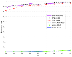
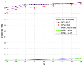
(a) (b) (c)
V-B Comparison with Other State-of-Art Algorithms
(a) (b)

(c) (d)
(e) (f)
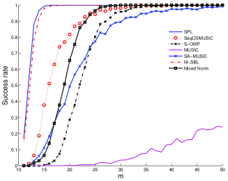
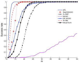
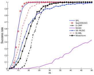
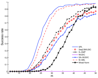
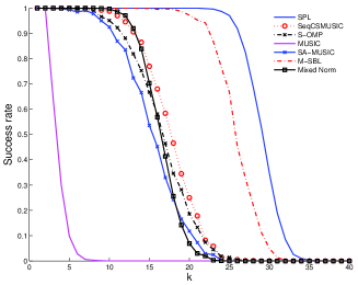
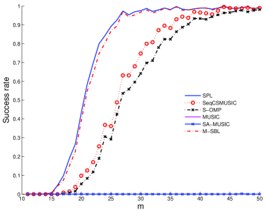
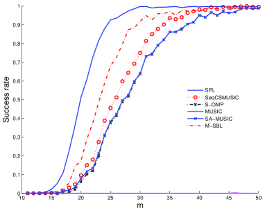
To compare the proposed algorithm with various state-of-art joint sparse recovery methods, the recovery rates of various state-of-art joint sparse recovery algorithms such as MUSIC, S-OMP, SA-MUSIC, sequential CS-MUSIC, M-SBL, and the mixed norm approach are plotted in Fig. 2 along with those of SPL. Among the various implementation of mixed norm approaches, we used high performance SGPL1 software [22], which can be downloaded from . Since M-SBL, the mixed norm approach, as well as SPL do not provide an exact -sparse solution, we used the support for the largest coefficients as a support estimate in calculating the perfect recovery ratio. For MUSIC, S-OMP, SA-MUSIC, sequential CS-MUSIC, we assume that is known. For subspace based algorithms such as MUSIC, SA-MUSIC, sequential CS-MUSIC as well as SPL, we determine the signal subspace using the following criterion
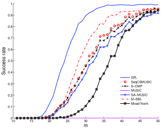
where denotes the singular values of . A theoretical motivation for such subspace determination is given in [6]. Here, the success rates were averaged over experiments. The simulation parameters were as follows: , , , and , respectively. Figs. 2(a)-(d) illustrates the comparison results under various snapshot number and SNR conditions. Note that SPL consistently outperforms all other algorithms at various snapshots numbers. In particular, the gain increases with increasing number of snapshots, since it provides better subspace estimation. Also, note that SPL consistently outperforms M-SBL at all SNR ranges. Figs. 2(e)(f) illustrates that SPL significantly outperforms M-SBL when is badly conditioned. Moreover, as the subspace estimation becomes accurate with increasing , the performance gain becomes more significant.

(a) (b) (c)
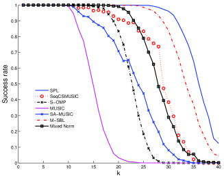
Figs. 3(a)(b)(c) compares the performance of various MMV algorithm by varying the sparsity level. Here, and are fixed and the sparsity levels changes, and we calculated the perfect reconstruction ratio. Again, SPL outperforms all existing methods for various SNR and conditions numbers.
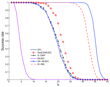
V-C Fourier Measurements Cases
Fig. 4 illustrates the results of the comparison when the measurement are from Fourier sensing matrix. Similar to Gaussian sensing matrix, consistent improvement of SPL over M-SBL and other algorithms under various conditions have been observed.
(a) (b)

(c) (d)
VI CONCLUSION
In this paper, we derived a new MMV algorithm called subspace penalized sparse learning (SPL) to address a joint sparse recovery problem, in which the unknown signals share a common non-zero support. The SPL algorithm was inspired by the observation that the term in M-SBL is a rank proxy for a partial sensing matrix, and similar rank criteria exist in subspace-based greedy MMV algorithms like CS-MUSIC and SA-MUSIC. Furthermore, we proved that instead of , minimizing is a more direct way of imposing joint sparsity since its global minimizer can provide the true joint support. To impose such a subspace constraint as a penalty, the SPL algorithm employs the Schatten- quasi norm rank penalty and was implemented as an alternating minimisation method. Theoretical analysis showed that as , the global minimizer of the SPL is equivalent to the global minimiser of the MMV solution. We further demonstrated that compared to M-SBL, our SPL is more robust to recovering badly conditioned . With numerical simulations, we demonstrated that SPL consistently outperforms all existing state-of-the art algorithms including M-SBL.
Acknowledgements
This work was supported by Korea Science and Engineering Foundation under Grant NRF-2014R1A2A1A11052491.
References
- [1] J. Kim, O. Lee, and J. Ye, “Compressive MUSIC: revisiting the link between compressive sensing and array signal processing,” IEEE Trans. on Information Theory, vol. 58, no. 1, pp. 278–301, 2012.
- [2] J. Chen and X. Huo, “Theoretical results on sparse representations of multiple measurement vectors,” IEEE Trans. on Signal Processing, vol. 54, no. 12, pp. 4634–4643, 2006.
- [3] S. Cotter, B. Rao, K. Engan, and K. Kreutz-Delgado, “Sparse solutions to linear inverse problems with multiple measurement vectors,” IEEE Trans. on Signal Processing, vol. 53, no. 7, p. 2477, 2005.
- [4] M. Mishali and Y. C. Eldar, “Reduce and boost: Recovering arbitrary sets of jointly sparse vectors,” IEEE Trans. on Signal Processing, vol. 56, pp. 4692–4702, 2009.
- [5] E. Berg and M. P. Friedlander, “Theoretical and empirical results for recovery from multiple measurements,” IEEE Trans. on Information Theory, vol. 56, no. 5, pp. 2516–2527, 2010.
- [6] K. Lee, Y. Bresler, and M. Junge, “Subspace methods for joint sparse recovery,” IEEE Trans. on Information Theory, vol. 58, no. 6, pp. 3613–3641, 2012.
- [7] P. Feng, “Universal minimum-rate sampling and spectrum-blind reconstruction for multiband signals,” Ph.D. Dissertation, University of Illinois, Urbana-Champaign, 1997.
- [8] J. Tropp, A. Gilbert, and M. Strauss, “Algorithms for simultaneous sparse approximation. Part I: Greedy pursuit,” Signal Processing, vol. 86, no. 3, pp. 572–588, 2006.
- [9] Y. Eldar, P. Kuppinger, and H. Bolcskei, “Block-sparse signals: Uncertainty relations and efficient recovery,” IEEE Trans. on Signal Processing, vol. 58, pp. 3042–3054, 2010.
- [10] R. Baraniuk, V. Cevher, M. Duarte, and C. Hegde, “Model-based compressive sensing,” IEEE Trans. on Information Theory, vol. 56, no. 4, pp. 1982–2001, 2010.
- [11] G. Obozinski, M. Wainwright, and M. Jordan, “Support union recovery in high-dimensional multivariate regression,” The Annals of Statistics, vol. 39, no. 1, pp. 1–47, 2011.
- [12] D. Wipf and B. Rao, “An empirical Bayesian strategy for solving the simultaneous sparse approximation problem,” IEEE Trans. on Signal Processing, vol. 55, no. 7 Part 2, pp. 3704–3716, 2007.
- [13] J. M. Kim, O. K. Lee, and J. C. Ye, “Improving noise robustness in subspace-based joint sparse recovery,” IEEE Trans. on Signal Processing (in press), 2012.
- [14] D. Wipf, B. Rao, and S. Nagarajan, “Latent variable bayesian models for promoting sparsity,” IEEE Trans. on Information Theory, vol. 57, no. 9, p. 6236, 2011.
- [15] D. Wipf, “Bayesian methods for finding sparse representations,” Ph.D. dissertation, University of California, San Diego, 2006.
- [16] E. K. P. Chong and S. H. Zak, An Introduction to Optimization. New York: Wiley-Interscience, 1996.
- [17] K. Mohan and M. Fazel, “Iterative reweighted least squares for matrix rank minimization,” in 48th IEEE Annual Allerton Conference on Communication, Control, and Computing, 2010, pp. 653–661.
- [18] M. Fazel, H. Hindi, and S. Boyd, “Log-det heuristic for matrix rank minimization with applications to hankel and euclidean distance matrices,” in American Control Conference, 2003. Proceedings of the 2003, vol. 3. IEEE, 2003, pp. 2156–2162.
- [19] K. Petersen and M. Pedersen, “The matrix cookbook,” Technical University of Denmark, pp. 7–15, 2008.
- [20] P. Tao and L. An, “Convex analysis approach to dc programming: Theory, algorithms and applications,” Acta Mathematica Vietnamica, vol. 22, no. 1, pp. 289–355, 1997.
- [21] P. Tao and L. T. H. An, “A DC optimization algorithm for solving the trust-region subproblem,” SIAM Journal on Optimization, vol. 8, no. 2, pp. 476–505, 1998.
- [22] E. Van Den Berg and M. Friedlander, “Probing the pareto frontier for basis pursuit solutions,” SIAM Journal on Scientific Computing, vol. 31, no. 2, p. 890, 2008.