Efficiency and Sensitivity Analysis of Observation Networks for Atmospheric Inverse Modelling with Emissions

Abstract

The controllability of advection-diffusion systems, subject to uncertain initial values and emission rates, is estimated, given sparse and error affected observations of prognostic state variables. In predictive geophysical model systems, like atmospheric chemistry simulations, different parameter families influence the temporal evolution of the system. This renders initial-value-only optimisation by traditional data assimilation methods as insufficient. In this paper, a quantitative assessment method on validation of measurement configurations to optimize initial values and emission rates, and how to balance them, is introduced. In this theoretical approach, Kalman filter and smoother and their ensemble based versions are combined with a singular value decomposition, to evaluate the potential improvement associated with specific observational network configurations. Further, with the same singular vector analysis for the efficiency of observations, their sensitivity to model control can be identified by determining the direction and strength of maximum perturbation in a finite-time interval.

Keywords: Atmospheric transport model, emission rate optimisation, observability, observational network configuration, singular value decomposition, data assimilation

1 Introduction

Air quality and climate change are influenced by the fluxes of green house gases, reactive gas emissions and aerosols in the atmosphere. The ability to quantify variable, yet hardly observable emission rates is a key problem to be solved for the analysis of atmospheric systems, and typically addressed by elaborate and costly field campaigns or permanently operational observation networks. The temporal evolution of chemistry in the atmosphere is usually modelled by atmospheric chemistry transport models. Optimal simulations are based on techniques of combining numerical models with observations. In meteorological forecast models, where initial values are insufficiently well known, while exerting a high influence on the model evolution, this procedure is termed data assimilation ([8]). There is no doubt that the optimization of the initial state is always of great importance for the improvement of predictive skill. However, especially for chemistry transport or greenhouse gas models with high dependence on the emissions in the troposphere, the optimization of initial state is no longer the only issue. The lack of ability to observe and estimate surface emission fluxes directly with necessary accuracy is a major roadblock, hampering the progress in predictive skills of climate and atmospheric chemistry models. In order to obtain the Best Linear Unbiased Estimation (BLUE) from the model with observations, efforts of optimization included the emission rates by spatio-temporal data assimilation have been made. The first full chemical implementation of the 4D-variational method for atmospheric chemistry initial values is introduced in [9]. Further, Elbern et al. ([11]) took the strong constraint of the diurnal profile shape of emission rates such that their amplitudes and initial values are the only uncertainty to be optimized and then implemented it by 4D-variational inversion. This strong constraint approach is reasonable because the diurnal evolution of emissions are typically much better known than the absolute amount of daily emissions. Moreover, several data assimilation strategies were designed to adjust ozone initial conditions and emission rates separately or jointly in [23]. Bocquet et al. introduced a straightforward extension of the iterative ensemble Kalman smoother in [2].

In many cases, the better estimations of both the initial state and emission rates are not always sustained based on appropriate observational network configurations when using popular data assimilation methods, such as 4D-variation and Kalman filter and smoother. It may hamper the optimization by unbalanced weights between the initial state and emission rates, which can, in practice, even result in degraded simulations beyond the time intervall with available observations. The ability to evaluate the suitability of an observational network to control chemical states and emission rates for its optimised designis the a key qualification, which needs to be adressed.

Singular value decomposition (SVD) can help identifying the priorities of observations by detecting the fastest growing uncertainties. The targeted observations problem is an important topic in the field of numerical weather prediction. Singular vector analysis based on SVD was firstly introduced to numerical weather prediction by Lorenz ([21]), who applied it to analyse the largest error growth rates in an idealised atmospheric model. Because of the high cost of computation, the singular vector analysis was not widely applied until 1980s. Later the method of singular vector analysis of states of the meteorological model with high dimension was feasible ([6]).

In atmospheric chemistry, studies about the importance of observations are still sparse. Khattatov et al. ([17]) firstly analysed the uncertainty of a chemical compositions. Liao et al. ([18]) focused on the optimal placement of observation locations of the chemical transport model. However, singular vector analysis for atmospheric chemistry with emissions is different since emissions play an similarly important role in forecast accuracy with initial values. Goris and Elbern ([14]) recently used the singular vector decomposition to determine the sensitivity of the chemical composition to emissions and initial values for a variety of chemical scenarios and integration length.

Hence, in this paper, applying the Kalman filter and smoother as the desirable data assimilation method we introduce an approach to identify the sensitivities of a network to optimize emission rates and initial values independently and balanced prior to any data assimilation procedure. Through singular value decomposition and ensemble Kalman filter and smoother, the computational cost of this approach can be reduced so that it is feasible in practice. Then, by the equivalence between 4D variation and Kalman filter for linear models, the approach is also feasible for the data assimilation of adjoint models via 4D variational techniques.

This paper is organized as follows. In section 2, we describe the atmospheric transport-diffusion model with emission rates first and then reconstruct the state vector such that the emission rates are included dynamically. In section 3, the theoretical approach derives in order to determine the efficiency of observations or observational network configurations before running any data assimilation procedure. In section 4, based on the theoretical analysis in section 3, we discuss the ensemble approach to evaluate the efficiency of observation configurations and present elementary examples. In section 5, we present the approach to identify the sensitivity of observations by determining the directions of maximum perturbation growth to the initial perturbation. In the appendices, the above approaches are generalised to continuous-time systems for comprehensive applications.

2 Model description

The chemical tendency equation including emission rates, propagating forward in time, is usually described by the following atmospheric transport model

$$\dfrac{dc}{dt}=\mathcal{A}(c)+e(t),$$

where $\mathcal{A}$ is a nonlinear model operator, $c(t)$ and $e(t)$ are the state vector of chemical constituents and emission rates at time $t$, respectively .

The a priori estimate of the state vector of concentrations $c(t)$ is given and denoted by $c_{b}(t)$, termed background state. The a priori estimate of emission rates are usually taken from emission inventories, denoted by $e_{b}(t)$.

Let $\mathbf{A}$ be the tangent linear operator of $\mathcal{A}$, the evolution of the perturbation of states $c(t)$ and $e(t)$ follows the tangent linear model with $\mathbf{A}$ as

$$\frac{d\delta c}{dt}=\mathbf{A}\delta c+\delta e(t),$$ (1)

where $\delta c(t)$ is the perturbation evolving from the perturbation of initial state of chemical state $\delta c(t_{0})=c(t_{0})-c_{b}(t_{0})$ and emission rates $\delta e(t)=e(t)-e_{b}(t)$.

After discretizing the tangent linear model in space, let $M(\cdot,\cdot)$ be the evolution operator or resolvent generated by $\mathbf{A}$. It is straightforward to obtain the linear solution of (1) with continuous time as

$$\delta c(t)=M(t,t_{0})\delta c(t_{0})+\int_{t_{0}}^{t}M(t,s)\delta e(s)ds,$$ (2)

where $\delta c(t)\in\mathds{R}^{n}$, $\delta e(t)\in\mathds{R}^{n}$, $n$ the dimension of the partial phase space of concentrations and emission rates. Obviously, $M(\cdot,\cdot)\in\mathds{R}^{n\times n}$.

In addition, let $y(t)$ be the observation configuration of $c(t)$ and define

$$\delta y(t)=y(t)-\mathcal{H}(t)c_{b}(t),$$

where $\mathcal{H}(t)$ is a nonlinear forward observation operator mapping the model space to the observation space. Then by linearising the nonlinear operator $\mathcal{H}$ as $H$, the linearised model equivalents of observation configurations can be presented as

$$\delta y(t)=H(t)\delta c(t)+\nu(t),$$

where $\delta y(t)\in\mathds{R}^{m(t)}$, $m(t)$ the dimension of the phase space of observation configurations at time $t$. $\nu(t)$ is the observation error at time $t$ of the Gaussian distribution with zero mean and variance $R(t)\in\mathds{R}^{m(t)\times m(t)}$.

It is feasible to apply the Kalman filter and smoother into the model without any extension if the emission rates are accurate, which implies the initial state of concentration is the only parameter to be optimized. However, if the emission rates are poorly known, they should be combined into the state vector so that both of them can be updated by a smoother application. To establish the model with a new combination of the initial state and emissions, let us rewrite the background of emission rates into the dynamic form

$$e_{b}(t)=M_{e}(t,s)e_{b}(s),$$

where $e_{b}(\cdot)$ is a $n$-dimensional vector of which the $i^{th}$ element is denoted by $e_{b}^{i}(\cdot)$ and $M_{e}(t,s)$ is the diagonal matrix defined as

$$M_{e}(t,s)=\left(\begin{array}[]{cccc}\frac{e_{b}^{1}(t)}{e_{b}^{1}(s)}&&&\\ &\frac{e_{b}^{2}(t)}{e_{b}^{2}(s)}&&\\ &&\ddots&\\ &&&\frac{e_{b}^{n}(t)}{e_{b}^{n}(s)}\\ \end{array}\right).$$

Since emission rates follow the diurnal variation, by taking the diurnal profile of emission rates as a constraint, the amplitude of emission rates can be estimated by constant emission factors ([11]). We reconstruct the dynamic model of emission rate perturbation as

$$\delta e(t)=M_{e}(t,s)\delta e(s).$$ (3)

Then, (2) can be written as

$$\delta c(t)=M(t,t_{0})\delta c(t_{0})+\int_{t_{0}}^{t}M(t,s)M_{e}(s,t_{0})\delta e(t_{0})ds.$$ (4)

Hence, we obtain the extended model with emission rates

$$\left(\begin{array}[]{c}\delta c(t)\\ \delta e(t)\end{array}\right)=\left(\begin{array}[]{cc}M(t,t_{0})&\int_{t_{0}}^{t}M(t,s)M_{e}(s,t_{0})ds\\ 0&M_{e}(t,t_{0})\end{array}\right)\left(\begin{array}[]{c}\delta c(t_{0})\\ \delta e(t_{0})\end{array}\right).$$ (5)

Typically, there is no direct observation for emissions. Therefore, we reconstruct the observation mapping as

$$\delta y(t)=[H(t),0_{n\times n}]\left(\begin{array}[]{c}\delta c(t)\\ \delta e(t)\end{array}\right)+\nu(t),$$

where $0_{n\times n}$ is a $n\times n$ matrix with zero elements.

It is clear now that both concentrations and emission rates are included into the state vector of the block extended model (5), such that the Kalman smoother in a fixed time interval $[t_{0},t_{N}]$ can be applied to optimize both of them. In our approach (3), the dynamic model of emission rates is forced to follow the background evolution of emission rates. In fact, it was stated in several studies ([7], [13]) that the best linear unbiased estimation (BLUE) of a random variable $x$, which implies this estimation, can minimise its variance. The estimate via fix-interval Kalman smoother is the BLUE depending on all observation configurations in time interval $[t_{0},t_{N}]$. In our case of emission rates, the estimation of $e(t)$ by Kalman smoother on $[t_{0},t_{N}]$ can be represented generally as the conditional expectation $E[e(t)|\{y(t),t\in[t_{0},t_{N}]\}]$. By the linear property of conditional expectation,

$$E[e(t)|\{y(t),t\in[t_{0},t_{N}]\}]$$

$$= E[M_{e}(t,s)e(s)|\{y(t),t\in[t_{0},t_{N}]\}]=M_{e}(t,s)E[e(s)|\{y(t),t\in[t_{0},t_{N}]\}],$$

which implies the dynamic model of emission rates (3) satisfies the constraint of the diurnal shape of emission rates if $[t_{0},t_{N}]$ covers 24 hours.

3 Efficiency of observation networks of atmospheric inverse modelling with emission rates

As mentioned before, the observational network configurations cannot necessarily help improving the initial state and emission rates in a balanced way. If the estimation of both initial state and emission rates can be improved significantly, we call the corresponding observation configurations as efficient or of high efficiency for both. Otherwise, the observation configurations are only efficient to initial state or emission rates. However, it is usually difficult to foresee the efficiency of observation configurations. Hence, the lack of the knowledge of the efficiency of observations may lead us to give the poor initial guesses and waste computational resource. In this section, we will introduce the theoretical approach to determine the efficiency of observations via the Kalman filter and smoother in a finite-time interval.

3.1 Theoretical analysis for the general discrete-time system

For the application in atmospheric chemistry, let us consider the discrete-time system first.

Generalizing the extended atmospheric transport model with emission rates in a discrete time internal $[t_{0},t_{1},\cdots,t_{N}]$ to the following abstract linear system:

$$x(t_{k+1})=M(t_{k+1},t_{k})x(t_{k})+\varepsilon(t_{k}),$$ (6)

$$y(t_{k})=H(t_{k})x(t_{k})+\nu(t_{k}),$$ (7)

where $x(\cdot)\in\mathds{R}^{n}$ is the state variable, $y(t_{k})\in\mathds{R}^{m(t_{k})}$ is the observation vector at time $t_{k}$, the model error $\varepsilon(t_{k})$ and the observation error $\nu(t_{k})$, $k=1,\cdots,N$ follow Gaussian distribution with zero mean and $Q(t_{k})$ and $R(t_{k})$ are their covariance matrices respectively.

Denote the estimation of $x(t_{k})$ based on $\{y(t_{0}),\cdots,y(t_{k})\}$ by $\hat{x}(t_{k}|t_{k})$, termed as the analysis estimation, the estimation of $x(t_{k})$ based on $\{y(t_{0}),\cdots,y(t_{k-1})\}$ by $\hat{x}(t_{k}|t_{k-1})$, termed as forecast estimation. Correspondingly, $P(t_{k}|t_{k})$ and $P(t_{k}|t_{k-1})$ are the analysis error and forecast error covariance matrices of $\hat{x}(t_{k}|t_{k})$ and $\hat{x}(t_{k}|t_{k-1})$ respectively. For convenience, the main results of the discrete-time Kalman filter can be summarised as follows:
(1) Analysis step:

$$K(t_{k})=P(t_{k}|t_{k-1})H^{T}(t_{k})(H(t_{k})P(t_{k}|t_{k-1})H^{T}(t_{k})+R(t_{k}))^{-1};$$

$$\hat{x}(t_{k}|t_{k})=\hat{x}(t_{k}|t_{k-1})+K(t_{k})(y(t_{k})-H(t_{k})\hat{x}(t_{k}|t_{k-1}));$$

$$P(t_{k}|t_{k})=(I-K(t_{k})H(t_{k}))P(t_{k}|t_{k-1});$$

(2) Forecasting step:

$$\hat{x}(t_{k+1}|t_{k})=M(t_{k+1},t_{k})\hat{x}(t_{k}|t_{k});$$

$$P(t_{k+1}|t_{k})=M(t_{k+1},t_{k})P(t_{k}|t_{k})M^{T}(t_{k+1},t_{k})+Q(t_{k}),$$

where for any matrix $M$, $M^{T}$ is the adjoint of $M$ and $M^{-1}$ is the inverse of $M$.

Denote the first guess of initial variance as $P(t_{0}|t_{-1})$ and select $P(t_{0}|t_{-1})$ and $R(t_{k})$ to be symmetric and positive definite. Then we can rewrite

$$P(t_{k}|t_{k}) = P(t_{k}|t_{k-1})$$

$$- P(t_{k}|t_{k-1})H^{T}(t_{k})(H(t_{k})P(t_{k}|t_{k-1})H^{T}(t_{k})+R(t_{k}))^{-1}H(t_{k})P(t_{k}|t_{k-1}),$$

and by the matrix inverse lemma ([24]), we have

$$P^{-1}(t_{k}|t_{k})=P^{-1}(t_{k}|t_{k-1})+H(t_{k})^{T}R^{-1}(t_{k})H(t_{k}).$$ (8)

Further, assume the model error, which is usually unknown, is negligible. Then, we obtain

$$P^{-1}(t_{k+1}|t_{k})=M^{-T}(t_{k+1},t_{k})P(t_{k}|t_{k})^{-1}M^{-1}(t_{k+1},t_{k}).$$ (9)

Hence, by the deduction based on (8) and (9), we have

$$P^{-1}(t_{k+1}|t_{k})$$

$$= M^{-T}(t_{k+1},t_{k})P^{-1}(t_{k}|t_{k-1})M^{-1}(t_{k+1},t_{k})$$

$$+M^{-T}(t_{k+1},t_{k})H^{T}(t_{k})R^{-1}(t_{k})H(t_{k})M^{-1}(t_{k+1},t_{k})$$

$$= M^{-T}(t_{k+1},t_{k-1})P^{-1}(t_{k-1}|t_{k-2})M^{-1}(t_{k+1},t_{k-1})$$

$$+M^{-T}(t_{k+1},t_{k-1})H^{T}(t_{k-1})R^{-1}(t_{k-1})H(t_{k-1})M^{-1}(t_{k+1},t_{k-1})$$

$$+M^{-T}(t_{k+1},t_{k})H^{T}(t_{k})R^{-1}(t_{k})H(t_{k})M^{-1}(t_{k+1},t_{k})$$

$$= M^{-T}(t_{k+1},t_{0})P^{-1}(t_{0}|t_{-1})M^{-1}(t_{k+1},t_{0})$$

$$+\sum_{i=0}^{k}M^{-T}(t_{k+1},t_{i})H^{T}(t_{i})R^{-1}(t_{i})H(t_{i})M^{-1}(t_{k+1},t_{i}).$$

Define $\hat{x}(t_{0}|t_{k})=E[x(t_{0})|y(t_{0}),\dots,y(t_{k})]$ and denote its covariance matrix as

$$P(t_{0}|t_{k})=E[(x(t_{0})-\hat{x}(t_{0}|t_{k}))(x(t_{0})-\hat{x}(t_{0}|t_{k}))^{T}],$$

which, according to the definition of $\hat{x}(t_{0}|t_{k})$, is the covariance of the estimate of the state from the fixed-interval Kalman smoother. Then

$$P^{-1}(t_{0}|t_{k})$$

$$= E[M^{-1}(t_{k+1},t_{0})(x(t_{k+1})-\hat{x}(t_{k+1}|t_{k}))(x(t_{0})-\hat{x}(t_{k+1}|t_{k}))^{T}M^{-T}(t_{k+1},t_{0})]^{-1}$$

$$= M^{T}(t_{k+1},t_{0})P^{-1}(t_{k+1}|t_{k})M(t_{k+1},t_{0})$$

$$= P^{-1}(t_{0}|t_{-1})+\sum_{i=0}^{k}M^{T}(t_{i},t_{0})H^{T}(t_{i})R^{-1}(t_{i})H(t_{i})M(t_{i},t_{0}).$$

In particular, for $k=N$, taking the observations in the entire time interval into account, we have

$$P^{-1}(t_{0}|t_{N})=P^{-1}(t_{0}|t_{-1})+\sum_{i=0}^{N}M^{T}(t_{i},t_{0})H^{T}(t_{i})R^{-1}(t_{i})H(t_{i})M(t_{i},t_{0}).$$ (11)

It is clear that (11) includes all known information of the model with initial variance and observation configurations before any data assimilation procedure. At the same time, it is independent of any specific data and states. Actually, if we define

$$\mathcal{G}=\left(\begin{array}[]{cc}H(t_{0})M(t_{0},t_{0})\\ H(t_{1})M(t_{1},t_{0})\\ \vdots\\ H(t_{N})M(t_{N},t_{0})\end{array}\right)$$ (12)

and

$$\mathcal{R}^{-1}=\left(\begin{array}[]{ccccc}R^{-1}(t_{0})&&&\\ &R^{-1}(t_{1})&&\\ &&\ddots&\\ &&&R^{-1}(t_{N})\end{array}\right),$$

(11) can be written as

$$P^{-1}(t_{0}|t_{N})=P^{-1}(t_{0}|t_{-1})+\mathcal{G}^{T}\mathcal{R}^{-1}\mathcal{G},$$ (13)

where $\mathcal{G}^{T}R^{-1}\mathcal{G}$ equals the observability Gramian with $\mathcal{R}^{-1}$ from control theory, which is appropriate for how well states of a model can be inferred by the external observations.

Though (13) meets the demand to represent the covariance by all known information before starting the data assimilation procedure, the statistic interpretation of the inverse of covariance is still blurred to the application. Therefore, for evaluating the improvement of the estimation with the initial variance $P(t_{0}|t_{-1})$, we define relative improvement covariance as

$$P^{-\frac{1}{2}}(t_{0}|t_{-1})(P(t_{0}|t_{-1})-P(t_{0}|t_{N}))P^{-\frac{1}{2}}(t_{0}|t_{-1})$$ (14)

$$= I-P^{-\frac{1}{2}}(t_{0}|t_{-1})P(t_{0}|t_{N})P^{-\frac{1}{2}}(t_{0}|t_{-1}),$$

where $I$ is the identity matrix.

The above improvement covariance is a normalised matrix of the difference between the initial variance $P(t_{0}|t_{-1})$ and the covariance matrix $P(t_{0}|t_{N})$ from Kalman smoother. Especially, $P^{-\frac{1}{2}}(t_{0}|t_{-1})P(t_{0}|t_{N})P^{-\frac{1}{2}}(t_{0}|t_{-1})$ can be understood as the covariance matrix from the fixed-interval Kalman smoother normalised by the initial variance. The symmetric normalised matrix guarantees the improvement covariance to be positive-definite. Further, its singular values or the eigenvalues are bounded since the sum of the eigenvalues of a matrix is equal to its trace. In fact, from (14), we have

$$0\leqslant P^{-\frac{1}{2}}(t_{0}|t_{-1})(P(t_{0}|t_{-1})-P(t_{0}|t_{N}))P^{-\frac{1}{2}}(t_{0}|t_{-1})<I,$$

which implies that its trace is always less than the dimension of the state vector of the model.

Since $P(t_{0}|t_{N})$ is unknown before the data assimilation procedure is finished, we rewrite the relative improvement covariance as

$$P^{-\frac{1}{2}}(t_{0}|t_{-1})(P(t_{0}|t_{-1})-P(t_{0}|t_{N}))P^{-\frac{1}{2}}(t_{0}|t_{-1})$$ (15)

$$= P^{-\frac{1}{2}}(t_{0}|t_{-1})(P(t_{0}|t_{-1})-(P^{-1}(t_{0}|t_{-1})+\mathcal{G}^{T}\mathcal{R}^{-1}\mathcal{G})^{-1})P^{-\frac{1}{2}}(t_{0}|t_{-1})$$

$$= I-P^{-\frac{1}{2}}(t_{0}|t_{-1})(P^{-1}(t_{0}|t_{-1})+\mathcal{G}^{T}\mathcal{R}^{-1}\mathcal{G})^{-1}P^{-\frac{1}{2}}(t_{0}|t_{-1})$$

$$= I-(I+P^{\frac{1}{2}}(t_{0}|t_{-1})\mathcal{G}^{T}\mathcal{R}^{-1}\mathcal{G}P^{\frac{1}{2}}(t_{0}|t_{-1}))^{-1}.$$

It is clear to see from (15) the improvement covariance defined in (14) that

$$I+P^{\frac{1}{2}}(t_{0}|t_{-1})\mathcal{G}^{T}\mathcal{R}^{-1}\mathcal{G}P^{\frac{1}{2}}(t_{0}|t_{-1})$$

is still invertible even without observability of the system, which means $\mathcal{G}^{T}\mathcal{G}$ is not full-rank. However, it is not easy to calculate (15) directly. Hence, by singular value decomposition,

$$P^{\frac{1}{2}}(t_{0}|t_{-1})\mathcal{G}^{T}\mathcal{R}^{-\frac{1}{2}}=VSU^{T},$$

where $V$ and $U$ are unitary matrices consisted of the left and right singular vectors, $S$ is the rectangular diagonal matrix consisting of the singular values.

We can simplify (15) as

$$P^{-\frac{1}{2}}(t_{0}|t_{-1})(P(t_{0}|t_{-1})-P^{-\frac{1}{2}}(t_{0}|t_{N}))P(t_{0}|t_{-1})$$ (16)

$$= I-(I+P^{\frac{1}{2}}(t_{0}|t_{-1})\mathcal{G}^{T}\mathcal{R}^{-1}\mathcal{G}P^{\frac{1}{2}}(t_{0}|t_{-1}))^{-1}$$

$$= I-(I+VSS^{T}V^{T})^{-1}$$

$$= VV^{T}-(VV^{T}+VSS^{T}V^{T})^{-1}$$

$$= VV^{T}-(V(I+SS^{T})V^{T})^{-1}$$

$$= V(I-(I+SS^{T})^{-1})V^{T}$$

$$= \sum_{i=1}^{r}\dfrac{s_{i}^{2}}{1+s_{i}^{2}}v_{i}v_{i}^{T},$$

where $r$ is the rank of (15) and $v_{i}$ is the $i^{th}$ left singular vector in $V$ related to the singular value $s_{i}$, which is the $i^{th}$ element on the diagonal of $S$.

Let us consider the improvement of each element in the state vector as the corresponding value in the diagonal of the relative improvement covariance. From (16), we denote the relative improvement of $j^{th}$ element in $x(t_{0})$ as $\tilde{P}_{j}$, then,

$$\tilde{P}_{j}=\sum_{i=1}^{r}\dfrac{s_{i}^{2}}{1+s_{i}^{2}}(v_{ij})^{2},$$

where $v_{ij}$ is the $j^{th}$ element of $v_{i}$.

Get a deeper insight into the capacity of the observation networks to improve the estimation of all states of the model, some important indices need to be considered. In fact, in order to evaluate the total improvement of the model, the nuclear norm for matrices, or equivalently, the 1-norm is appropriate, which is defined as

$$\|M\|_{1}=\text{tr}(\sqrt{M^{T}M}),$$

where $M$ is any matrix and $\text{tr}(\cdot)$ denote the trace of the matrix.

For (16), we denote

$$\tilde{P}=P^{-\frac{1}{2}}(t_{0}|t_{-1})(P(t_{0}|t_{-1})-P(t_{0}|t_{N}))P^{-\frac{1}{2}}(t_{0}|t_{-1}),$$ (17)

according to (16),

$$\|\tilde{P}\|_{1}=\sum_{i=1}^{r}\dfrac{s_{i}^{2}}{1+s_{i}^{2}},$$

which is called the total improvement value.

As we mentioned before, $\|\tilde{P}\|_{1}<\|I\|_{1}=n$, where $n$ can be considered as the total improvement value, if the system is fully known, which implies the optimal estimation is the value of state. Thus, if we consider the ratio

$$\tilde{p}=\dfrac{\|\tilde{P}\|_{1}}{\|I\|_{1}}=\dfrac{\|\tilde{P}\|_{1}}{n}\in[0,1),$$ (18)

the percentage of the total improvement of the model is obtained, which is called the relative improvement degree.

3.2 Application to the extended atmospheric transport model with emissions

For the atmospheric transport model extended with emissions, composing the dimension of the original state $c\in\mathds{R}^{n}$ and emission rates $e\in\mathds{R}^{n}$ respectively, we divide (17) into a block matrix

$$\tilde{P}=\left(\begin{array}[]{cc}\tilde{P}^{c}&\tilde{P}^{ce}\\ \tilde{P}^{ec}&\tilde{P}^{e}\end{array}\right)=\sum_{i=1}^{2n}\dfrac{s_{i}^{2}}{1+s_{i}^{2}}\left(\begin{array}[]{c}v_{i}^{c}\\ v_{i}^{e}\end{array}\right)(v_{i}^{{c}^{T}},v_{i}^{{e}^{T}})\in\mathds{R}^{2n\times 2n},$$

where $P^{c}$ is the relative improvement covariance of the state $c(t_{0})$, $P^{e}$ is the relative improvement covariance of the emission rates $e(t_{0})$, $P^{ce}=(P^{ec})^{T}$ is the relative improvement covariance between $c(t_{0})$ and $e(t_{0})$ and $(v_{i}^{c^{T}},v_{i}^{e^{T}})^{T}=v_{i}$.

Then, it is easy to calculate

$$\tilde{P}^{c}=\sum_{i=1}^{2n}\dfrac{s_{i}^{2}}{1+s_{i}^{2}}v_{i}^{c}v_{i}^{{c}^{T}},\quad\tilde{P}^{e}=\sum_{i=1}^{2n}\dfrac{s_{i}^{2}}{1+s_{i}^{2}}v_{i}^{e}v_{i}^{{e}^{T}}.$$

Further, the relative improvements of $j^{th}$ element in $c(t_{0})$ and $e(t_{0})$ are

$$\tilde{P}_{j}^{c}=\sum_{i=1}^{2n}\dfrac{s_{i}^{2}}{1+s_{i}^{2}}(v_{ij}^{c})^{2},\quad\tilde{P}_{j}^{e}=\sum_{i=1}^{2n}\dfrac{s_{i}^{2}}{1+s_{i}^{2}}(v_{ij}^{e})^{2},$$

where $v_{ij}^{c}$ and $v_{ij}^{e}$ are respectively the $j^{th}$ element of $v_{i}^{c}$ and $v_{i}^{e}$.

Moreover, the total improvement values of concentration and emission rates are

$$\|\tilde{P}^{c}\|_{1}=\sum_{i=1}^{2n}\dfrac{s_{i}^{2}}{1+s_{i}^{2}}\text{tr}(v_{i}^{c}v_{i}^{{c}^{T}}),\quad\|\tilde{P}^{e}\|_{1}=\sum_{i=1}^{2n}\dfrac{s_{i}^{2}}{1+s_{i}^{2}}\text{tr}(v_{i}^{e}v_{i}^{{e}^{T}}).$$

It is worth noting that

$$\tilde{P}^{c}=(P^{c}(t_{0}|t_{-1}))^{-\frac{1}{2}}(P^{c}(t_{0}|t_{-1})-P^{c}(t_{0}|t_{N}))(P^{c}(t_{0}|t_{-1}))^{-\frac{1}{2}}$$

and

$$\tilde{P}^{e}=(P^{e}(t_{0}|t_{-1}))^{-\frac{1}{2}}(P^{e}(t_{0}|t_{-1})-P^{e}(t_{0}|t_{N}))(P^{e}(t_{0}|t_{-1}))^{-\frac{1}{2}}$$

if and only if there is no correlation between the initial concentration and emission rates. In fact, if we assume $P^{ce}(t_{0}|t_{-1})=0_{n\times n}$, the corresponding relative improvement degrees of concentration and emission rates are defined as

$$\tilde{p}^{c}=\frac{\|\tilde{P}^{c}\|_{1}}{n},\quad\tilde{p}^{e}=\frac{\|\tilde{P}^{e}\|_{1}}{n}.$$

According to (18), it is obvious that $\tilde{p}^{c}\in[0,1)$ and $\tilde{p}^{e}\in[0,1)$ show the percentages of the relative improvements of concentration and emission rates, respectively. However, since

$$\frac{\|\tilde{P}^{c}\|_{1}}{n}+\frac{\|\tilde{P}^{e}\|_{1}}{n}>1,$$

which indicates the normalisation is just with respect to the extended covariance matrix rather than specified to the state $c$ and emission rates $e$. The relative improvement degree cannot serve our objective to distinguish the observability of concentration and emission rates and balance them quantitatively. However, by observing the block form of $\tilde{P}$, it is easy to obtain

$$\|\tilde{P}^{c}\|_{1}+\|\tilde{P}^{e}\|_{1}=\|\tilde{P}\|_{1}.$$

For comparing the improvement of the concentration and emission rates, we define relative improvement ratios for the state or the emission rates as

$$\tilde{p}^{c}=\frac{\|\tilde{P}^{c}\|_{1}}{\|\tilde{P}\|_{1}},\quad\tilde{p}^{e}=\frac{\|\tilde{P}^{e}\|_{1}}{\|\tilde{P}\|_{1}},\quad\tilde{p}^{e}+\tilde{p}^{c}\equiv 1.$$

In a sum, if the total improvement value or relative improvement degree of the model is almost zero, the relative improvement ratios do not need to be considered since no state of the model is improved. Otherwise, $\{\tilde{P}_{j}^{c}\}_{j=1}^{n}$ and $\{\tilde{P}_{j}^{e}\}_{j=1}^{n}$, which show the improvement of each parameter $j$ of concentrations and emission rates respectively, can help us determining which parameters can be optimized by the existing observation configurations. By comparing $\tilde{p}^{c}$ with $\tilde{p}^{e}$, it is clear that the estimation of the one with the larger ratio (larger magnitude of the improvement covariance) can be improved more efficiently by the existing observation configurations. In other words, if $\tilde{p}^{c}>\tilde{p}^{e}$, the existing observation configurations are more sensible to the initial values of concentration. Conversely, if $\tilde{p}^{c}<\tilde{p}^{e}$, the observation configurations can help improving the estimation of emission rates more. According to $\tilde{p}^{c}$ and $\tilde{p}^{e}$, the ’weight’ between the concentrations and emission rates can be decided quantitatively. In a data assimilation context, where observations are in a weighted relation to the background, the BLUE favours the more sensitive parameters.

In a special case that $\tilde{p}^{e}$ is very close to zero, the emission rates can be viewed as the input in the model without any optimization when the data assimilation procedure is started.

For the completion of the theorem and wider application, the generalisation of the above method for the continuous-time system is introduced in Appendix A. While the derivation is totally different from the discrete-time system, it can be shown that the theoretical analysis still holds for the continuous-time system.

4 Application to the ensemble Kalman filter and smoother

In practice, the standard Kalman filter and smoother cannot be applied directly to transport modells due to their computational complexity. The ensemble Kalman filter (EnKF) and smoother (EnKS), as a Monte Carlo implementation originating from Kalman filter and smoother, are suitable for problems with a large number of control variables and are an important tool in the field of data assimilation ([12]). In this section, we will introduce how to apply the above method if an Ensemble Kalman filer and smoother are applied as the data assimilation method.

For the abstract discrete-time system (6), we denote the ensemble samples of $\hat{x}(t_{i}|t_{i-1})$ and $\hat{x}(t_{i}|t_{i})$ , $i=1,\cdots,N$ respectively by

$$X(t_{i}|t_{i-1})=(\hat{x}_{1}(t_{i}|t_{i-1}),\hat{x}_{2}(t_{i}|t_{i-1}),\cdots,\hat{x}_{q}(t_{i}|t_{i-1})),$$

$$X(t_{i}|t_{i})=(\hat{x}_{1}(t_{i}|t_{i}),\hat{x}_{2}(t_{i}|t_{i}),\cdots,\hat{x}_{q}(t_{i}|t_{i})),$$

where $q$ is the number of ensemble members.

Correspondingly, their ensemble means are

$$\bar{x}(t_{i}|t_{i-1})=\frac{1}{q}\sum_{k=1}^{q}\hat{x}_{k}(t_{i}|t_{i-1})=\dfrac{1}{q}X(t_{i}|t_{i-1})\mathds{1}_{q\times 1},$$

$$\bar{x}(t_{i}|t_{i})=\frac{1}{q}\sum_{k=1}^{q}\hat{x}_{k}(t_{i}|t_{i})=\dfrac{1}{q}X(t_{i}|t_{i})\mathds{1}_{q\times 1},$$

where $\mathds{1}_{i\times j}$ is a $i\times j$ matrix where each element is equal to $1$.

Note the ensemble perturbation matrix consist of the perturbation of each sampling by

$$\tilde{X}(t_{i}|t_{i-1})=X(t_{i}|t_{i-1})-\dfrac{1}{q}X(t_{i}|t_{i-1})\mathds{1}_{q\times q}.$$

Then the ensemble covariance is

$$\bar{P}(t_{i}|t_{i-1})=\dfrac{1}{q-1}\tilde{X}(t_{i}|t_{i-1})\tilde{X}^{T}(t_{i}|t_{i-1}),\quad\bar{P}(t_{i}|t_{i})=\dfrac{1}{q-1}\tilde{X}(t_{i}|t_{i})\tilde{X}^{T}(t_{i}|t_{i}).$$ (19)

Further, we define the ensemble observation equivalent in the entire time interval in observation space as

$$y_{k}^{f}=\mathcal{G}\hat{x}_{k}(t_{0}|t_{-1}),\ \ k=1,\cdots,q$$

and denote the ensemble mean and the forecast error covariance matrix in observation space by

$$\bar{y}^{f}=\frac{1}{q}\sum_{k=1}^{q}y_{k}^{f},\quad\bar{P}_{yy}^{f}=\frac{1}{q-1}\sum_{k=1}^{q}(\hat{y}_{k}^{f}-\bar{y}^{f})(\hat{y}_{k}^{f}-\bar{y}^{f})^{T}=\mathcal{G}\bar{P}(t_{0}|t_{-1})\mathcal{G}^{T}.$$

Similarly, we denote the ensemble covariance between the initial states and the forecasting observations by

$$\bar{P}_{xy}^{f}=\frac{1}{q-1}\sum_{k=1}^{q}(\hat{x}_{k}(t_{0}|t_{-1})-\bar{x}(t_{0}|t_{-1}))(\hat{y}_{k}^{f}-\bar{y}^{f})^{T}=\bar{P}(t_{0}|t_{-1})\mathcal{G}^{T}.$$

In addition, we define the ensemble observations as

$$\hat{y}_{k}(t_{i})=y(t_{i})+\nu_{k}(t_{i}),\ \ k=1,\cdots,q,\ \ i=1,\cdots,N$$

and assume $\bar{\nu}(t_{i})=\frac{1}{q}\sum_{k=1}^{q}\nu_{k}(t_{i})=0.$ Denote the ensemble covariance of observation errors by $\bar{R}(t_{i})=\frac{1}{q-1}\sum_{k=1}^{q}\nu_{k}(t_{i})\nu_{k}^{T}(t_{i}).$ Further, we assume

$$\mathcal{\bar{R}}^{-1}=\left(\begin{array}[]{ccccc}\bar{R}^{-1}(t_{0})&&&\\ &\bar{R}^{-1}(t_{1})&&\\ &&\ddots&\\ &&&\bar{R}^{-1}(t_{N})\end{array}\right).$$

It is shown by Evensen ([12]) that the ensemble forecasting and analysis covariances have the same form with the covariances in the standard Kalman filter. It indicates that (8) and (9) are also true for $\bar{P}(t_{i}|t_{i})$ and $\bar{P}(t_{i}|t_{i-1})$. So upon substituting $\bar{P}(t_{0}|t_{-1})$ into $P(t_{0}|t_{-1})$ in (13), according to matrix inversion lemma, we obtain

$$\bar{P}(t_{0}|t_{N})$$ (20)

$$= \bar{P}(t_{0}|t_{-1})-\bar{P}(t_{0}|t_{-1})\mathcal{G}^{T}\mathcal{R}^{-\frac{1}{2}}(I+\mathcal{R}^{-\frac{1}{2}}\mathcal{G}\bar{P}(t_{0}|t_{-1})\mathcal{G}^{T}\mathcal{R}^{-\frac{1}{2}})^{-1}\mathcal{R}^{-\frac{1}{2}}\mathcal{G}\bar{P}(t_{0}|t_{-1})$$

$$= \bar{P}(t_{0}|t_{-1})-\bar{P}_{xy}^{f}\mathcal{R}^{-\frac{1}{2}}(I+\mathcal{R}^{-\frac{1}{2}}\bar{P}_{yy}^{f}\mathcal{R}^{-\frac{1}{2}})^{-1}\mathcal{R}^{-\frac{1}{2}}(\bar{P}_{xy}^{f})^{T}.$$

Then,

$$\bar{P}^{-\frac{1}{2}}(t_{0}|t_{-1})(\bar{P}(t_{0}|t_{-1})-\bar{P}(t_{0}|t_{N}))\bar{P}^{-\frac{1}{2}}(t_{0}|t_{-1})$$ (21)

$$= \bar{P}^{-\frac{1}{2}}(t_{0}|t_{-1})\bar{P}_{xy}^{f}\mathcal{R}^{-\frac{1}{2}}(I+\mathcal{R}^{-\frac{1}{2}}\bar{P}_{yy}^{f}\mathcal{R}^{-\frac{1}{2}})^{-1}\mathcal{R}^{-\frac{1}{2}}(\bar{P}_{xy}^{f})^{T}\bar{P}^{-\frac{1}{2}}(t_{0}|t_{-1}).$$

To simplify (21), let $\sum_{i=1}^{N}m(t_{i})=m$, by singular value decomposition, we have

$$\bar{P}^{-\frac{1}{2}}(t_{0}|t_{-1})\bar{P}_{xy}^{f}\mathcal{R}^{-\frac{1}{2}}=VSU^{T}\in\mathds{R}^{n\times m}$$ (22)

where $U\in\mathds{R}^{m\times m}$ consists of the eigenvectors of $\mathcal{R}^{-\frac{1}{2}}\mathcal{G}\bar{P}(t_{0}|t_{-1})\mathcal{G}^{T}\mathcal{R}^{-\frac{1}{2}}$, $V\in\mathds{R}^{n\times n}$ consists of the eigenvectors of $\bar{P}^{\frac{1}{2}}(t_{0}|t_{-1})\mathcal{G}^{T}\mathcal{R}^{-1}\mathcal{G}\bar{P}^{\frac{1}{2}}(t_{0}|t_{-1})$, $S\in\mathds{R}^{n\times m}$ consists of the singular values.

Let $r$ be the rank of (22), the ensemble relative improvement covariance is defined as

$$\bar{P}^{-\frac{1}{2}}(t_{0}|t_{-1})(\bar{P}(t_{0}|t_{-1})-\bar{P}(t_{0}|t_{N}))\bar{P}^{-\frac{1}{2}}(t_{0}|t_{-1})$$ (23)

$$= VS^{T}U^{T}(UU^{T}+U(SS^{T})U^{T})^{-1}USV^{T}$$

$$= VS^{T}(I+S^{T}S)^{-1}SV^{T}$$

$$= \sum_{i=1}^{r}\dfrac{s_{i}^{2}}{1+s_{i}^{2}}v_{i}v_{i}^{T}$$

and its diagonal shows ensemble relative improvements of states.

Obviously, (23) has the same form as (16). In fact, for the linear dynamic model, we have

$$\bar{P}^{-\frac{1}{2}}(t_{0}|t_{-1})\bar{P}_{xy}^{f}\mathcal{\bar{R}}^{-\frac{1}{2}}=\bar{P}^{\frac{1}{2}}(t_{0}|t_{-1})\mathcal{G}^{T}\mathcal{\bar{R}}^{-\frac{1}{2}},$$ (24)

which implies if we just substitute $\mathcal{R}$ and $P(t_{0}|t_{-1})$ in (16) by $\mathcal{\bar{R}}$ and $\bar{P}(t_{0}|t_{-1})$, the final results of (16) and (23) are equivalent. However, it is much more efficient to calculate practically the singular values and vectors of the left-side matrix of (24) than to calculate the singular values and vectors of the right-side matrix of (24), since the explicit calculation of $\mathcal{G}$ is not necessary.

Further on, it is worth noticing that if the ensemble size $q$ is less than the dimension of the model $n$, the initial ensemble covariance $\bar{P}(t_{0}|t_{-1})$ is not invertible. In this case, it is reasonable to replace $\bar{P}^{-\frac{1}{2}}(t_{0}|t_{-1})$ by the pseudo inverse of $\bar{P}^{\frac{1}{2}}(t_{0}|t_{-1})$, denoted by $\bar{P}^{{\dagger}\frac{1}{2}}(t_{0}|t_{-1})$, and calculate it by singular value decomposition. In fact, according to (19), we have

$$\bar{P}(t_{0}|t_{-1})=\dfrac{1}{q-1}\tilde{X}(t_{0}|t_{-1})\tilde{X}^{T}(t_{0}|t_{-1}).$$ (25)

Then, by singular value decomposition,

$$\dfrac{1}{\sqrt{q-1}}\tilde{X}(t_{0}|t_{-1})=V_{0}S_{0}U_{0}^{T},$$ (26)

where $V_{0}\in\mathds{R}^{n\times n}$ and $U_{0}\in\mathds{R}^{q\times q}$ consist of the left and right singular vectors, $S_{0}\in\mathds{R}^{n\times q}$ is a rectangular diagonal matrix with singular values $\{s_{0i}|s_{0i}\geqslant 0\}_{i=1}^{q}$ on the diagonal. Thus,

$$\bar{P}(t_{0}|t_{-1})=V_{0}S_{0}U_{0}^{T}U_{0}S_{0}^{T}V_{0}^{T}=V_{0}S_{0}S_{0}^{T}V_{0}^{T}=V_{0}\hat{S}_{0}^{2}V_{0}^{T},$$ (27)

where $\hat{S}_{0}^{2}=S_{0}S_{0}^{T}\in\mathds{R}^{n\times n}$ is a block diagonal matrix with the rank $r_{0}$ and the diagonal $(s_{01}^{2},\cdots,s_{0r_{0}}^{2},0_{1\times(n-r_{0})})$. Hence,

$$\bar{P}^{{\dagger}\frac{1}{2}}(t_{0}|t_{-1})=V_{0}\hat{S}_{0}^{\dagger}V_{0}^{T},$$

where $\hat{S}_{0}^{\dagger}$ is the pseudo inverse of $\hat{S}_{0}$ with the diagonal $(1/s_{01},\cdots,1/s_{0r_{0}},0_{1\times(n-r_{0})})$. Then, the ensemble relative improvement covariance can be rewritten as

$$\bar{P}^{{\dagger}\frac{1}{2}}(t_{0}|t_{-1})(\bar{P}(t_{0}|t_{-1})-\bar{P}(t_{0}|t_{N}))\bar{P}^{{\dagger}\frac{1}{2}}(t_{0}|t_{-1})$$

$$= \bar{P}^{{\dagger}\frac{1}{2}}(t_{0}|t_{-1})\bar{P}(t_{0}|t_{-1})\bar{P}^{{\dagger}\frac{1}{2}}(t_{0}|t_{-1})-\bar{P}^{{\dagger}\frac{1}{2}}(t_{0}|t_{-1})\bar{P}(t_{0}|t_{N})\bar{P}^{{\dagger}\frac{1}{2}}(t_{0}|t_{-1})$$

$$= V_{0}\hat{S}_{0}^{\dagger}V_{0}^{T}(V_{0}\hat{S}_{0}^{2}V_{0}^{T})V_{0}\hat{S}_{0}^{\dagger}V_{0}^{T}-\bar{P}^{{\dagger}\frac{1}{2}}(t_{0}|t_{-1})\bar{P}(t_{0}|t_{N})\bar{P}^{{\dagger}\frac{1}{2}}(t_{0}|t_{-1})$$

$$= V_{0}I_{r_{0}}V_{0}^{T}-\bar{P}^{{\dagger}\frac{1}{2}}(t_{0}|t_{-1})\bar{P}(t_{0}|t_{N})\bar{P}^{{\dagger}\frac{1}{2}}(t_{0}|t_{-1}),$$

where $I_{r_{0}}$ is the diagonal matrix with the diagonal $(\mathds{1}_{1\times r_{0}},0_{1\times(n-r_{0})})$.

It is clear from (20) that $\bar{P}^{{\dagger}\frac{1}{2}}(t_{0}|t_{-1})\bar{P}(t_{0}|t_{N})\bar{P}^{{\dagger}\frac{1}{2}}(t_{0}|t_{-1})$ is still nonnegative definite while $\bar{P}(t_{0}|t_{-1})$ is not with full rank, so if we use the same notation of standard Kalman filter and smoother to denote the ensemble relative improvement covariance, which means

$$\tilde{P}=\bar{P}^{{\dagger}\frac{1}{2}}(t_{0}|t_{-1})(\bar{P}(t_{0}|t_{-1})-\bar{P}(t_{0}|t_{N}))\bar{P}^{{\dagger}\frac{1}{2}}(t_{0}|t_{-1}),$$

then, $0_{n\times n}\leqslant\tilde{P}<I_{r_{0}}.$ Further, the ensemble relative improvement degree is

$$\tilde{p}=\dfrac{\|\tilde{P}\|_{1}}{\|I_{r_{0}}\|_{1}}=\dfrac{\|\tilde{P}\|_{1}}{r_{0}}\in[0,1).$$ (28)

As to the atmospheric transport model extended with emissions, for the distinction of the improvements for concentrations and emission rates, the ensemble relative ratios are still

$$\tilde{p}^{c}=\frac{\|\tilde{P}^{c}\|_{1}}{\|\tilde{P}\|_{1}},\quad\tilde{p}^{e}=\frac{\|\tilde{P}^{e}\|_{1}}{\|\tilde{P}\|_{1}}.$$

If we further consider the nonlinear dynamic model, we can renew the definition of the forecasting observation configurations as

$$y_{k}^{f}=\mathcal{G}(\hat{x}_{k}^{f}(t_{0})),\ \ k=1,\cdots,q,$$

such that it can fully follow the nonlinear model, where $\mathcal{G}$ is a nonlinear operator.

Correspondingly, its ensemble mean and covariance are

$$\bar{y}^{f}=\frac{1}{q}\sum_{k=1}^{q}y_{k}^{f},\quad\bar{P}_{yy}^{f}=\frac{1}{q-1}\sum_{k=1}^{q}(\hat{y}_{k}^{f}-\bar{y}^{f})(\hat{y}_{k}^{f}-\bar{y}^{f})^{T}.$$

Thus, for a nonlinear dynamic model, the extended ensemble Kalman filter to the theoretical approach in Section 3, the only approximation is the limited size of the ensemble.

Hence, for the extended atmospheric transport model with emission rates, the analysis is similarto the analysis in Section 3.2.

4.1 Example

Consider a linear advection-diffusion model with periodic horizontal boundary condition and Neumann boundary condition in the vertical direction on the domain $[0,14]\times[0,14]\times[0,4]$,

$$\dfrac{\partial\delta c}{\partial t}=-v_{x}\dfrac{\partial\delta c}{\partial x}-v_{y}\dfrac{\partial\delta c}{\partial y}+\dfrac{\partial}{\partial z}(K(z)\dfrac{\partial\delta c}{\partial z})+\delta e-\delta d,$$

where $\delta c$, $\delta e$ and $\delta d$ are the perturbations of the concentration, the emission rate and deposition rate of a species respectively. $v_{x}$ and $v_{y}$ are constants and $K(z)$ is a differentiable function of height $z$.

Assume $\triangle t=0.5$, the numerical solution is based on the symmetric operator splitting technique ([25]) with the following operator sequence

$$\delta c(t+\triangle t)=T_{x}T_{y}D_{z}AD_{z}T_{y}T_{x}\delta c(t),$$

where $T_{x}$ and $T_{y}$ are transport operators in horizontal directions $(x,y)$, $D_{z}$ is the diffusion operator in vertical direction $(z)$. The parameters of emission and deposition rates are included in $A$. The Lax-Wendroff algorithm is chosen as the discretization method for horizontal advection with $\triangle x=\triangle y=1$. The vertical diffusion is discretized by Crank-Nicolson discretisation with the Thomas algorithm as solver. The horizontal domain is $[0,14]\times[0,14]$ with the horizontal space discretization interval, while the vertical domain is $[0,4]$ with $\triangle z=1$. So the number of the grid points $N_{g}=N_{x}\times N_{y}\times N_{z}=1125$, where $N_{x}=15$, $N_{y}=15$, $N_{z}=5$.

In addition, we choose $M_{e}(t,t_{0})$, a continuous function in time $t$, to formulate the temporal background evolution profile shape of the emission rate as

$$e_{b}(t)=M_{e}(t,t_{0})e_{b}(t_{0}),$$

where $e_{b}(t_{0})$ is the initial value of emission rate.

With the same assumptions of $\triangle t$ and grid points in the 3D domain, the discrete dynamic model of emission rates is

$$\delta e(t+\triangle t,i,j,l)=M_{e}(t+\triangle t,t)\delta e(t,i,j,l),$$

where $\{(i,j,l),i,j\in\{0,\cdots,14\},l\in\{0,\cdots,4\}\}$ are the coordinates of grid points and

$$M_{e}(t+\triangle t,t)=e_{b}(t+\triangle t)/e_{b}(t).$$

For expository reasons the background assumption of $\delta d$ is denoted by $\delta d_{b}$, which is kept fixed.

According to the discretization of the phase space, we always assume there is only one fixed observation configuration in this example. It indicates that the observation operator mapping the state space to the observation space is a $1\times 2N_{g}$ time-invariant matrix.

Set 500 (the ensemble number $N$) samplings for the initial concentration and emission rate respectively by pseudo independent random numbers and make the states correlated by moving average technique.

Advection test: For the advection test (Fig. 1 to Fig. 6), we assume the model with a weak diffusion process $(K(z)=0.5e^{-z^{2}})$ and there is one single observation configuration of the concentration in the lowest layer at each time step, denoted by ’Obs-cfg of conc’ in figures. Besides, the emission source is assumed mainly from the location shown by the blue point in figures, named ’Emss-source’.

If we set the data assimilation window to $10\triangle t$ and the wind is from southwest, the left-side subplot in Fig. 1 shows the estimation of the concentration is probably improved at the field around the observation under the small assimilation window. Meanwhile, though the right-side subplot in Fig. 1 shows hardly improvement of the emission rate, we can see from the first line of Table 1 is feasible only for the concentration, for the simple reason that the single observation configuration cannot detect the emission within the corresponding assimilation window.

If we consider the same case as Fig. 1, but now extending the data assimilation window to $35\triangle t$, Fig. 2 shows the field where the concentration is potentially improved is enlarged since the states are more correlated with the extension of assimilation window and the estimation of the emission surrounding the emission source is improved, compared to the Fig. 1. The quantitative balance between the concentration and the emission is shown by the relative improvement ratios in the second line of Table 1.

If we further extend the data assimilation window to $48\triangle t$, it is clear to see from Fig. 3 and the third line of Table 1 that the states are more correlated such that more areas can be analysed and improved by the single observation configuration. Meanwhile, the improvement of the emission is dominant with increasing time.

Fig. 4 to Fig. 6 show the relative improvements of the concentration and emission rate, when the model domain is under a northeasterly wind regime, and assimilation windows of with the data assimilation windows $10\triangle t$, $35\triangle t$ and $48\triangle t$ respectively. It is easy to imagine that with northeasterly winds, whatever the duration of the assimilation window is, the emission is not detectable and improveable by the single observation configuration. This hypothesis is successfully tested by our approach, the results of which are clearly visible in Fig. 4 to Fig. 6 and Table 2.

Emission signal test: The purpose of emission signal test (Fig. 7 and Fig. 8) is to show the approach is also sensitive to the different background profile of the emission rate evolution. Hence, the only distinction between the situations in Fig. 7 and Fig. 8 is the background profile of the emission rate during the assimilation window $48\triangle t$. Actually, Fig. 8 is the same case as Fig. 3. Thus, the result of the approach is clearly shown in Table 3 that the strong emission signal or the distinct variation of the emission rate during the data assimilation window is significant to the model to recognize the source of the changes of the concentration and improve the estimation of the states.

Diffusion test: The diffusion test (Fig. 9 and Fig. 10) aims to test the approach via comparing the ensemble relative improvements of the concentration and the emission rate of the model with a weak diffusion process and a strong diffusion process. For the case in Fig. 9, all assumptions are same with the situation in Fig. 2 except that the single observation configuration is at the top layer instead. The only difference of the assumptions between Fig. 9 and Fig. 10 is that $K(z)=0.5e^{-z^{2}}$ in Fig. 9 and $K(z)=0.5e^{-z^{2}}+1$ in Fig. 10.

Comparing Fig. 2 with Fig. 9, it is obvious that the different observation location influence on the distribution of the relative improvements of the concentration greatly. From Table 5, the total improvement value of the concentration in the lowest layer for Fig. 2 is shown to be larger than the one for Fig. 9. Besides, it can be seen in Table 4 that the observation configuration in the top layer cannot detect the emission with such weak diffusion under the assimilation window $35\triangle$.

If we compare Fig. 9 with Fig. 10, it is shown in Table 5 that both the total improvement value of the concentration in the lowest layer for Fig. 10 and the weight of the emission rate increase, which implies that the observation configuration is more efficient to detect the emission and improve the estimation of the state of the model with the strong diffusion in Fig. 10.

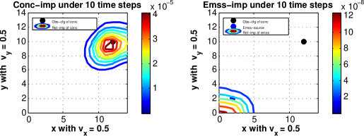
Figure 1: Advection test with data assimilation (DA) window $10\triangle t$ and southwest wind. Isopleths of ensemble relative improvements of the concentration and emission rate are shown in the leftside and rightside figures respectively.

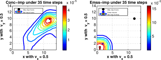
Figure 2: Advection test with DA window $35\triangle t$ and southwest wind. Plotting conventions are as in Fig. 1.

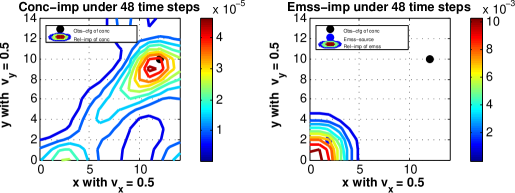
Figure 3: Advection test with DA window $48\triangle t$ and southwest wind. Plotting conventions are as in Fig. 1.

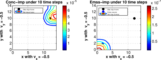
Figure 4: Advection test with DA window $10\triangle t$ and northeast wind. Plotting conventions are as in Fig. 1.

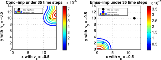
Figure 5: Advection test with DA window $35\triangle t$ and northeast wind. Plotting conventions are as in Fig. 1.

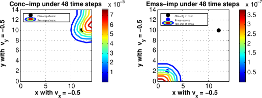
Figure 6: Advection test with DA window $48\triangle t$ and northeast wind. Plotting conventions are as in Fig. 1.

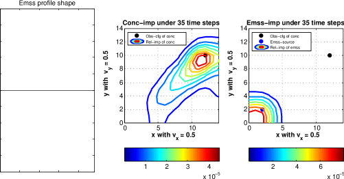
Figure 7: Emission signal test (weak) with DA window $35\triangle t$ and southwest wind. Plotting conventions are as in Fig. 1.

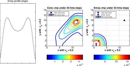
Figure 8: Emission signal test (strong) with DA window $35\triangle t$ and southwest wind. Plotting conventions are as in Fig. 1.

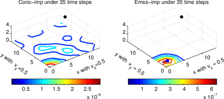
Figure 9: Diffusion test (weak) with DA window $35\triangle t$ and southwest wind. Plotting conventions are as in Fig. 1.

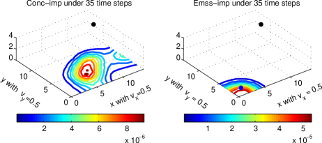
Figure 10: Diffusion test (strong) with DA window $35\triangle t$ and southwest wind. Plotting conventions are as in Fig. 1.

	$\tilde{p}^{c}$	$\tilde{p}^{e}$
Fig. 1	0.9979	0.0021
Fig. 2	0.5107	0.4893
Fig. 3	0.0345	0.9655

Table 1:

	$\tilde{p}^{c}$	$\tilde{p}^{e}$
Fig. 4	0.9977	0.0023
Fig. 5	0.9974	0.0026
Fig. 6	0.9974	0.0026

Table 2:

	$\tilde{p}^{c}$	$\tilde{p}^{e}$
Fig. 7	0.6811	0.3189
Fig. 8	0.5107	0.4893

Table 3:

	$\tilde{p}^{c}$	$\tilde{p}^{e}$
Fig. 9	0.9977	0.0023
Fig. 10	0.7755	0.2245

Table 4:

	$\tilde{P}_{low}^{c}$	$\tilde{P}_{low}^{e}$
Fig. 2	$2.8435\times 10^{-6}$	$2.3530\times 10^{-6}$
Fig. 9	$2.3850\times 10^{-7}$	$2.1627\times 10^{-8}$
Fig. 10	$7.8820\times 10^{-7}$	$1.5946\times 10^{-6}$

Table 5: $\tilde{P}_{low}^{c}$ and $\tilde{P}_{low}^{e}$ are respectively the total improvement values of the concentration and emission rates in the lowest layer

5 Sensitivity of observation networks to the initial state and emission rates

From the above discussion, we can determine the efficiency of the observation network by evaluating the improvement of estimation of initial state and emission rates separately, before we run the data assimilation by Kalman filer and smoother. However, it does not provide the information about the improved configurations of observations which can help improving the estimations. In this section, independent of any concrete data assimilation method, we will introduce the singular vector approach to identify the sensitive directions of observations to the initial state and emission rates.

Consider the generalized discrete-time linear system:

$$\delta x(t_{k+1})=M(t_{k+1},t_{k})\delta x(t_{k}),$$

where $\delta x(t_{0})=x(t_{0})-\hat{x}(t_{0})$, $\hat{x}(t_{0})$ is any estimate of $x(t_{0})$.

Assume the observation mapping is accurate, which implies the data is the only source of observation errors, we have

$$\delta y(t_{k})=H(t_{k})\delta x(t_{k}).$$

Define the magnitude of the perturbation of the initial state by the norm in the state space with respect to a positive definite matrix $W_{0}$

$$\|\delta x(t_{0})\|_{W_{0}}^{2}=\langle\delta x(t_{0}),W_{0}\delta x(t_{0})\rangle.$$

Similarly, we define the magnitude of the related observations perturbation in the time interval $[t_{0},\cdots,t_{N}]$ by the norm with respect to a sequence of positive definite matrix $\{W(t_{k})\}_{k=1}^{N}$

$$\|\delta y\|_{\{W(t_{k})\}}^{2}=\sum_{k=0}^{N}\langle\delta y(t_{k}),W(t_{k})\delta y(t_{k})\rangle,$$

where $\delta y(t_{k})=H(t_{k})\delta x(t_{k})$.

In order to find the direction of observation configuration which can minimize the perturbation of the initial states, the ratio

$$\dfrac{{\|\delta x(t_{0})\|_{W_{0}}^{2}}}{\|\delta y\|_{\{W(t_{k})\}}^{2}},\quad\delta y\neq 0$$

should be minimized. It is equivalent to maximize the ratio of the magnitude of observation perturbation and the initial perturbation

$$\dfrac{\|\delta y\|_{\{W(t_{k})\}}^{2}}{\|\delta x(t_{0})\|_{W_{0}}^{2}},\quad\delta x(t_{0})\neq 0.$$

Thus, we define the measure the perturbation growth as

$$g^{2}=\dfrac{\|\delta y\|_{\{W(t_{k})\}}^{2}}{\|\delta x(t_{0})\|_{W_{0}}^{2}}$$

$$= \sum_{k=0}^{N}\dfrac{\langle\delta y(t_{k}),W(t_{k})\delta y(t_{k})\rangle}{\langle\delta x(t_{0}),W_{0}\delta x(t_{0})\rangle}$$

$$= \sum_{k=0}^{N}\dfrac{\langle H(t_{k})\delta x(t_{k}),W(t_{k})H(t_{k})\delta x(t_{k})\rangle}{\langle\delta x(t_{0}),W_{0}\delta x(t_{0})\rangle}$$

$$= \sum_{k=0}^{N}\dfrac{\langle\delta x(t_{k}),H(t_{k})^{T}W(t_{k})H(t_{k})\delta x(t_{k})\rangle}{\langle\delta x(t_{0}),W_{0}\delta x(t_{0})\rangle}$$

$$= \sum_{k=0}^{N}\dfrac{\langle\delta x(t_{0}),M(t_{k},t_{0})^{T}H(t_{k})W(t_{k})H(t_{k})M(t_{k},t_{0})\delta x(t_{0})\rangle}{\langle\delta x(t_{0}),W_{0}\delta x(t_{0})\rangle}$$

$$= \dfrac{\langle\delta x(t_{0}),\sum_{k=0}^{N}M(t_{k},t_{0})^{T}H(t_{k})^{T}W(t_{k})H(t_{k})M(t_{k},t_{0})\delta x(t_{0})\rangle}{\langle\delta x(t_{0}),W_{0}\delta x(t_{0})\rangle}.$$

According to Liao and Sandu ([18]), singular vectors refer to the directions of the error growth in a descend sequence with respect to the descent singular values. Hence, in order to search the maximal directions of

$$g^{2}=\dfrac{\langle\delta x(t_{0}),\mathcal{G}^{T}\mathcal{W}\mathcal{G}\delta x(t_{0})\rangle}{\langle\delta x(t_{0}),W_{0}\delta x(t_{0})\rangle},\ \ \delta x(t_{0})\neq 0,$$

where $\mathcal{W}=\text{diag}(W(t_{0}),\cdots,W(t_{N}))$, $\mathcal{G}$ and $\mathcal{R}^{-1}$ have the same definitions with those in Section 3, we need to find out the solutions of the singular value problem:

$$W_{0}^{-\frac{1}{2}}\mathcal{G}^{T}\mathcal{W}\mathcal{G}W_{0}^{-\frac{1}{2}}v_{k}=s_{k}^{2}v_{k},\quad\mathcal{G}W_{0}\mathcal{G}^{T}u_{k}=s_{k}^{2}u_{k},$$

where $s_{1}\geqslant s_{2}\geqslant\cdots\geqslant s_{n}\geqslant 0$, $\{v_{k}\}_{i=1}^{n}$ and $\{u_{k}\}_{i=1}^{n}$ are the corresponding orthogonal singular vectors. Then, $\max_{\delta x(t_{0})\neq 0}g^{2}=s_{1}^{2}.$

Especially, if the perturbation norms are provided by the choice $W_{0}=P^{-1}(t_{0}|t_{-1})$ and $\mathcal{W}=\mathcal{R}^{-1}$ defined in Section 3,

$$g^{2}=\dfrac{\langle\delta x(t_{0}),\mathcal{G}^{T}\mathcal{R}^{-1}\mathcal{G}\delta x(t_{0})\rangle}{\langle\delta x(t_{0}),P^{-1}(t_{0}|t_{-1})\delta x(t_{0})\rangle},\ \ \delta x(t_{0})\neq 0.$$

We need to search the directions of

$$P^{\frac{1}{2}}(t_{0}|t_{-1})\mathcal{G}^{T}\mathcal{R}^{-1}\mathcal{G}P^{\frac{1}{2}}(t_{0}|t_{-1})v_{k}=s_{k}^{2}v_{k};$$ (30)

$$\mathcal{G}P^{-1}(t_{0}|t_{-1})\mathcal{G}^{T}u_{k}=s_{k}^{2}u_{k},\ \ k=1,\cdots,n.$$

Associated with (16), it is easy to find that the singular vector $v_{k}$ in (30), which is the direction of $\text{k}^{\text{th}}$-fast growth of the perturbation of observations evolved from the initial perturbation, is also the $\text{k}^{\text{th}}$ direction which maximize the improvement of estimation by Kalman filter and smoother (16), though the exact value of the eigenvalue of (16) related to $v_{k}$ is $\frac{s_{k}^{2}}{1+s_{k}^{2}}$ rather than the eigenvalue $s_{k}^{2}$ of (30). Meanwhile, we can find that the leading singular value $s_{1}$ is related to the operator norm of $\tilde{P}$ as

$$\|\tilde{P}\|=\max_{\|x\|=1}\|\tilde{P}x\|=\frac{s_{1}^{2}}{1+s_{1}^{2}}.$$

In addition, the similar analysis for the continuous-time system is presented in the appendix B.

6 Discussion

In the present work, approaches for determining the efficiency and sensitivity of observation configurations for the initial state and emission rates are established. Actually, to deal with the specific questions in atmospheric chemistry, some special operators are usually applied. For example, in order to consider the efficiency and sensitivity of observations in some certain locations, the local projection operator introduced by Buizza et al. ([4]) can be applied into approaches in Section 4 and Section 5.

Let $L$ be the $0-1$ diagonal matrix defined as

$$L_{ii}=\{\begin{array}[]{cc}1,&\ l_{i}\in L_{a},\\ 0,&\text{otherwise.}\end{array}$$

where $L_{a}$ is a fixed area and $l_{i}$ is the coordinate of $i^{\text{th}}$ grid point.

To test the efficiency and sensitivity of observation configurations in a special area, by rearranging the observations $y$ according to the locations, $\mathcal{G}$ in (12) should be defined as

$$\mathcal{G}=\left(\begin{array}[]{cc}LH(t_{0})M(t_{0},t_{0})\\ LH(t_{1})M(t_{1},t_{0})\\ \vdots\\ LH(t_{N})M(t_{N},t_{0})\end{array}\right).$$ (31)

If $LH(\cdot)$ is considered as the observation mapping, approaches in Section 3 and 5 can be applied.

In addition, if there is a multiplication of emission rates in the following model

$$\frac{d\delta c}{dt}=\mathbf{A}\delta c+B(t)\delta e(t),$$

then all approaches can also be applied into the extended model

$$\left(\begin{array}[]{c}\delta c(t)\\ \delta e(t)\end{array}\right)=\left(\begin{array}[]{cc}M(t,t_{0})&\int_{t_{0}}^{t}M(t,s)B(s)M_{e}(s,t_{0})ds\\ 0&M_{e}(t,t_{0})\end{array}\right)\left(\begin{array}[]{c}\delta c(t_{0})\\ \delta e(t_{0})\end{array}\right).$$

Appendix A The efficiency of observation networks for continuous-time systems

Consider the abstract continuous-time system

$$x(t)=M(t,t_{0})x(t_{0})+\varepsilon(t),$$

$$y(t)=H(t)x(t)+\nu(t),$$

where $x\in\mathds{R}^{n}$ is the state variable, $y\in\mathds{R}^{m}$ is observation vector at time $t$, the model error $\varepsilon(t)$ and the observation error $\nu(t)$, $t\in[t_{0},t_{N}]$ follow Gaussian distribution with zero mean, while $Q(t)$ and $R(t)$ are their covariance matrices respectively.

As in Section 3, we ignore the model error. It is well known that for the continuous Kalman filter, the covariance $P(t)$ of the optimal estimation of the state at time $t$ satisfies the integral Riccati equation

$$P(t|t)=M_{K}(t,t_{0})P(t_{0}|t_{-1})M_{K}^{T}(t,t_{0})+\int_{t_{0}}^{t}M_{K}(t,s)K(s)R(s)K^{T}(s)M_{K}^{T}(t,s)ds,$$

where $K(t)=P(t|t)H(t)R^{-1}(t)$ and $M_{K}(t,t_{0})=M(t,t_{0})-\int_{t_{0}}^{t}M(t,s)K(s)H(s)M_{K}(s,t_{0})ds$.

On one hand,

$$M_{K}(t,t_{0})P(t_{0}|t_{-1})M_{K}^{T}(t,t_{0})$$

$$= M(t,t_{0})P(t_{0}|t_{-1})M_{K}^{T}(t,t_{0})-\int_{t_{0}}^{t}M(t,s)K(s)H(s)M_{K}(s,t_{0})P(t_{0}|t_{-1})M_{K}^{T}(t,t_{0})ds$$

$$= M(t,t_{0})P(t_{0}|t_{-1})M_{K}^{T}(t,t_{0})-\int_{t_{0}}^{t}M(t,s)K(s)H(s)P(s|s)M_{K}^{T}(t,s)ds$$

$$+\int_{t_{0}}^{t}\int_{t_{0}}^{s}M(t,s)K(s)H(s)M_{K}(s,\eta)K(\eta)R(\eta)K^{T}(\eta)M_{K}^{T}(t,\eta)d\eta ds.$$

On the other hand,

$$\int_{t_{0}}^{t}M_{K}(t,s)K(s)R(s)K^{T}(s)M_{K}^{T}(t,s)ds$$

$$= \int_{t_{0}}^{t}[M(t,s)-\int_{s}^{t}M(t,\eta)K(\eta)H(\eta)M_{K}(\eta,s)d\eta]K(s)R(s)K^{T}(s)M_{K}^{T}(t,s)ds$$

$$= \int_{t_{0}}^{t}M(t,s)K(s)R(s)K^{T}(s)M_{K}^{T}(t,s)ds$$

$$-\int_{t_{0}}^{t}\int_{0}^{\eta}M(t,\eta)K(\eta)H(\eta)M_{K}(\eta,s)K(s)R(s)K^{T}(s)M_{K}^{T}(t,s)dsd\eta$$

$$= \int_{t_{0}}^{t}M(t,s)K(s)R(s)K^{T}(s)M_{K}^{T}(t,s)ds$$

$$-\int_{t_{0}}^{t}\int_{0}^{s}M(t,s)K(s)H(s)M_{K}(s,\eta)K(\eta)R(\eta)K^{T}(\eta)M_{K}^{T}(t,\eta)d\eta ds.$$

Therefore, $P(t|t)=M(t,t_{0})P(t_{0}|t_{-1})M_{K}^{T}(t,t_{0})$.

Since

$$M^{-1}(t,t_{0})=M_{K}^{-1}(t,t_{0})M_{K}(t,t_{0})M^{-1}(t,t_{0})$$

$$= M_{K}^{-1}(t,t_{0})[M(t,t_{0})-\int_{t_{0}}^{t}M_{K}(t,s)K(s)H(s)M(s,t_{0})ds]M^{-1}(t,t_{0})$$

$$= M_{K}^{-1}(t,t_{0})-\int_{t_{0}}^{t}M_{K}^{-1}(s,t_{0})L(s)H(s)M(t,s)ds,$$

we obtain $M_{K}^{-1}(t,t_{0})=M^{-1}(t,t_{0})+\int_{t_{0}}^{t}M_{K}^{-1}(s,t_{0})K(s)H(s)M^{-1}(t,s)ds$.

Define $\hat{x}(t_{0}|t)=E[x(t_{0})|y(s),s\in[t_{0},t]]$ and denote its covariance matrix as

$$P(t_{0}|t)=E[(x(t_{0})-\hat{x}(t_{0}|t))(x(t_{0})-\hat{x}(t_{0}|t))^{T}],$$

Hence,

$$P^{-1}(t_{0}|t)$$

$$= [M^{-1}(t,t_{0})P(t|t)M^{-T}(t,t_{0})]^{-1}$$

$$= [P(t_{0}|t_{-1})M_{K}^{T}(t,t_{0})M^{-T}(t,t_{0})]^{-1}$$

$$= M^{T}(t,t_{0})[M^{-T}(t,t_{0})+\int_{t_{0}}^{t}M^{-T}(t,s)H^{T}(s)K^{T}(s)M_{K}^{-T}(s,t_{0})ds]P(t_{0}|t_{-1})^{-1}$$

$$= P^{-1}(t_{0}|t_{-1})+\int_{t_{0}}^{t}M^{T}(s,t_{0})H^{T}(s)R^{-1}(s)H(s)M(s,t_{0})ds.$$

Let $t=t_{N}$ and define the observability mapping $\mathcal{G}:\mathds{R}^{n}\rightarrow\mathcal{L}^{2}([t_{0},t_{N}];\mathds{R}^{m})$ as

$$\mathcal{G}f:=H(\cdot)M(\cdot,t_{0})f,\quad f\in\mathds{R}^{n},$$

its adjoint operator $\mathcal{G}^{*}$ is

$$\mathcal{G}^{*}f=-\int_{t_{N}}^{t_{0}}M^{T}(s,t_{0})H^{T}(s)f(s)ds,\quad f\in L^{2}([t_{0},t_{N}];\mathds{R}^{m}).$$

Further, we define $\mathcal{R}^{-1}:\mathcal{L}^{2}([t_{0},t_{N}];\mathds{R}^{m})\rightarrow\mathcal{L}^{2}([t_{0},t_{N}];\mathds{R}^{m})$,

$$\mathcal{R}^{-1}f:=R^{-1}(\cdot)f(\cdot),\quad f\in\mathcal{L}^{2}([t_{0},t_{N}];\mathds{R}^{m}).$$

Thus,

$$P^{-1}(t_{0}|t_{N})=P^{-1}(t_{0}|t_{-1})+\mathcal{G}^{*}\mathcal{R}^{-1}\mathcal{G},$$ (32)

where $\mathcal{G}^{*}\mathcal{R}^{-1}\mathcal{G}$ is the observability Gramian of continuous-time systems.

Obviously, (32) has the same pattern as (11), so

$$P^{-\frac{1}{2}}(t_{0}|t_{-1})(P(t_{0}|t_{-1})-P(t_{0}|t_{N}))P^{-\frac{1}{2}}(t_{0}|t_{-1})$$ (33)

$$= I-(I+P^{\frac{1}{2}}(t_{0}|t_{-1})\mathcal{G}^{T}\mathcal{R}^{-1}\mathcal{G}P^{\frac{1}{2}}(t_{0}|t_{-1}))^{-1}$$

$$= V(I-(I+S^{2})^{-1})V^{T},$$

where $VS^{2}V^{T}$ is the singular value decomposition of $P(t_{0}|t_{-1})^{\frac{1}{2}}\mathcal{G}^{T}\mathcal{R}^{-1}\mathcal{G}P(t_{0}|t_{-1})^{\frac{1}{2}}$.

Then, following the same steps as in Section 3, we can obtain the efficiency of observation configurations for continuous-time systems.

Appendix B The sensitivity of observation networks for continuous-time systems

Consider the generalized continuous-time linear system:

$$\delta x(t)=M(t,t_{0})\delta x(t_{0}),$$

with the corresponding forecast perturbation of observations evolving from $\delta x(t_{0})$

$$\delta y(t)=H(t)\delta x(t).$$

To be brief, let $W_{0}=P^{-1}(t_{0}|t_{-1})$ and $\mathcal{W}(t)=R^{-1}(t)$ (see Appendix A), and define the magnitude of the perturbation of the initial state and observations respectively by

$$\|\delta x(t_{0})\|_{P^{-1}(t_{0}|t_{-1})}^{2}=\langle\delta x(t_{0}),P^{-1}(t_{0}|t_{-1})\delta x(t_{0})\rangle,$$

$$\|\delta y\|_{\{R^{-1}(t)\}}^{2}=\int_{t_{0}}^{t_{N}}\langle\delta y(t),R^{-1}(t)\delta y(t)\rangle dt.$$

Thus, the perturbation growth for continuous-time system can be measured by

$$g^{2}=\dfrac{\|\delta y\|_{\{R^{-1}(t))\}}^{2}}{\|\delta x(t_{0})\|_{P^{-1}(t_{0}|t_{-1})}^{2}}$$

$$= \dfrac{\int_{t_{0}}^{t_{N}}\langle H(t)\delta x(t),R^{-1}(t)H(t)\delta x(t)\rangle dt}{\langle\delta x(t_{0}),P^{-1}(t_{0}|t_{-1})\delta x(t_{0})\rangle}$$

$$= \dfrac{\langle\delta x(t_{0}),\int_{t_{0}}^{t_{N}}M(t,t_{0})^{T}H(t)^{T}R^{-1}(t)H(t)M(t,t_{0})\delta x(t_{0})dt\rangle}{\langle\delta x(t_{0}),P^{-1}(t_{0}|t_{-1})\delta x(t_{0})\rangle}$$

$$= \dfrac{\langle\delta x(t_{0}),\mathcal{G}^{*}\mathcal{R}^{-1}\mathcal{G}\delta x(t_{0})\rangle}{\langle\delta x(t_{0}),P^{-1}(t_{0}|t_{-1})\delta x(t_{0})\rangle},\ \ \ \delta x(t_{0})\neq 0,$$

where $\mathcal{G}$ and $\mathcal{R}^{-1}$ are defined in Appendix A.

To find the directions maximizing the ratio, we need to find the solutions of the singular value problem:

$$P^{\frac{1}{2}}(t_{0}|t_{-1})\mathcal{G}^{T}\mathcal{R}^{-1}\mathcal{G}P^{\frac{1}{2}}(t_{0}|t_{-1})v_{k}=s_{k}^{2}v_{k},$$ (34)

$$\mathcal{G}P^{-1}(t_{0}|t_{-1})\mathcal{G}^{T}u_{k}=s_{k}^{2}u_{k}.$$ (35)

where $s_{1}\geqslant s_{2}\geqslant\cdots\geqslant s_{n}\geqslant 0$, $\{v_{k}\}_{i=1}^{n}$ and $\{u_{k}\}_{i=1}^{n}$ are orthogonal singular vectors.

Compared (34) with (33) in Appendix A, similar analysis and conclusions as Section 5 can be extended to continuous-time systems.

References

• [1] J. Barkmeijer, M. V. Gijzen and F. Bouttier, Singular vectors and estimates of the analysis-error covariance metric, Q. J. Roy. Meteorol. Soc., 124, pp. 1695–1713, 1998.
• [2] M. Bocquet and P. Sakov, Joint state and parameter estimation with an iterative ensemble Kalman smoother, Nonlinear proc geoph., vol. 20, pp. 803–818, 2013.
• [3] R. Buizza, Localization of optimal perturbations using a projection operator, Quart. J. Roy. Meteor. Soc., 120, pp. 1647–1681, 1994.
• [4] R. Buizza and A. Montani, Targeting observations using singular vectors, J. Atmos. Sci, vol 56, pp. 2965–2985, 1999.
• [5] R. Buizza, J. Barkmeijer, T. N. Palmer and D. S. Richardson, Current status and future developments of the ECMWF Ensemble Prediction System, Meteorol. Appl. 7, pp. 163–175, 2000.
• [6] R. Buizza, T. N. Palmer, The singular-vector structure of the atmospheric global circulation, J. Atom. Sci., vol. 52, No. 9, pp. 1434–1456, 1995.
• [7] D. E. Catlin, Estimation, control, and the discrete Kalman filter, Springer-Verlag, 1989.
• [8] R. Daley, Atmospheric data analysis, Cambridge University Press, 1991.
• [9] H. Elbern and H. Schmidt, A four–dimensional variational chemistry data assimilation scheme for Eulerian chemistry transport modeling, J. Geophys. Res., 104, 18 583–598, 1999.
• [10] H. Elbern and H. Schmidt and O. Talagrand and A. Ebel, 4D-variational data assimilation with an adjoint air quality model for emission analysis, Environ modell softw, vol. 15, pp. 539–548, 2000.
• [11] H. Elbern, A. Strunk, H. Schmidt and O. Talagrand, Emission rate and chemical state estimation by 4-dimension variational inversion, Atmos. Chem. Phys., vol. 7, pp. 3749–3769, 2007.
• [12] G. Evensen, Data assimilation: The ensemble Kalman filter, 2th Edition, Springer, 2009.
• [13] A. Gelb (ed.), Applied Optimal Estimation, Cambridge, Mass.: M.I.T. Press, 1974.
• [14] N. Goris, H. Elbern, Singular vector decomposition for sensitivity analyses of tropospheric chemical scenarios, Atmos. Chem. Phys., vol. 13, pp. 5063–5087, 2013.
• [15] F. M. Ham and R. G. Brown, Observability, eigenvalues and Kalman filtering, IEEE Tran. Aero. and Electronic sys. VOL. AES-19, NO. 2, 1983.
• [16] C. D. Johnson, Optimization of a certain quality of complete controllability and observability for linear dynamic systems, Trans. ASME, vol. 91, series D, pp. 228–238,1969.
• [17] B. B. Khattatov, J. Gille, L. Lyjak, G. Brasseur, V. Dvortsov, A. Roche and J. Waters, Assimilation of photochemically active species and a case analysis of UARS data, J. Geophys. Res., vol. 22, pp. 18715–18738, 1999.
• [18] W. Liao, A. Sandu, G. R. Carmichael and T. Chai, Singular vector analysis for atmospheric chemical transport models, Month. Weather Rev., vol. 134, pp. 2443–2465, 2006.
• [19] R. E. Kalman, A new approach to linear filtering and prediction problems, J. Basic Engineering, pp. 35–45, Mar. 1960.
• [20] R. E .Kalman, R. S. Bucy, New results in linear filtering and prediction theory, J. Basic Engineering, pp. 95–108, Mar. 1961.
• [21] E. N. Lorenz, A study of the predictability of a 28 variable atmospheric model, Tellus, vol. 17, pp. 321–333, 1965.
• [22] D. F. Morrison, Multivariate Statistical Methods, New York: McGraw-Hill, 1967.
• [23] X. Tang, J. Zhu, Z. F. Wangand and A. Gbaguidi, Improvement of ozone forecast over Beijing based on ensemble Kalman filter with simultaneous adjustment of initial conditions and emissions, Atmos. Chem. Phys., vol. 11, pp. 12901–12916, 2011.
• [24] M. A. Woodbury, Inverting modified matrices, Memorandum Rept. 42, Statistical Research Group, Princeton University, Princeton, NJ, 1950.
• [25] N. N. Yanenko, The method of fractional steps: solution of problems of mathematical physics in several variables, Springer, 1971.