Random matrix approach to multivariate categorical data analysis

Abstract

Correlation and similarity measures are widely used in all the areas of sciences and social sciences. Often the variables are not numbers but are instead qualitative descriptors called categorical data. We define and study similarity matrix, as a measure of similarity, for the case of categorical data. This is of interest due to a deluge of categorical data, such as movie ratings, top-10 rankings and data from social media, in the public domain that require analysis. We show that the statistical properties of the spectra of similarity matrices, constructed from categorical data, follow those from random matrix theory. We demonstrate this approach by applying it to the data of Indian general elections and sea level pressures in North Atlantic ocean.

1 Introduction

Study of correlations is an integral part of almost every branch of science and social science. Correlated systems and phenomena, such as in non-equilibrium systems, present a rich variety of behaviour not normally seen in uncorrelated systems. Global climate patterns depend on the spatial and temporal correlations among atmospheric variables [1], correlations in the stock market records indicate clustering of stocks and indices [2, 3, 4, 5], correlations among EEG channels might indicate health of the subject [6, 7]. In computer science, correlations are an integral part of most clustering algorithms [8]. In these examples, the object of central interest is the same-time correlation function $\langle x(t)y(t)\rangle$ for two stationary stochastic processes $x(t)$ and $y(t)$ with zero mean. The processes $x_{t}$ and $y_{t}$ could be measured data or generated through simulations. When $N$ variables $x_{i}(t),i=1,2,...N$ are present, the correlation matrix $C$ is the appropriate generalisation in which any matrix element $c_{ij}$ represents the correlation between the variables $x_{i}(t)$ and $x_{j}(t)$ [9]. It must be noted that singular value decomposition, empirical orthogonal functions, Karhunen-Loeve decomposition are all variants of this correlation matrix approach.

Random matrix theory (RMT) [10] has emerged as an important tool to understand the spectra of correlation matrices [7]. It is by now well established that the spectra of empirical correlation matrix, for most part, is well described by random matrix results [2, 3, 4, 5, 6, 7, 11, 12, 13]. Deviations from random matrix behaviour indicate the presence of significant information [4] that cannot be explained purely by assumptions of randomness in matrix elements. All these methods and analysis, based on correlations and RMT, depend on the variables $x_{i}(t)$ being a series of numbers, representing some possibly stochastic phenomena.

The main objective of this paper is to analyse a measure of association or similarity for multivariate data sets that are not numbers but discrete qualitative indicators. Movie ratings and top-ten rankings are some examples of qualitative indicators. Even more challenging cases arise when discrete indicators cannot be ranked in any numerical order. For instance, the responses in an opinion poll cannot be assigned any meaningful ranking order. All such data sets are called categorical data [14]. In the context of deluge of data of various kinds available in the public domain over the internet, it is imperative to look for methods to effectively analyse categorical data. One important application is in the analysis of data from social media such as facebook posts, twitter updates, blogs etc., which are mostly not in numerical form. Social media analysis is now widely used by corporates and even governments to understand the public perception of their brand value, products and services. Hence, computing measures of association with such non-numerical data is often necessary. Recently, random walks and network theory have been used for computing such measures [15]. In contrast, here we develop a statistical technique that is analogous to correlation matrix formalism and apply RMT tools.

Generally, multivariate empirical data is highly noisy and redundant. Thus, it is important to separate the information content from noise components. To do this, we obtain similarity matrix $\mathbf{S}$ as a multivariate generalisation of similarity measure. We note that similarity matrix $\mathbf{S}$ is widely applied in clustering algorithms in computer sciences [8] and for classifying genetic data [16]. By comparing the statistical properties of spectra of $\mathbf{S}$ with that from an appropriate ensemble of RMT we can identify the eigenvalues and the eigenmodes that are random. The spectral components that deviate from RMT results are not random and generally contain system-specific information yielding valuable information about the system. We apply the formalism to two real-world systems, (i) analysis of Indian general elections results, (ii) mean sea level pressure over North Atlantic region.

2 Formalism

In this section, we introduce the formalism for a similarity measure and its multivariate generalisation. We consider time series $x_{t}$ of categorical data. The elements of the time series are chosen from $p$ possible objects denoted by numbers $1-p$. Note that the labels $1-p$ do not affect the value of the measure. For example, $x_{t}$ could be the time series of parties winning elections in a city. If there were only two parties (objects) denoted by 1 and 2 that have won election in that city, then the time series could take the form, $x_{t}=1,2,1,1,2,1,2,2,1...$. For the case of two time series $x_{t}$ and $y_{t}$ of length $T$, we define the similarity measure as

$$c_{\textnormal{xy}}=\mathcal{N}\displaystyle\sum_{t=1}^{T}w_{t}~{}\delta_{x_{t},y_{t}}$$ (1)

where normalisation constant is $\mathcal{N}=\sum_{t=1}^{T}w_{t}$ and $\delta_{x_{t},y_{t}}$ is the Kronecker delta ($\delta_{a,b}=1$ if $a=b$, $0$ if $a\neq b$). In this, $w_{i}$ are the weights assigned to each data point. In most applications, every data point is given equal weightage and hence $w_{t}=1$, for all $t=1,2,3...T$. Clearly, $c_{\textnormal{xy}}=1$ only if $x_{t}=y_{t},\forall~{}t$. If $c_{\textnormal{xy}}=0$, this implies $x_{t}\neq y_{t},\forall~{}t$. If $0<c_{\textnormal{xy}}<1$, it indicates that $x_{t}$ and $y_{t}$ are dissimilar to varying extents. Note that $c_{\textnormal{xy}}$ is similar to Jaccard index [17, 18] used to measure similarity of finite sample sets.

Next, we consider a multivariate scenario with $N$ variables $x_{i},i=1,2,....N$, each being a time series of length $T$. This can be elegantly handled in matrix notation. Let $\mathbf{D}$ represent a data matrix with of $T$ rows and $N$ columns. Each column is a time series. We define a new operator ”$\ast$”, through its action on two vectors $\mathbf{a}=(a_{1}~{}a_{2}\ldots a_{T})$ and $\mathbf{b}=(b_{1}~{}b_{2}\ldots b_{T})$, defined as

$$\mathbf{a}^{T}\ast\mathbf{b}=\delta_{a_{1},b_{1}}+\delta_{a_{2},b_{2}}+\ldots\delta_{a_{T},b_{T}}.$$ (2)

This is similar to applying element-wise AND logical operation between the two vectors. Using this operator, the multivariate generalisation of similarity measure is

$$\mathbf{S}=\mathbf{D}^{T}\ast\mathbf{D}$$ (3)

In this form, $\mathbf{S}$ has a structure similar to that of Wishart matrix $C=D^{T}D$ in multivariate statistics [19]. In particular, $\mathbf{S}$ is also a positive definite matrix with eigenvalues $\lambda\geq 0$. To study the spectra of $\mathbf{S}$, we numerically solve the eigenvalue equation $\mathbf{Sx}_{i}=\lambda_{i}\mathbf{x}_{i}$ and obtain its eigenvalues $\lambda_{i}$ and the eigenvectors $\mathbf{x}_{i}$.

3 Similarity matrix

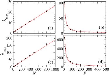
Figure 1: (Colour online) Numerically computed $\lambda_{\textnormal{max}}$ (circles) as a function of number of variables $N$ (left) and number of objects $p$ (right). (a,b) are for uniform distribution and (c,d) are for geometric distribution of random numbers. The solid lines are the analytical results in Eqs. 9 and 11.

This formalism can be illustrated with a simple solvable model. Consider $p$ discrete objects, labelled 1 to $p$, and $N$ random variables. Each variable $x_{i}(t),i=1,2,...N$ is a time series with elements drawn from a discrete probability distribution $P(\phi)$ for $\phi=1,2,3\dots p$ and $P(\phi)=0$ otherwise. Then, the elements of $\mathbf{S}$ will be

$$s_{ij}=\frac{1}{T}~{}\sum_{t=1}^{T}\sum_{\phi^{\prime}=1}^{p}\sum_{\phi=1}^{p}P_{i}(\phi)~{}P_{j}(\phi^{\prime})~{}\delta_{\phi,\phi^{\prime}}$$ (4)

Note that $s_{ij}$ turns out to be some function of $p$. Clearly, by construction, the diagonal elements are $s_{ii}=(1/T)\sum_{t}\sum_{\phi}P_{i}(\phi)=1$. In the limit $T\to\infty$, $s_{ij}$ would have converged and we get $\mathbf{S}$ to be a matrix of order $N$ and of the form

$$\mathbf{S}=\begin{pmatrix}1&a&a&...\\ a&1&a&...\\ a&a&1&...\\ :&:&:&1\\ \end{pmatrix}.$$ (5)

The off-diagonal elements are $s_{ij}=a=a(p)$. The eigenvalues of $\mathbf{S}$ can be analytically obtained. There are only two distinct eigenvalues

$$\lambda_{max}=1+(N-1)a,\;\;\;\mbox{and}\;\;\;\lambda_{1}=1-a.$$ (6)

This simple estimate shows that $\lambda_{max}$ is the dominant eigenvalue and the other eigenvalue is $N-1$ fold degenerate. We also note that the normalised eigenvector corresponding to $\lambda_{max}$ is

$$(1/\sqrt{N})(1~{}1~{}1.....1~{}1).$$ (7)

Now, we can apply this formalism to the case in which the time series $x_{i}(t)$ are drawn from a discrete uniform distribution of the form

$$P(\phi)=\frac{1}{p},\;\;\;\;\;\;\phi=1,2\ldots p.$$ (8)

Then, using Eq. 4, the elements of similarity matrix is $s_{ij}=a=1/p$ for all $i\neq j$. Then, the eigenvalues are

$$\lambda_{max}=1+(N-1)/p~{}~{}~{}~{}\mbox{and}~{}~{}~{}~{}\lambda_{1}=1-1/p.$$ (9)

Next, we consider geometric distribution given by,

$$P(\phi)=(1-q)^{\phi}q,\;\;\;\;\;\;\phi=1,2,3\ldots,$$ (10)

where $0<q\leq 1$. Note that unlike the uniform distribution (Eq. 8), the geometric distribution has infinite support. Hence we choose $q$ such that $\phi=1,2,3\dots p$ such that $1-\sum_{\phi=1}^{p}P(\phi)<10^{-4}$. Then, $a\approx q/(2-q)$. Using an empirical relation we obtained $q\approx 6/p^{0.8}$, we get $s_{ij}=a\approx 3/(p^{0.8}-3)$. Then, the eigenvalues are

$$\lambda_{max}\approx 1+\frac{3(N-1)}{p^{0.8}-3}~{}~{}~{}~{}\mbox{and}~{}~{}~{}~{}\lambda_{1}\approx 1-\frac{3}{p^{0.8}-3}.$$ (11)

We will use these results as benchmarks to compare with the spectra computed from random similarity matrix.

4 Random similarity matrix

In this section, we will study the spectra of random similarity matrix $\mathbf{S_{R}}$ in detail. In particular, we compare the statistical properties of $\mathbf{S}$ with those obtained from the random similarity matrix. We define random similarity matrix $\mathbf{S_{R}}$ for the case of $p$ objects (labelled by integers 1 to $p$) and $N$ variables as follows. Let $\mathbf{D_{R}}$ be a matrix whose elements are independent and identically distributed integers in the range $[1-p]$ drawn from a discrete probability distribution function. Then, $\mathbf{S_{R}}=\mathbf{D_{R}}^{T}\ast\mathbf{D_{R}}$ is the random similarity matrix of order $N$.

First, we look at how the number of objects $p$ and number of variables $N$ affect the spectrum of $\mathbf{S_{R}}$. We consider $p=40$ and $p=400$ objects with $N=1000$ variables and length of time series being $T=2000$. All the simulation results (solid circles in Fig 1(a-d)) have been averaged over 100 realisations of appropriate similarity matrix. Fig. 1(a,b) shows the variation of $\lambda_{max}$ as a function of number of variables $N$ and number of objects $p$ for the case of uniform distribution. Surprisingly, the value of $\lambda_{max}$ predicted by Eq. 9, shown as solid line in this figure, holds good even when the elements of $\mathbf{S_{R}}$ are noisy due to finite length of time series. In Fig 1(c,d) shows $\lambda_{max}$ for the case of geometric distribution. In this case, the number of objects $p$ is approximate and yet the semi-analytical estimate for the dominant eigenvalue (Eq. 11) is in good agreement with the simulated results. In general, $\lambda_{max}$ decreases with $p$ because as the number of objects increases, the probability that two time series will have some common objects decays. For finite number of objects, this decay can be approximated as $p^{-1}$ for uniform and $p^{-0.8}$ for geometric distribution of random numbers. In the limit $p\to\infty$, there is only one distinct eigenvalue $\lambda=1$ and it is $N$-fold degenerate.

4.1 Eigenvalue Density

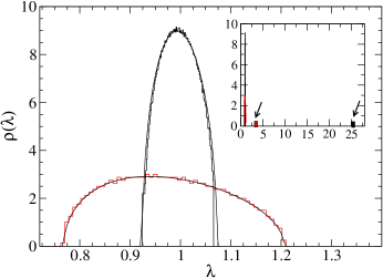
Figure 2: (Colour online) Eigenvalue density for $p=40$ and $p=400$. The histograms are from simulations and the solid curves represent Eq. 13. The inset shows part of the main graph to focus on the dominant eigenvalues (indicated by arrows) which are far from the bulk of eigenvalues.

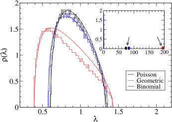
Figure 3: (Colour online) Eigenvalue density for $\mathbf{S_{R}}$ with random variables from discrete distributions, Poisson, Binomial and Geometric. Histograms are from simulations and solid lines are fitted using Eq. 13. Inset shows $\rho(\lambda)$ focussing on the dominant eigenvalues (highlighted by arrows).

We study two quantities that characterise the eigenvalues of $\mathbf{S_{R}}$, namely, eigenvalue density and spacing distribution. The mean density of eigenvalues is defined by

$$\rho(\lambda)=\sum_{i}\delta(\lambda-\lambda_{i}),$$ (12)

where $\delta(.)$ is the Dirac-delta function. Given that Eq. 3 has a structure similar to that of Wishart matrix, it is reasonable to expect the density of eigenvalues for random Wishart matrix $\mathbf{C}=\mathbf{D}^{\textnormal{T}}\mathbf{D}$ to hold good for random similarity matrix as well. In Wishart case, if $\mathbf{D_{R}}$ is a $T\times N$ random matrix with uncorrelated column vectors drawn from a Gaussian distribution with mean $\mu$ and variance $\sigma^{2}$, then $\rho(\lambda)$, in the limit $N\to\infty$ and $T\to\infty$ and $Q=\frac{T}{N}\geq 1$ is the Marchenko-Pastur law [19]

$$\rho(\lambda)=\frac{Q}{2\pi\sigma^{2}}\frac{\sqrt{(\lambda_{\textnormal{max}}-\lambda)(\lambda-\lambda_{\textnormal{min}})}}{\lambda},$$ (13)

for $\lambda\in[\lambda_{\textnormal{min}},\lambda_{\textnormal{max}}]$ and $\rho(\lambda)=0$ otherwise. In this, the largest and smallest eigenvalues are

$$\lambda_{\textnormal{max}/\textnormal{min}}=\lambda_{+/-}=\sigma^{2}(1+1/Q\pm 2\sqrt{1/Q}).$$ (14)

In the limit $Q=1$, the eigenvalue density leads to the well-known Wigner semi-circle law [20]. We compare Eq. 13 with eigenvalue density computed for random similarity matrix.

The eigenvalue density, for the bulk of eigenvalues, of random similarity matrix $\mathbf{S_{R}}$ is shown in Fig. 2 and it is well described by Eq. 13. On the other hand, the largest eigenvalue $\lambda_{max}$, highlighted in the inset of Fig. 2, is an order of magnitude larger than all the other eigenvalues. It stands out from the bulk. This is a unique spectral signature of random similarity matrix $\mathbf{S_{R}}$. A matrix such as $\mathbf{S_{R}}$ that encodes random correlations, in the spirit of random matrix theory, is not expected to accord special treatment for any part of the spectrum. Yet, the dominant eigenvalue $\lambda_{max}$ has a special place in the spectrum. The $\rho(\lambda)$ for Poisson, Binomial and Geometric distribution of random numbers shown in Fig. 3 also display a similar feature for $\lambda_{max}$. In this case too (Fig. 3) the bulk of eigenvalues are reasonably consistent with Eq. 13. The mild deviation for geometric distribution case in this figure can be attributed to the approximate nature of the calculation due to its infinite support.

4.2 Spacing distribution

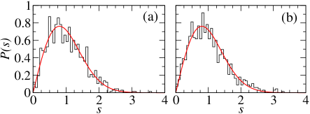
Figure 4: (Colour online) Empirical spacing distribution for the eigenvalues obtained from $\mathbf{S}$ with elements of $\mathbf{D}$ drawn from (a) uniform distribution and (b) geometric distribution. In both cases, $p=40,N=1000$ and $T=2000$. The solid curve is Wigner distribution (Eq. 15).

In this section, we present results for the spacing distribution of the eigenvalues. We remove the dominant eigenvalue $\lambda_{max}$ and compute spacing distribution using all the other eigenvalues in the bulk (see Figs. 2-3). If the eigenvalues of $\mathbf{S_{R}}$ are represented by $\lambda_{i},i=1,2,\dots N$, we transform the eigenvalues to obtain ’unfolded’ eigenvalues $\epsilon_{i},i=1,2,\dots N$, The nearest neighbour spacings are defined as $s_{i}=\epsilon_{i+1}-\epsilon_{i}$ such that $\langle s\rangle=1$. Given that $\mathbf{S_{R}}$ is real symmetric matrix with random entries, we expect the empirical spacing distribution obtained from the spectra of $\mathbf{S_{R}}$ to be best described by Gaussian Orthogonal Ensemble (GOE) result, the Wigner distribution, of random matrix theory [10]. Hence, the appropriate result is,

$$P_{W}(s)=\frac{\pi}{2}s~{}e^{-\frac{\pi}{4}s^{2}}.$$ (15)

In Fig. 4 we show the computed spacing distribution for the eigenvalues of $\mathbf{S_{R}}$ with the matrix elements of $\mathbf{D_{R}}$ drawn from discrete uniform and geometric distributions. For both these cases, the spacing distributions follow the random matrix theory results in Eq. 15. It must be recalled that similar results hold good for the spacing distribution of empirical correlation matrices [4, 21]. We further note that as $T\to\infty$, the matrix elements of $\mathbf{S_{R}}$ converge to their true values and the spacing distribution deviates strongly from Eq. 15.

4.3 Eigenvector statistics and Information Entropy

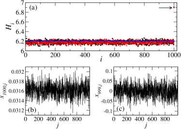
Figure 5: (Colour online) (a) Information entropy for the eigenvectors of $\mathbf{S_{R}}$ for the case of uniform distribution (black circle) and geometric distribution (red square). $H_{i}$ for the dominant eigenvector stands out from the bulk and is highlighted by an arrow. For the case of $\mathbf{S_{R}}$ obtained for the uniform distribution case (b) shows eigenvector of the dominant eigenvalue and (c) shows eigenvector for an eigenvalue in the bulk.

In this section, we study the properties of eigenvectors $\mathbf{x}_{i},i=1,2,...N$ of $\mathbf{S_{R}}$. The eigenvectors corresponding to the eigenvalues in the bulk are Gaussian distributed (not shown here), in accordance with the random matrix results [10]. A comprehensive comparison with random matrix results can be done by computing the information entropy for the $i$-th eigenvector defined by [22]

$$H_{i}=-\sum_{j}|x_{ij}|^{2}\ln|x_{ij}|^{2}.$$ (16)

The corresponding random matrix average for the information entropy is given by $H^{RMT}\sim\ln(N/2)$ [22], where $N$ is the dimension of the random matrix. We show the information entropy $H_{i}$ as a function of eigenvalue index $i$ in Fig. 5. The information entropy $H_{i}$ for the bulk of eigenvectors follow random matrix result $H_{i}\approx\ln 500=6.214$, indicated as a blue line. As an instance of such an eigenvector in the bulk, we show in Fig 5(c) the 999th eigenvector components $x_{999,j}$. The random nature of this eigenvector is clearly visible in its oscillations about zero. This behaviour must be contrasted with the dominant eigenvector (corresponding to $\lambda_{max}$) $x_{1000,j}$ shown in Fig 5(b). In this case, though the oscillations exist, they are not about zero, i.e, all the components of this eigenvector have identical phase. This behaviour can be understood based on the fact that for the simple model in Eq. 5, obtained in the $T\to\infty$ limit, the dominant eigenvector has the form shown in Eq. 7. Note that phases of all the components are identical in Eq. 7 as well. For the dominant eigenvector of $\mathbf{S_{R}}$ the amplitudes become random but not the phases. This non-random phases leads to significant deviation from random matrix average $H^{RMT}$ for information entropy as indicated by the arrow in Fig. 5(a). Thus, deviations from random matrix results imply presence of correlations either in the amplitude or the phase of the eigenvectors. This, in turn, could be traced to the correlations in the similarity measure for many variables.

5 Application

We apply the formalism to two different data sets, (i) the data of Indian general elections and (ii) atmospheric pressure in the region of North Atlantic ocean. We describe the motivations for choice of these data sets and their details below.

5.1 Elections data

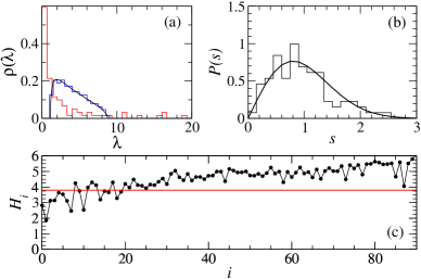
Figure 6: (Colour online) Results from the spectra of $\mathbf{S}$ obtained from data on Indian general elections. (a) Eigenvalue density for elections data compared against random similarity matrix, (b) spacing distribution obtained from elections data and (c) information entropy. See text for details.

The general elections held in India to elect the lower house of Indian parliament is the largest democratic exercise of its kind in the world with about 814.5 million people eligible to exercise their right to vote. These elections elect 543 representatives from as many constituencies to the lower house, Lok Sabha. For the purposes of our analysis, we identify 19 major political parties that have had significant representation in the elections held in India since 1984. These parties form our objects, i.e, $p=19$. For each constituency, the data we employ is a time series of winning party at seven general elections held during 1984-2004 and hence $T=7$. The number of variables is the number of constituencies, $N=543$. The general elections data, dating back to the first one in 1952, is provided by the Election Commission of India [23] and all the analysis reported here is based on this data. In this scenario, the similarity measure $s_{ij}$ is an index of how close are $i$-th and $j$-th constituencies in terms of the parties they have elected in the series of general elections. For instance, $s_{ij}=1$ implies that $i$-th and $j$-th constituencies have exactly chosen the same set of parties in all the general elections.

We note that the length of the time series is small and hence the computed matrix $\mathbf{S}$ is singular. This is also evident from the fact that out of 543 eigenvalues, only 91 of them are non-zero which form the basis for the results of eigenvalue statistics presented in Fig. 6(a,b). In Fig. 6(a), we show the computed eigenvalue density $\rho(\lambda)$. We note that unlike in the cases shown in Figs. 2 - 3, many eigenvalues, both at the lower and upper end, deviate from random matrix formula (Eq. 13). Even though the spacing distribution, shown in Fig. 6(b), largely follows Wigner distribution there are visible deviations as well. This could be attributed to poor statistics and to the fact that election data is strongly correlated as well. This is further corroborated by the deviations in $H_{i}$ from random matrix results (shown as red line in Fig. 6(c)).

5.2 Atmospheric pressure data

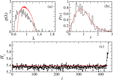
Figure 7: (Colour online) Statistics of spectra of $\mathbf{S}$ obtained from data of sea level pressure. (a) Eigenvalue density for atmospheric pressure data compared against that from random similarity matrix, (b) spacing distribution (histogram) obtained from data and Wigner distribution (solid line), (c) information entropy from data (solid circles) and its RMT average (red line). See text for details.

Now, we consider the sea level atmospheric pressure (SLP) data over the North Atlantic region. This region and in particular this set of data has been well studied in order to understand a pressure see-saw phenomena called the North Atlantic oscillations. In contrast with the elections data in which the political parties (objects) are discrete entities, in this case the SLP values (objects) are continuous. Notice that the formalism requires the objects to be discrete. Hence, we discretise the data as follows. If $a_{max}$ and $a_{min}$ represent the maximum and minimum observed value in the data, we create data intervals of width

$$\Delta=\frac{a_{max}-a_{min}}{p}.$$ (17)

Suppose a data value $a$ lies in, say, 3rd interval $(a_{min}+3\Delta,a_{min}+4\Delta)$, then the discretised data corresponding to $a$ is $3$. In signal processing, this technique of mapping continuous data to a countable set of integers is called quantization [24]. By this process, the entire data set is converted into time series of integers (representing data intervals). Since the observed data in any measurement is known to be contaminated by errors and instrumental noise, it is only fitting that intervals of observed values are analysed instead of the actual values.

We use the NCEP reanalysis data of monthly mean sea level pressure at 434 grid points on the sea surface for the period 1948-2001 [25]. A correlation matrix analysis of this data from the point of view of random matrix theory was reported in Ref. [21]. The data has $N=434$ variables and each variable has time series length of $T=624$. The number of objects (data intervals) is $p=40$. The similarity index $s_{ij}$ in this case measures if the variations of sea level pressure at $i$-th and $j$-th geographical locations are similar. If $s_{ij}=1$, then the discretised data values at these two locations are identical.

Using this discretised data, we compute matrix $\mathbf{S}$ and its spectra. For comparison purposes, we also compute the spectra of its random matrix equivalent $\mathbf{S_{R}}$. Similar to the case of elections data, the eigenvalue density shown in Fig 7(a) (as histogram) displays deviations from that of its random matrix (shown as red curve) at the lower and upper end. These deviating eigenvalues indicate correlations or system specific information that cannot be modelled by randomness assumptions. In this case too, the spacing distribution shown in Fig. 7(b) agrees with the Wigner distribution $P_{W}(s)$. The eigenvectors, corresponding to the deviating eigenvalues in Fig 7(a), also display pronounced deviation from random matrix averages. This is seen in Fig. 7(c) which shows the information entropy as a function of index of eigenvalue. The dominant eigenvectors at the top end of the spectrum are known to capture the pressure patterns that are relevant in atmospheric sciences [21]. We also point out that the components of dominant eigenvector of $\mathbf{S}$, for both elections data and SLP data, have identical phases (not shown here), in agreement with the result shown in Fig. 5(b).

6 Summary

We have studied the problem of computing a measure of similarity for multivariate time series of categorical data, i.e., time series data sets that are not in numerical form. Such data sets are encountered in many situations in social media, say, as response to major events or speeches, in the context of stars or recommendations given to movies or books or other such resources. We construct a similarity matrix $\mathbf{S}$ by assembling together the similarity measure $s_{ij}$ between $i$-th and $j$-th variables. Further, we study the spectra of $\mathbf{S}$ for the case of uncorrelated categorical data and compare with appropriate random matrix results. For most part, the spectra of $\mathbf{S}$ follow random matrix theory prescriptions though the dominant eigenvector deviates due to phase coherence. The eigenvalues and eigenvectors of $\mathbf{S}$ that deviate from random matrix results are seen to signify the presence of correlations that cannot be explained by randomness assumptions that underlie random matrix theory. As an application of this approach, we use the data on the Indian general elections and atmospheric pressure in the North Atlantic ocean region to study the similarity properties. The former is an example which lends itself readily to this analysis but in the latter example the original data is quantized before analysis. Thus, analysis described in this paper can be performed on most of empirically available data sets.

- [1] \NameFriedrich, K. and Blender, R. \REVIEWPhys. Rev. Lett.902003108501.
- [2] \NameLaloux, L. et al. \REVIEWPhys. Rev. Lett.8319991467.
- [3] \NamePlerou, V., et al. \REVIEWPhys. Rev. Lett.8319991471.
- [4] \NamePlerou, V. et al. \REVIEWPhys. Rev. E652002066126.
- [5] \NamePan, R.K., and Sinha S. \REVIEWPhys. Rev. E762007046116.
- [6] \NameSeba, P. \REVIEWPhys. Rev. Lett.912003198104.
- [7] \NameKwapien, J. Drozdz, S. \REVIEWPhys. Rep.5152012115.
- [8] \NameAggarwal, Charu Reddy, Chandan \BookData Clustering : Algorithms and Applications \PublCRC Press \Year2014.
- [9] \NameWarner, R. M., \BookApplied Statistics \PublCambridge Univ. Press \Year2013.
- [10] \NameMehta, M. L. \BookRandom Matrices \Vol142 \PublAcademic Press \Year2004
- [11] \NamePotestio, R., Fabio C. Pierpaolo V. \REVIEWPhys. Rev. Lett.1032009268101.
- [12] \NameVinayak, V., et. al. \REVIEWEurophys. Lett.108201420006.
- [13] \NamePalese, L. L. \REVIEWBiophys. Chem.19620151-9.
- [14] \NameAgresti, A. \BookCategorical Data Analysis \PublWiley-Interscience \Year2007.
- [15] \NameYildirim, M. A., and Michele C. \REVIEWPLoS ONE92014e104813.
- [16] \NameLawson, D. J., Falush, D. \REVIEWAnn. Rev. Genomics. Hum. Gen.132012337.
- [17] \NameTan, P-N., Steinbach, M. Kumar, V. \BookIntroduction to Data Mining. Vol. 1. \PublPearson Addison Wesley, Boston \Year2006.
- [18] \NameLevandowsky, M. Winter, D. \REVIEWNature234197134-35.
- [19] \NameSengupta, A. M. Mitra, Partha P. \REVIEWPhys. Rev. E6019993389.
- [20] \NameHaake, F. \BookQuantum Signatures of Chaos. Vol. 54. \PublSpringer \Year2010.
- [21] \NameSanthanam, M. S. Patra, P. \REVIEWPhys. Rev. E642001016102.
- [22] \NameJones, K. R. W. \REVIEWJ. Phys. A: Math. Gen.231990L1247.
- [23] Data available from http://eci.nic.in/
- [24] \NameGray, R.M. Neuhoff, D. L. \REVIEWIEEE Trans. Inf. Theory.4419982325-2383.
- [25] \NameKalnay, E., et. al. \REVIEWBull. Amer. Meteor. Soc.771996437-470.