Spitzer Survey of Stellar Structure in Galaxies (S⁴G). The Pipeline 4: Multi-component decomposition strategies and data release
(revised 19/11/2014)

Abstract

The Spitzer Survey of Stellar Structure in Galaxies (S⁴G, Sheth et al. 2010) is a deep 3.6 and 4.5 $\mu$m imaging survey of 2352 nearby ($<40$ Mpc) galaxies. We describe the S⁴G data analysis pipeline 4, which is dedicated to 2-dimensional structural surface brightness decompositions of 3.6 $\mu$m images, using GALFIT3.0 (Peng et al. 2010). Besides automatic 1-component Sérsic fits, and 2-component Sérsic bulge + exponential disk fits, we present human supervised multi-component decompositions, which include, when judged appropriate, a central point source, bulge, disk, and bar components. Comparison of the fitted parameters indicates that multi-component models are needed to obtain reliable estimates for the bulge Sérsic index and bulge-to-total light ratio ($B/T$), confirming earlier results (Laurikainen et al. 2007; Gadotti 2008; Weinzirl et al. 2009). In this first paper, we describe the preparations of input data done for decompositions, give examples of our decomposition strategy, and describe the data products released via IRSA and via our web page (www.oulu.fi/astronomy/S4G_PIPELINE4/MAIN). These products include all the input data and decomposition files in electronic form, making it easy to extend the decompositions to suit specific science purposes. We also provide our IDL-based visualization tools (GALFIDL) developed for displaying/running GALFIT-decompositions, as well as our mask editing procedure (MASK_EDIT) used in data preparation. In the second paper we will present a detailed analysis of the bulge, disk, and bar parameter derived from multi-component decompositions.

1 Introduction

How and when did the baryonic mass assemble into galactic disks? How does the fraction of mass confined into bulges evolve over time? How common are galaxies that have no classical bulges, i.e. bulges that have their origin in the early mergers of dark matter halos and baryonic disk systems? These are difficult questions to answer because galaxy evolution involves secular processes such as gas accretion via filaments, where mass presumably ends up in bulges or disks, or internal dynamical evolution, such as the formation of bars which further re-distribute matter in galaxies. Galaxies in the local Universe are the present day manifestations of this evolution and hence provide important clues on the evolutionary processes which took place in the past.

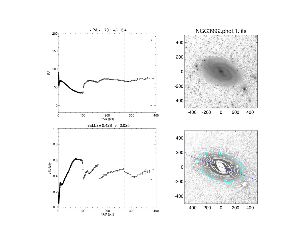
Figure 2: Example of the isophotal profiles derived for NGC 3992 using the IRAF ellipse routine. The plots in the left display the PA and ellipticity profiles versus semimajor axis ($a$) of isophote ellipse: the dashed vertical lines indicate the range used in estimating the outer disk orientation parameters; solid horizontal line indicates the mean over that range. The upper right plot shows the observed, sky subtracted image, clipped at $1.3\times R_{gal}$ (the image region used in decompositions). In the lower right the isophotes are plotted on top of observed (masked) image: the blue isophotes correspond to the $a$ range from which the outer disk orientation ($\epsilon_{outer},PA_{outer}$) was derived; the blue line indicates the assigned $PA_{outer}$. Similar plots for all sample galaxies are available on the P4 web site.

The Spitzer Survey of Stellar Structure in Galaxies (S⁴G, Sheth et al. (2010)) provides an excellent data base with which to measure the stellar mass distribution of galaxies in the local Universe. It is a survey of 2352 galaxies observed in the mid-IR at 3.6 and 4.5 $\mu$m, wavelengths that are largely unaffected by internal extinction (Draine & Lee 1984), and trace mainly the old stellar population (Pahre et al. 2004; however see also Meidt et al. 2012 and Driver et al. 2013), so that the mass-to-luminosity (M/L) ratio in these bands is nearly constant inside the galaxies (Peletier et al. 2012). This is particularly important for deriving the properties of bulges and disks, because dust and star formation are more pronounced in the disks than in the bulges, which in the optical region affect their relative M/L-ratio and thus the relative fraction of the bulge light (Driver et al. 2013). Dust and star formation are significant also in the bulges of late-type galaxies (Fisher 2006; Gadotti 2001). The S⁴G images are deep, reaching azimuthally averaged stellar mass surface densities of $\sim$ 1 M_☉ pc^-2, where the baryonic mass budget at least in spiral and irregular galaxies is typically dominated by atomic gas. S⁴G covers a large range of galaxy magnitudes (over three decades in stellar mass), which makes possible to study both late-type dwarfs and bright galaxies in a uniform manner, and to study when the disk instabilities such as bar formation start to play an important role. Our sample extends to lower galaxy luminosities than most previous samples in which bars have been studied (Barazza et al. 2008; Sheth 2008; Nair et al. 2010; Melvin et al. 2014). Besides galaxy mass, another central factor affecting its structural evolution is its environment (van der Wel 2008; Kormendy & Bender 2012; Weinzirl et al. 2014). S⁴G includes galaxies up to 40 Mpc and covers a wide range of different galaxy environments, including several galaxy groups and the Virgo and Fornax clusters (see Fig. 2 in Sheth et al. 2010).

Plenty of information for the S⁴G sample is already publicly available via the IRSA archive. The data have been processed through Pipeline 1 (Regan et al. 2014) (hereafter P1) which makes mosaics of the observed individual frames, Pipeline 2 (Muñoz–Mateos et al. 2014; P2) which makes masks of the foreground stars and image defects, and Pipeline 3 (Muñoz–Mateos et al. 2014; P3) which measures the basic photometric parameters like the galaxy magnitudes and concentration indices. In Pipeline 4 (P4), described in this study, we decompose the two-dimensional flux distributions of the images into several structural components using GALFIT (Peng et al. 2010). Because even the mid-IR wavelengths are not completely free of such contaminants as hot dust, mass maps are also created for the images in Pipeline 5 (P5, Querejeta et al. 2014). The galaxies in S⁴G have been visually classified at 3.6 $\mu$m by (Buta et al. 2010, 2014), and we use these classifications in the present study. Optical images are also available for the majority of the S⁴G sample (Knapen et al. 2014).

For all of the S⁴G galaxies for which the image quality is good enough (e.g. no superposed bright stars, or image defects), we provide 1-component single Sérsic, 2-component bulge-disk (Sérsic + exponential), and multi-component decompositions, fitting up to four separate structure components. Our main goal is to estimate the parameters of the bulge and the disk in a robust manner, which is the motivation for our decomposition approach. In particular, it is important to include bar-components in the decompositions because the flux of the bar is easily mixed with the flux of the bulge (Laurikainen et al. 2006). Our bulge is defined as a ’photometric bulge’, including the flux in excess of that in disk and bar components; the decompositions themselves do not make assumptions about the physical nature of the bulge, whether a rotation supported classical bulge or a disk star formation/bar vertical buckling related pseudo bulge (see Kormendy & Kennicutt 2004; Athanassoula 2005). To measure the scale lengths and central surface brightness of the disks in a uniform fashion, an exponential function is used whenever possible, instead of a generalized Sérsic function. It is well known that galactic disks can have more than one exponential sub-section (Freeman 1970; Erwin, Beckman & Pohlen 2005). In this study we handle this in a fairly conservative manner: two separate functions (added together) are used to fit the disk in galaxies where distinct inner and outer components of different surface brightness are present, but not in all cases in which a disk break (’truncation’ or ’anti-truncation’) of some degree has been reported in the literature. Our multi-component approach is similar to those used previously by Laurikainen et al. (2005, 2007, 2010), Gadotti (2009), and Weinzirl et al. (2009). Our motivation for offering also the single Sérsic and bulge-disk decompositions is that they are routinely used in large galaxy surveys and high-redshift studies (Häußler 2013; Lackner & Gunn 2012; Cameron et al. 2009; Allen et al. 2006; Driver et al. 2006, 2013). Although single Sérsic fits are not good tracers of the properties of bulges, they are still useful in gross classification of galaxies.

The decomposition results, released via IRSA and our web-page, are given in such a manner that they can be easily extended having different scientific goals in mind. The decompositions were done via GALFIDL, which consists of IDL-based tools for displaying and running GALFIT (see Sect 2.4). It is important to note that due to the large amount of work involved, P4 was started as soon as the first P1 data was available. Because of this we did our own mask editing, and orientation and sky background estimation. These masks form part of the final P2 masks. Due to later changes in P1, part of the images used in P4 contain minor shifts (or differ in size by 1-2 pixels) compared to the finalized P1 images in IRSA. Rather than repeating the time consuming GALFIT decompositions with the updated images, we provide together with the decomposition output files the sky subtracted data and mask images we used.

In this paper, we describe the decomposition method and model components, the preparation of the data for decompositions, and concentrate on illustrating our philosophy behind the construction of the final multi-component decompositions. The results published in tabular form include the outer disk orientation estimates, Sérsic parameters from the 1-component fits, and the final parameters from multi-component decompositions, together with a quality flag for each galaxy. The data products released via IRSA include the GALFIT output files, and all the input fits-files needed for repeating and refining the decompositions. The P4 web pages illustrate the same models in pictorial form, and also provide the GALFIDL code and documentation. (The IRSA products and the P4 web page are described in the two Appendixes). Analysis of the derived bulge, disk, and bar parameters will be presented in paper 2 (Salo et al, in prep.).

2 Decomposition Pipeline

2.1 Decomposition method and model functions

Our decompositions use the GALFIT-software (Peng et al. 2002, 2010), which has become the de facto standard for detailed two-dimensional structural decompositions. It relies on parametric fitting, using the Levenberg-Marquadt algorithm to minimize the weighted residual ${\chi^{2}}_{\nu}$ between observed (OBS) and model (MODEL) images,

$${\chi^{2}}_{\nu}=\frac{1}{N}\sum_{x}\sum_{y}\frac{\left[OBS(x,y)-MODEL(x,y)\right]^{2}}{\sigma(x,y)^{2}}.$$ (1)

The sum is taken over all the used (non-masked) image pixels, and $\sigma(x,y)$ indicates the statistical uncertainty of each pixel (sigma-image). The model image consists of a sum of model components, i.e for bulge, disk, bar etc, convolved with the image Point-Spread Function (PSF-image). Note that the reduced ${\chi^{2}}_{\nu}$ is used, with $N$ denoting the degree of freedom, equal to the number of fitted pixels minus the number of free parameters in the fit.

GALFIT is extremely versatile in its selection of model components. Basically the user defines for each component its ’radial’ profile function, giving the surface brightness $\Sigma(r)$ at each isophotal radial coordinate $r$. The isophotal coordinates are most commonly defined in terms of generalized ellipses (Athanassoula et al. 1990),

$$r(x^{\prime},y^{\prime})=\left(|{x^{\prime}-x_{0}}|^{C+2}+\left|\frac{y^{\prime}-y_{0}}{q}\right|^{C+2}\right)^{\frac{1}{C+2\phantom{{}^{2}}}}.$$ (2)

Here $x_{0},y_{0}$ defines the center of the ellipse, $q=b/a$ is the ratio between minor and major axis lengths. The $x^{\prime},y^{\prime}$ denote coordinates in a system aligned with the ellipse, with the major axis pointing at the position angle $PA$. For pure ellipses $C=0$, while $C>0$ indicates boxy and $C<0$ disky isophotes. For the pipeline decompositions, simple elliptical isophotes $C=0$ are used for all components. Besides generalized ellipses, GALFIT provides several alternatives, such as definition of isophotal shape via azimuthal or bending modes, or via coordinate rotations, which would form a natural basis for detailed modeling of e.g. logarithmic spirals. To keep our models relatively simple (and uniform over the wide range of angular sizes and surface brightnesses spanned by the sample), we have not used these advanced GALFIT features. Keeping the models simple makes the interpretation of the observation minus model residuals more straightforward (see the NGC 1097 examples in Sheth et al. (2010)).

The pipeline decompositions use five different choices for the model components/radial functions:

1) The bulge component is described with a Sérsic profile (“sersic”)

$$\Sigma(r)=\Sigma_{e}\exp\left(-\kappa\left[(r/R_{e})^{1/n}-1\right]\right),$$ (3)

where $\Sigma_{e}$ is the surface brightness at the effective radius $R_{e}$ (isophotal radius encompassing half of the total flux of the component). The Sérsic-index $n$ describes the shape of the radial profile, which becomes steeper with increasing $n$. In particular, $n=1$ corresponds to an exponential profile and $n=4$ to a de Vaucouleurs profile. The factor $\kappa$ is a normalization constant determined by $n$. In GALFIT the corresponding “sersic”-function is used, with the integrated magnitude $m_{bulge}$ as a free parameter (instead of $\Sigma_{e}$).

2) In the case of low or moderate inclination, the disk component is described with an infinitesimally thin exponential disk (“expdisk”) ,

$$\Sigma(r)=\Sigma_{o}q^{-1}\exp(-r/h_{r}),$$ (4)

where $\Sigma_{o}$ is the central surface brightness of the disk observed from the perpendicular direction and $h_{r}$ denotes the exponential scale length. In this case the $q=\cos i$, where $i$ is the disk inclination. Assuming no extinction, $\Sigma_{o}q^{-1}$ is the projected surface brightness at the sky plane. The “expdisk”-function in GALFIT is used, with integrated $m_{disk}=-2.5\log_{10}(2\pi\Sigma_{0}\ {h_{r}}^{2})$ as a free parameter (instead of $\Sigma_{0}$). Note that in cases that had more than one disk component, the inner disk was sometimes fit with a sersic or ferrer2 function, to allow the profile to drop faster than with expdisk.

3) For a nearly edge-on disk (apparent axial ratio $q\lesssim 0.2$), the function (“edgedisk”)

$$\Sigma(r_{x},r_{z})=\Sigma_{o}\frac{r_{x}}{h_{r}}K_{1}\left(\frac{r_{x}}{h_{r}}\right)\ {\rm sech}^{2}(r_{z}/h_{z}),$$ (5)

is adopted, where $r_{x}$ and $r_{z}$ are the (positive) distances along and perpendicular to the apparent major axis of the disk, and $K_{1}$ stands for a modified Bessel function. This function corresponds to the line-of-sight (viewing along the disk plane) integrated surface brightness of a 3D luminosity density distribution (van der Kruit & Searle 1981)

$$L(r_{x},r_{z})=\frac{\Sigma_{0}}{2h_{r}}\exp(-r_{x}/h_{r})\ {\rm sech}^{2}(r_{z}/h_{z}).$$ (6)

4) For a bar component a modified Ferrers profile (“ferrer2”) is assumed,

$$\Sigma(r)=\left\{\begin{array}[]{ll}\Sigma_{o}\left[1-(r/r_{out})^{2-\beta}\right]^{\alpha}&r<r_{out}\\ 0&r\geq r_{out}\end{array}\right.$$ (7)

Here $r_{out}$ defines the outer cut of the profile, while $\alpha$ defines the sharpness of this cut. The parameter $\beta$ defines the central slope of the profile, and $\Sigma_{0}$ is the central surface brightness (in the plane of the sky).

5) When the galaxy contains an unresolved central component it is fit with a PSF-convolved point source (“psf”). In this case the free parameter is the total magnitude $m_{psf}$. Typically this component, if present, is not an active or starburst nucleus, but rather a small bulge with angular size so small that it cannot be resolved in the S⁴G images ($R_{e}\lesssim FWHM=2.1\arcsec$ of S⁴G images).

For the decomposition pipeline we chose to do three types of decompositions: 1) one-component Sérsic-fits, 2) two-component bulge-disk decompositions using Sérsic-bulges and exponential disks (or edge-on disk if appropriate), and 3) multi-component ’final’ decompositions, optionally with additional bar, disk and central components (the level of complexity of the models is discussed in more detail in Section 3). The first two types of models are made in an automatic manner, while the final models always include human judgment about what components should be included.

2.2 Preparation of data for decompositions

2.2.1 What is needed?

The S⁴G data analysis Pipeline P1 (Regan et al. 2014) provides image mosaics in both 3.6 and 4.5 $\mu$m, accompanied with weight-images, which indicate for each pixel location the number of original frames covering it. Together with the header information, these weight images provide the means for producing the sigma-images used in GALFIT.

Before decompositions can be started, frames masking the foreground/background objects and various image defects are needed. Additionally we need the galaxy centers, sky background values, and the orientation of the galaxy relative to the sky plane, estimated from the shape of the galaxy’s outer isophotes. In principle, this additional input for decompositions are published for all S⁴G galaxies in Muñoz–Mateos et al. 2014, available via IRSA/S⁴G Pipeline 3. However, at the time our Pipeline 4 decompositions were made, these data was not yet available. Therefore, we made our own sky background estimates and ellipse fits. Also, the automatically created masks (see Muñoz–Mateos et al. 2014) were visually inspected and hand-edited when needed (these edited masks later became part of the final S⁴G masks). If the decompositions are rerun starting from the output files provided in P4, it is important to use the data and mask images, as well as the pre-defined parameters offered via P4.

In summary, Pipeline 4 consists of scripts for editing the masks, determining the galaxy centers, estimating the sky background, fitting isophotal ellipses, preparing the input files, and running GALFIT. It also includes tools for visualization of the GALFIT output files (see Sect 2.4) and routines for storing the data on IRSA server (Appendix A) and the P4 web pages (Appendix B).

2.2.2 Mask images

The raw masks for the S⁴G 3.6 $\mu$m images were made in P2 with the SExtractor software (Bertin & Arnouts 1996), as described in Muñoz–Mateos et al. (2014). Various automatic detection thresholds for point sources were used. However, it soon became evident that no single criterion was sufficient to exclude all extra sources, without sometimes affecting also the galaxy light itself, in which case the masks needed manual editing. Also, in some cases the images contained artifacts that needed to be removed by hand. To speed-up this editing process, we developed a small portable IDL-routine (MASK_EDIT). Basically it displays on the screen simultaneously the original and masked images, and allows the user to remove/insert masked regions interactively. As an initial step of P4, all of the raw 3.6 $\mu$m masks were visually checked and edited if needed. The resulting masks are suitable for the purposes of our structural decompositions. However, because the wings of the PSF are quite extended (see Section 2.2.6) more extensive masking might be required in some applications. The MASK_EDIT routine, with source code and examples of use, is available at the P4 web page.

2.2.3 Galaxy centers, sky background, isophotal profiles

After the edited masks were completed, we run the galaxies through a semi-automatic IDL script which determines the galaxy centers, sky background levels and galaxy orientation parameters. The accurate galaxy center is measured with the cntrd-routine, after its approximate location is interactively defined. We also have the option to mark the center by force, in case the automatic center finding routine does not work satisfactorily even after repeated trials.

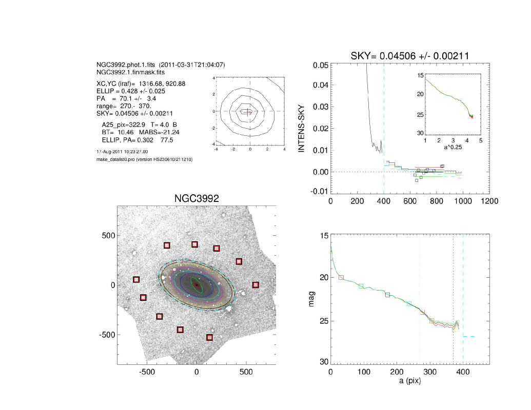
Figure 1: Example of the determination of sky background for NGC 3992. The small upper left frame illustrates the center location found with cntrd-routine (black cross) relative to the image isophotes near the center (dashed red lines indicate the nearest integer pixels). In the lower left frame, red boxes indicate the local regions used for estimating the sky background: the mean and the RMS of these local median values were adopted for the sky background and its uncertainty (SKY and DSKY, respectively). The dashed ellipse indicates the visually estimated galaxy size ($R_{gal}$). The white specks indicate masked stars. The upper right frame shows the intensity profile after subtracting the SKY value (indicated in the title of the plot; note the linear scale, intensities are from IRAF ellipse fits), marking also the $\pm DSKY$ (vertical red/green lines) and the median sky values in local measurement regions (boxes). The vertical dashed line corresponds to $R_{gal}$ The insert shows the same profile, but as magnitude versus $a^{0.25}$, where $a$ is the isophotal major-axis distance: a de Vaucouleurs profile would appear a straight line in this plot. The lower right frame shows the intensity profile in magnitude units (AB-magnitudes): red/green profiles correspond to adding/subtracting DSKY to the sky background. All distances are in pixels ($0.75\arcsec$). Similar plots for all sample galaxies are given on the P4 web site.

The regions used for estimation of the sky background are identified manually, by selecting several (typically 10-20) locations outside the visible galaxy, while avoiding the image edges or contaminated areas. The local sky values in these locations are obtained by taking medians of the non-masked pixels in 40 pix $\times$ 40 pix boxes. The global sky background (SKY) and its uncertainty (DSKY) are then estimated from the mean and standard deviation of these local values, respectively (see Fig. 1). In section 4, using the estimated DSKY, we show that the expected uncertainty of decomposition parameters caused by possible uncertainties in background subtraction is negligible. We also determine the average RMS sky variation, by taking the median of standard deviations in different sky regions (after removing outliers by iterative 3-sigma clipping). We use the sky RMS estimates in Section 2.2.5 for assessing the validity of theoretically calculated sigma-images.

We calculate the isophotal profiles with a pyraf script called from IDL, using the standard IRAF ellipse algorithm (Jedrzejewski 1987). As inputs for the ellipse fitting the sky background subtracted data image and the edited mask image are used. We fix the ellipse center to the previously found galaxy center and use a logarithmic increment of 0.02 between isophote levels. As often happens with IRAF ellipse, the fit does not necessarily converge over the whole galaxy area: we have an option to re-try the fit with different starting locations until a successful fit is obtained over the whole galaxy region (see Fig. 2). From the isophotal profiles, we choose a semi-major axis range from which outer orientations ($(b/a)_{outer}=1-\epsilon_{outer},PA_{outer}$) are estimated. Also, a rough estimate of the galaxy outer radius, $R_{gal}$, is made to define the image region used in the GALFIT decomposition.

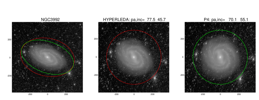
Figure 3: Example of deprojections with HyperLeda and P4 orientation parameters ($(b/a)_{outer}$ and $PA_{outer}$) for NGC 3992. The red and green ellipses on the original image in the left illustrate the HyperLeda and P4 parameters, respectively (semimajor axis of the ellipse equals $R_{gal}$), the frame in the middle shows the deprojection with HyperLeda orientation, and that in the right with P4 parameters: here the inclination is taken simply as $i=\cos^{-1}(b/a)$ (note that this differs from the inclination (“incl”) listed in HyperLeda, which includes a morphological type-dependent correction for the assumed disk thickness). Clearly, the face-on disk is closer to axisymmetric when using P4 parameters: the difference would remain if the thickness-corrected HyperLeda inclination were used (47 degrees for this example). Similar plots for all sample galaxies can be found in the P4 web site.

Figures 1 and 2 give examples of typical plots produced during these preparatory steps, illustrating the sky background fitting and the elliptical isophote profiles. The estimated $\epsilon_{outer}$ and $PA_{outer}$ are marked. In all our decompositions, we fix the orientation of the disk component to these outer values and interpret them to represent the galaxy viewing inclination. Therefore, extra care is taken to estimate the orientations reliably. For example, the corresponding inclination $i_{disk}=\cos^{-1}(b/a)_{outer}$ is visually checked by de-projecting the galaxy images to face-on. Figure 3 shows an example of such a de-projection, also comparing the estimated inclinations with those calculated from axial ratios given in the HyperLeda database. Typically, our $(b/a)_{outer}$ and $PA_{outer}$ are determined at much lower surface brightness levels than those in HyperLeda (which are mainly from RC3 de Vaucouleurs et al. (1991)). P4 values are thus less affected by bulges, bars, or prominent spirals, and should reflect better the orientation of the underlying extended disk, which appears with circular outer isophotes in face-on projection. In some cases, S⁴G images are so deep that the outermost isophotes are dominated by an outer stellar halo rather than the disk. Good examples are NGC 681, NGC 1055 and NGC 4594. Possible misinterpretations of the outer isophotes were avoided by visually inspecting all the images: when the disk (identified with spiral arms, rings, and lenses) is clearly more inclined than suggested by the outermost isophotes of the image, the isophotes in the disk region were used for the estimate of galaxy orientation. For nearly face-on galaxies, the possible stellar halos are more difficult to distinguish, but in these cases the involved error in the orientation is less important. The final P4 axial ratios and position angles, center locations, and sky background values are listed in Table I. For each galaxy we also include a flag indicating the inclination uncertainty: ’ok’ indicates that outer isophote axial ratio should give a reliable estimate of $i_{disk}$, ’u’ indicates that the inclination is uncertain, while ’z’ indicates that the galaxy is close to edge-on (the axial ratio is not used for an inclination estimate).

A scatter plot of P4 axial ratios versus HyperLeda values is presented in Fig. 4 (upper left frame; only galaxies with flag=’ok’ are shown). As anticipated, the P4 axial ratios are on the average closer to unity than those in HyperLeda, though the difference is not very large (median $(b/a)_{P4}-(b/a)_{HyperLeda}=0.024$). On the other hand the standard deviation of the difference is quite large ($\sim 0.1$). The upper right frame makes a similar comparison to P3 axial ratios (Muñoz–Mateos et al. 2014) which correspond to a fixed surface brightness level $\mu_{3.6}=25.5$ mag/arcsec². On average, P4 orientations are measured at about 0.9 times this distance. The scatter is now significantly reduced and no systematic difference is seen between P3 and P4. The lower frames in Fig. 4 compares the position angles (now also ’z’ galaxies are included). In general the differences between P4 and HyperLeda are fairly small: for $b/a<0.8$ the median absolute difference is $2^{\circ}$. The difference between P4 and P3 is even smaller (median absolute difference $0.9^{\circ}$ for $b/a<0.8$). Nevertheless there are some exceptions, most notably NGC4594 (The Sombrero Galaxy): in this case the P3 fixed isophote orientation corresponds to the extended halo, while the P4 orientation refers to the edge-on disk.

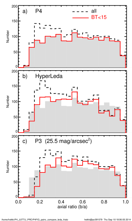
Figure 5: Distribution of axial ratios, calculated with P4 (a), HyperLeda (b), and P3 orientation parameters. Hubble types $T\leq-4$ and $T>10$ are excluded (using Buta et al. 2014 Mid-IR classification). Dashed line indicates the whole S⁴G sample, with the magnitude selection $BT_{corr}<15.5$, where $BT_{corr}$ is the inclination-corrected blue magnitude from HyperLeda. Solid line corresponds to a similar limit, but using non-corrected blue magnitude $BT$. To ease the comparison the P4 histogram for $BT<15$ is shown as the shaded region in each frame.

Since we are fixing the disk orientations in the decompositions it is important to check the consistency of our inclinations. Figure 5a displays the histogram of the P4 axial ratios for Hubble types $-3\leq T\leq 10$. In case of a randomly oriented sample of thin disks, the distribution of $b/a$ should be flat. In case of finite vertical thickness a drop would be expected near a lower limit $b/a=q_{i}$, where $q_{i}$ is the intrinsic aspect ratio of the galaxies. According to Fig. 5a such a drop is evident for $b/a\lesssim 0.15$. However, overall the sample contains an excess number of galaxies with small axial ratios $b/a\lesssim 0.5$ (see the dashed line in Fig. 5a). Similar trend is seen also when using the HyperLeda axial ratios (Fig. 5b) or P3 isophotal orientations (Fig. 5c). A possible explanation for the excess of small $b/a$ ratios is that the S⁴G sample has been selected (Sheth et al. 2010) using an inclination-corrected blue magnitude limit ($BT_{corr}=15.5$): if this dust correction were exaggerated, say for very late types, it would lead to an excess of faint, highly-inclined galaxies. This explanation is supported by the solid curves in Fig. 5 which display the histograms when limiting to galaxies with non-corrected $BT<15$: now the histogram of P4 values is quite flat. The histogram for P3 isophotal axial ratios is rather similar, though there are somewhat fewer small $b/a\lesssim 0.2$ values. This could be due to the above-mentioned faint stellar halos: in case of nearly edge-on galaxies a fixed surface brightness level could pick up the rounder faint outer envelopes, whereas in P4 we have in such cases tried to trace the disk isophotes. On the other hand, compared to both P3 and P4, the HyperLeda distribution has a clear deficit of large axial ratios, mostly likely due to the influence of inner non-axisymmetric structures.

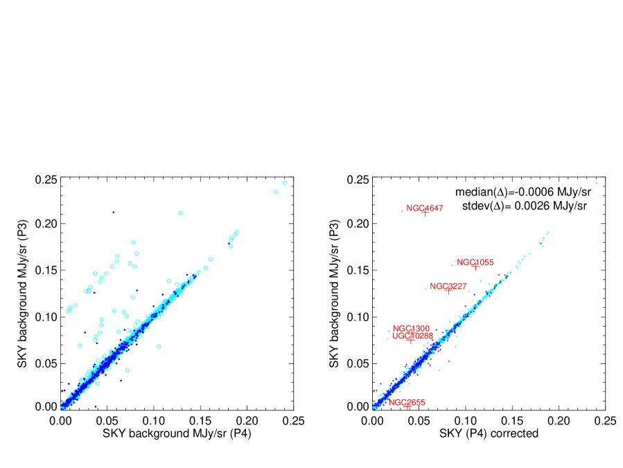
Figure 6: The left frame displays the used P4 sky background estimates (SKY) in comparison to P3 (Muñoz–Mateos et al. 2014; their variable ’SKY1’). The large apparent differences are due to use of different versions of P1 mosaics. In the right we have corrected the P4 values to corresponds to the final P1 mosaics (=those used in P3). Excluding the few deviant cases (discussed in the text) the median difference between P3 and P4 is 0.003 MJy/sr. Light and dark blue symbols indicate observations during cryogenic and warm Spitzer missions, respectively.

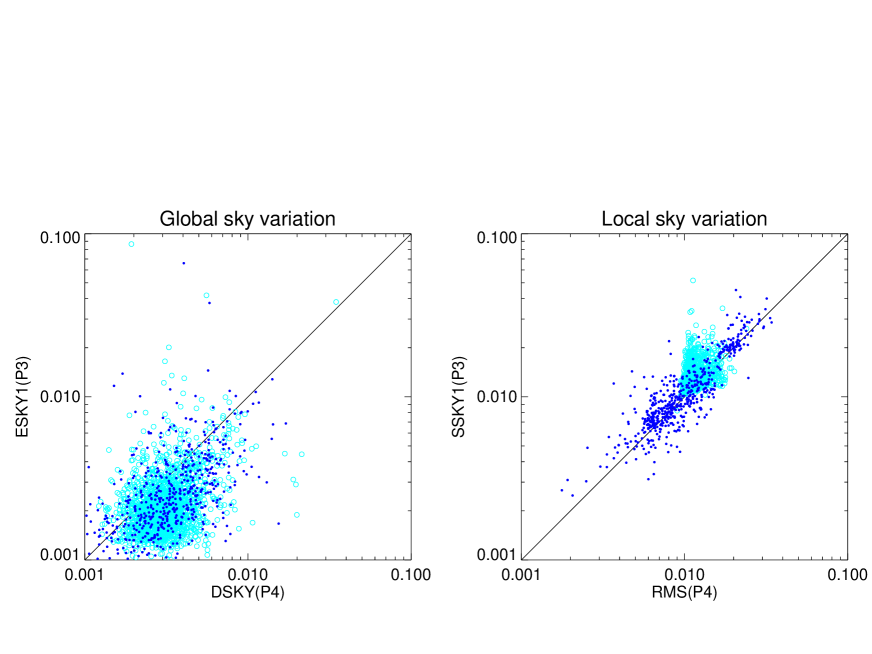
Figure 7: Comparison of P4 and P3 sky variation estimates. The left frame displays the global variations, estimated from the standard deviation of sky measurements at different areas (variable ’DSKY’ in P4 and ’ESKY1’ in P3; the symbol colors are the same as in the previous Figure). In the right the local variation, estimated from the median scatter of sky values in local measurement areas (variable ’RMS’ in P4 and ’SSKY1’ in P3).

It is interesting to compare our sky background estimates to those in P3. In P3 an automatic sky measurement is made using 45 sky regions with 1000 pixels each. The regions are chosen close to the distance $2R_{25}$ from the galaxy center ($R_{25}$ is the blue band 25 mag isophotal radius from HyperLeda; if needed the distance of sky regions is modified manually). According to Fig. 6 there is a very good agreement in the estimated sky backgrounds between P3 and P4 (see the right frame which takes into account that different P1 mosaics are used for some of the galaxies). This good agreement is remarkable as the measurements are made completely independently and with different methods. The median difference between the sky determinations (0.0006 MJy/sr) is only about 1% of the typical sky background value, and its standard deviation (0.003 MJy/sr or ) is comparable to the magnitude of global sky variations in both sets of estimates (see Fig. 7). However, Fig. 6 also reveals some cases where the difference between P4 and P3 is significant: inspection of the images indicates that this is due to a bright star (NGC1055), a nearby interacting component (NGC3327, NGC4647), or a too small FOV (NGC2655). In two cases (NGC1300, UGC10288) the final P1 mosaic used by P3 is much improved over the earlier version used in P4.

Fig. 7 compares our sky background variation estimates (’DSKY’ denotes global variations between sky measurement regions and ’RMS’ the average of the locally determined rms-scatter) with the corresponding estimates in P3 (Muñoz–Mateos et al. 2014; their parameters ESKY1 and SSKY1, respectively). There is a good overall agreement in the level of estimated global variation (left frame): the somewhat larger values for P4 are likely to follow from the larger range of radii we used for the sky measurement regions compared to P3. Also the local sky rms values show good agreement (right frame).

2.2.4 Input data images

As input for the GALFIT decompositions we use the 3.6 $\mu$m images. Because all necessary data reduction and calibration were already done in P1, the main preparatory steps are to subtract the estimated sky background value and determine which image region to include in the decomposition. In principle, GALFIT can also fit the sky background. However, this requires that the decomposed image region contains sufficiently large regions free of galaxy light or other contaminants. Use of such large image regions would slow down the decompositions considerably. Even more importantly, the S⁴G images often fill a substantial part of the raw frames or there are sudden jumps in the background levels (well outside the galaxy). To have a control of where the sky level is estimated, we chose to do the sky background evaluation manually, as described in Sect. 2.2.3, and to limit the decomposition to the rectangular region $\pm R_{fit}$ around the galaxy center. In practice, we choose $R_{fit}=1.3\times R_{gal}$, where $R_{gal}$ is our visually estimated outer size of the galaxy. Finally, the image header keyword EXPTIME is set to 1 sec (as a default GALFIT will normalize the input data values with EXPTIME, which keyword is not relevant for P1 mosaics), and all NaN’s (bad image values indicated with Not-a-Number value) are replaced with a constant value, and flagged in the mask in order to prevent them from affecting the decompositions.

2.2.5 Sigma-images

The sigma-images quantify the statistical uncertainty of each image pixel and thereby determine the weights applied in GALFIT decompositions. This uncertainty contains two contributions: the noise contribution associated with the number of photons arriving at the instrument (’photon noise’ or ’shot noise’), and the noise originating from the instrument itself. The photon noise is assumed to follow a Poisson distribution, and it arises from two sources, the flux associated with the galaxy light and the flux coming from the sky background (zodiacal light). The main concern in the construction of the sigma-images is that the relative contributions of the photon noise and the instrumental noise are correctly estimated, so that correct relative weights are used in the decomposition for the bright central regions of the galaxies and for their faint outskirts.

The sigma-images are calculated using the pixel values and header information in the 3.6 $\mu$m data images and the pixel values of the weight images. The images provided by P1 are in flux units (MJy/sr), and for the calculation of the noise their pixel values $F$ are converted to the number of electrons $N_{e}$,

$$N_{e}=\frac{F+F_{bg}}{F_{conv}}~{}\times T_{frame}\times N_{frames}\times g,$$ (8)

where $F_{bg}$ is the zodiacal light background which has been subtracted from the frame prior P1 by the automatic Spitzer pipeline (its value is given by the header keyword SKYDRKZB). Note that the flux $F$ contains besides the galaxy light also the sky background which has been subtracted in P4, $F=F_{gal}+F_{sky}$. The $F_{conv}$ is the conversion factor between flux units and original digital units (header keyword FLUXCONV, in units of MJy/sr per DN/sec), $T_{frame}$ is the integration time/frame in seconds, $N_{frames}$ is the number of combined frames for each pixel, and $g$ is the detector gain factor (GAIN in units of e/DN). The number of frames combined is coded to the pixel values $W$ of the weight images, $N_{frames}=W/10$. Note that $T_{frame}=30$ sec must be used instead of the original integration time/frame given by the header keyword FRAMTIME: this is because during the compilation of P1 mosaics the pixel values have been normalized to this value regardless of the original $T_{frame}$. The statistical uncertainty of $N_{e}$ in each pixel is then calculated as a combination of Poisson noise (photon noise) and the readout noise of the detector (RON),

$$\sigma^{2}(N_{e})=N_{e}+N_{frames}\times RON^{2}.$$ (9)

We use RON = 15.0, 14.6, and 21 electrons, for FRAMTIME = 12, 30, and 100 secs, respectively. Note that these values, communicated by the Spitzer Science Center Helpdesk, deviate slightly from those given by the image header keyword RONOISE. The $\sigma(N_{e})$ is then converted to the estimated uncertainty of the image flux (note that $\sigma(F_{gal})$ equals $\sigma(F)$ since $F_{sky}$ is constant)

$$\sigma_{est}(F)=\sigma(N_{e})\times F_{conv}/(T_{frame}\times N_{frames}\times g).$$ (10)

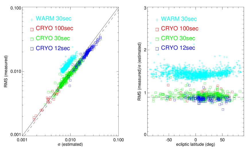
Figure 8: Comparison of measured and theoretical $\sigma$. The left frame displays the measured RMS in sky regions against the estimated $\sigma$, which takes into account the read-out noise, and the Poisson noise due to sky background (including the zodiacal light contribution removed by the automatic Spitzer pipeline). For the cryogenic mission phase the agreement is fairly good, with $RMS\approx 0.9\ \sigma_{est}$ (indicated by the dashed line; solid line indicates a one-to-one correspondence). For the warm phase the observed RMS is about 50% larger than the theoretically estimated noise. The right frame shows the ratio of the observed and estimated noise as a function of ecliptic latitude.

In order to assess the validity of this estimate we compare it to the actual noise measured directly from the image. In Fig. 8 this is done for the sky measurement regions. In the left frame the measured sky RMS (an average over all sky determination boxes) is plotted against the estimated $\sigma_{est}$ from Eq. 10. Colors distinguish between archival images from the cryogenic mission phase (original exposure time/frame either 12, 30, or 100 secs) and the new observations during the warm Spitzer mission (time/frame 30 secs, with the total exposure time of 240 seconds). For the archive images the overall agreement is quite good: there is a practically linear trend $RMS\approx 0.9\ \sigma_{est}$ holding for all three frame times, with the largest noise levels corresponding to the shortest frame times which have the largest contribution from the readout noise. The factor $\sim$ 0.9 is probably due to the P1 mosaicking process, during which the images have been combined and sampled to 0.75 ″pixel size from the native pixel size of 1.2 ″. Because of this sampling the adjacent pixel values are strongly correlated, which is not taken into account in our theoretical estimate. Instead of trying to account in detail for the noise propagation during the mosaicking process we apply an empirical correction

$$\sigma_{decomp}(F)=0.9\ \sigma_{est}(F)\ \ \ \ \ {\rm(cryogenic\ mission)}$$ (11)

to be used in decompositions of cryogenic phase archival images.

In contrast, for the warm mission the observed RMS is nearly 50% larger than the theoretical estimate (Fig. 8), indicating the presence of an additional source of noise. Also, there is a noticeable drop in $RMS/\sigma_{est}$ ratio near the ecliptic plane (not present in the data from the cryogenic phase), indicating that the photon noise contribution to the $\sigma_{est}$ (largest at $l\approx 0^{\circ}$) is overestimated compared to the instrumental contribution (constant with $l$). Following the advice of Spitzer Science Center Helpdesk, we include an additional instrumental noise component ($\sigma_{conf}$), which is added quadratically to the theoretical noise estimate. To account for the P1 mosaicking process, the multiplicative factor of 0.9 is again included. We thus adopt

$$\sigma_{decomp}(F)=0.9\ \sqrt{{\sigma^{2}}_{est}(F)+\sigma_{conf}^{2}}\ \ \ \ \ {\rm(warm\ mission)}$$ (12)

for the warm mission images. The value of the empirical correction term $\sigma_{conf}^{2}$ is estimated by this formula when applied to the sky measurement regions; the same formula is then applied to all image pixels. The adopted values of $\sigma_{conf}$ are listed in Table I above.

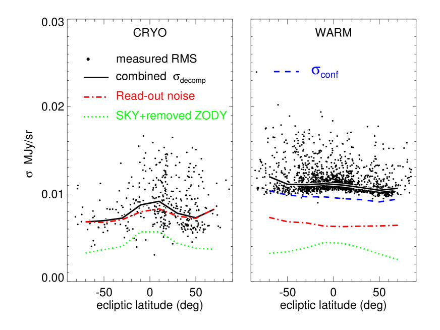
Figure 9: Different contributions to the sky background noise. The symbols indicate the measured average noise in sky measurement regions (RMS) in the cryogenic mission archival images (left frame; for clarity only those with 30 sec original frame time are shown) and in warm mission images (right frame), as a function of ecliptic latitude. The lines indicate various noise contributions and the total noise calculated with Eqs. (11) and (12): for clarity a mean over 20 deg bins is shown. Note that in the left frame the peaking of readout noise contribution close to ecliptic plane is just a spurious effect.

Figure 9 illustrates the magnitudes of different contributions to the sky background noise. For the archival images (cryogenic phase, left frame) the noise is dominated by the readout-noise, though the Poisson contribution due to zodiacal light (the $F_{sky}$ we have subtracted in P4 + the SKYDRKZB subtracted during automatic Spitzer pipeline) still has a noticeable contribution. For the warm Spitzer mission (right frame) the extra noise term is even larger than the readout contribution.

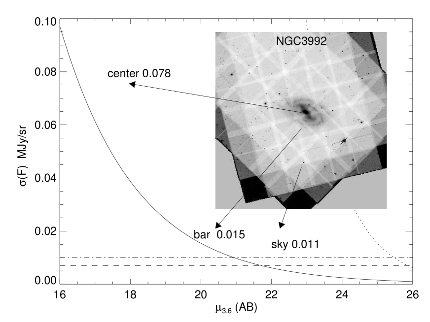
Figure 10: Comparison of galaxy flux and background noise contributions. The solid curve is the calculated Poisson noise associated with the galaxy flux $F_{gal}$, as a function of surface brightness (in 3.6 micron AB magnitudes; $F_{gal}$ is converted to surface brightness with Eq. 13). The horizontal lines indicate the typical background noise levels for the warm and cryogenic mission phases (dot-dashed and dotted lines, respectively; they include both the noise associated with sky background flux and instrumental contributions). The insert shows the $sigma$-map for NGC 3992. The structure in the background is due to different number of frames covering each pixel. Also notice how the galaxy stands out clearly on the $sigma$-map. The dotted line crossing the horizontal lines at $\mu_{3.6}\approx 25.5$ indicates the galaxy flux in MJy/sr.

Nevertheless, at the central parts of the galaxies the photon noise associated with the galaxy light $F_{gal}$ is the largest source of noise. This is illustrated in Fig. 10) which compares the Poisson and background contributions as a function of surface brightness. The two horizontal lines indicate the typical background noise levels for the cryogenic (lower) and warm (upper) phases (includes both instrumental and noise due zodiacal light). The inset figure illustrates how the $\sigma$-map looks for the galaxy NGC3992 (observed during the warm mission). Near the center ($\mu\approx 17$), the photon noise due to $F_{gal}$ completely dominates, though already in the bar region ($\mu=20-21)$ both photon and instrumental contributions are important. Altogether the sigma-images and thus the applied relative weights between galaxy and background regions are intermediate between those typically encountered when decomposing ground-based optical and NIR-images. In the former case the photon noise due galaxy light usually dominates, while in the latter case the sigma-image is almost completely dominated by the background noise, so that the weight is almost constant for all pixels (this applies e.g. to Janz et al. 2014 GALFIT decompositions of Virgo dEs based on ground-based H-band images).

In principle, the obtained $\sigma_{decomp}$ is just a statistical estimate of the true underlying variance at each pixel. We did some experimentation by smoothing the sigma -images (median averaging with kernels amounting up to 20 pixels). Except in the case of a few galaxies with very centrally peaked light profiles, this smoothing had very little influence on the final decomposition parameters. For the galaxies where smoothing played a role, the derived parameters were in any case uncertain (for example, the bulge Sérsic index obtained unrealistically high values $>$ 10). In the end, we decided to apply no smoothing at all. Tests related to the sigma-images are presented in Section 4.3.

2.2.6 PSF-image

The IRAC data is not very well sampled: its native pixel resolution is 1.2″, which is close to the Gaussian spread of a point source observed at channel 1. As discussed in detail in Peng et al. (2010), in such a case an oversampled PSF should be used. The IRAC PSF has also wide wings (see Fig. 11), so that a relatively large convolution box size must be used in decompositions: we set this to $40\arcsec\times 40\arcsec$ (in some cases with a very centrally peaked light profile this region was extended to $150\arcsec\times 150\arcsec$ with considerable increase in CPU time). Note also that IRAC PSF depends slightly on the instrument orientation. Therefore, in principle a separate PSF should be used with each image, determined from point sources in the same frame, or a combination of appropriate PSFs, in case the final image is a combination of several images obtained at different times. Clearly, such a procedure would be very time consuming. Fortunately, such an accuracy is hardly needed in our decompositions. The common oversampled PSF provided by T. Jarrett was used for all images, made as a composite over several instrument rotation angles. Fig. 11 displays the PSF, as well as a Gaussian profile (with $FWHM=2.1\arcsec$) approximately matching the core of the composite PSF. Also shown is an azimuthally averaged profile of the composite PSF. It will be shown in Section 2.5 that it is important to account for the central core, as well as for the nearly circular wings of the PSF, whereas the outermost spikes have less importance for the obtained decomposition parameters.

Table 1: Pipeline 4 parameters: galaxy center, outer orientation, and sky background

IDE		xc	yc	PA $\pm$ dPA	ELL $\pm$ dELL	RANGE	FLAG	SKY	DSKY	RMS	$\sigma_{conf}$
ESO011-005		780.84	299.02	42.7 $\pm$0.1	0.747 $\pm$0.002	13 - 16	z	0.0125	0.0039	0.0109	0.0092
ESO012-010		760.68	294.95	146.2 $\pm$1.1	0.542 $\pm$0.012	75 - 90	ok	-0.0022	0.0025	0.0109	0.0096
ESO012-014		782.57	459.99	31.0 $\pm$5.2	0.580 $\pm$0.040	67 - 75	u	0.0080	0.0033	0.0106	0.0091
ESO013-016		478.49	282.78	-14.3 $\pm$3.1	0.343 $\pm$0.031	52 - 82	ok	0.0041	0.0027	0.0101	0.0084
ESO015-001		291.43	294.80	125.7 $\pm$2.7	0.586 $\pm$0.018	56 - 75	u	0.0050	0.0018	0.0102	0.0086
ESO026-001		795.50	495.47	19.3 $\pm$21.1	0.060 $\pm$0.028	52 - 60	ok	0.0125	0.0024	0.0105	0.0091
ESO027-001		776.34	294.63	12.5 $\pm$10.1	0.216 $\pm$0.061	112 - 127	u	0.0109	0.0032	0.0112	0.0097
…
UGC12791		295.88	289.63	82.6 $\pm$1.4	0.709 $\pm$0.037	45 - 60	ok	0.0406	0.0033	0.0110	0.0094
UGC12843		290.20	287.90	17.5 $\pm$3.9	0.553 $\pm$0.058	52 - 67	u	0.0418	0.0037	0.0105	0.0086
UGC12846		571.15	851.20	-4.7 $\pm$14.0	0.127 $\pm$0.031	60 - 67	u	0.0446	0.0007	0.0019	0.0000
UGC12856		291.07	296.89	16.9 $\pm$1.5	0.615 $\pm$0.049	48 - 75	u	0.0401	0.0025	0.0111	0.0099
UGC12857		284.91	280.12	33.5 $\pm$0.2	0.760 $\pm$0.009	15 - 30	z	0.0453	0.0018	0.0110	0.0096
UGC12893		294.93	283.15	87.2 $\pm$3.8	0.131 $\pm$0.039	52 - 67	ok	0.0463	0.0022	0.0110	0.0093

Note. — Galaxy center $x_{c},y_{c}$ is given in pixels, ELL $\pm$ dELL and PA $\pm$dPA are the outer isophote ellipicity and position angle together with their standard deviations in the measurement range, given by RANGE (in arcsecs). FLAG indicates whether the inclination can be reliably estimated from the ellipticity ($i_{disk}=\cos^{-1}(1-\epsilon_{outer}))$: ok = reliable, u = uncertain, z= nearly edge-on galaxy. SKY, DSKY, and RMS give the estimated sky level and its global and local variation (in MJy/sr). The last column $\sigma_{conf}$ gives the estimated extra instrumental noise component during the Spitzer warm mission (See Sect 2.2.5).

The Figure + caption modfied according to referee’s suggestion

Figure 4: Comparison of outer disk orientation parameters to those in HyperLeda, and to the P3 orientation parameters corresponding to fixed $\mu_{3.6}=25.5$ mag/arcsec² isophote. In the upper row axial ratios are compared: the green line indicates the running median of HyperLeda (or P3) axial ratio, calculated in bins of 100 galaxies; gray indicates the RMS scatter in the bin. Red line indicates unit slope. The labels give the median difference and rms of the difference compared to P4: P4 axial ratios are generally larger than those in HyperLeda while the difference to P3 is small. The lower frames displays the absolute difference in the position angles: squares mark deviant points with $|\Delta PA|>15^{\circ}$ for $b/a<0.5$. In the upper frames only galaxies with orientation uncertainty flag ’ok’ are included, while in the lower frames also galaxies with flag ’z’ are included.

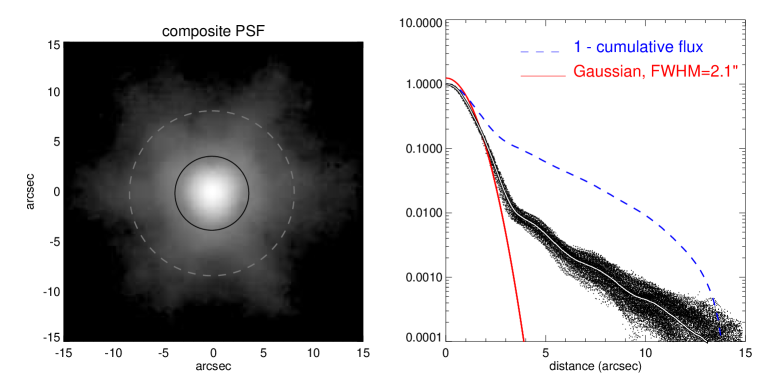
Figure 11: The composite PSF used in decompositions (shown in the left frame in log-scale to emphasize the wings: in the right frame the PSF is normalized to its maximum value). The red solid curve in the right indicates a Gaussian with the same FWHM=2.1″, approximately matching the inner part of the actual PSF (black symbols). The white curve on top of black symbols indicates an azimuthally symmetrized version of the composite PSF. The dashed blue curve indicates the cumulative flux outside a given distance from the center: the solid and dashed circles in the left, with radii $3.7\arcsec$ and $8.3\arcsec$ indicate the regions where 90% and 98% of the flux is concentrated (50% of flux falls within 1.3″). The composite PSF, oversampled with a factor of 5 (pix-size 0.15 arcsec, total size $30\arcsec\times 30\arcsec$) was provided by Tom Jarrett.

2.3 Generation of input files for GALFIT decompositions

The (ascii) input file for GALFIT specifies the galaxy data, mask, sigma, and PSF fits-files, and the region of the data image used in the decomposition. It also lists the components/functions used in the decomposition model, the initial guesses for the parameters, and specifies which of the parameters will be kept fixed, and which are iteratively varied in order to minimize the ${\chi^{2}}_{\nu}$. After convergence to a final solution, the final parameter values are written into an output file, with similar format as the input file. If needed, this output file can thus be used as an input for a new iteration (see Peng et al. 2002, 2010 for details).

The input file also specifies how to convert the image values to magnitudes. The data images from P1 are in flux units (MJy/sr). A conversion from pixel values $F_{i}$ to (AB) surface brightness and integrated magnitudes is done with the formulas:

$$\mu_{3.6} = -2.5\log_{10}F_{i}+5\log_{10}{pix}+zp$$ (13)

$$mag_{3.6} = -2.5\log_{10}\sum_{i}F_{i}+zp,$$ (14)

where $pix=0.75\arcsec$ and the zeropoint at 3.6 $\mu$m is $zp=21.097$ (P3, Muñoz–Mateos et al. 2014). Values of $pix$ and $zp$ are inserted into GALFIT input file.

All P4 input files for 1-component (Sérsic) and 2-component bulge+disk (Sérsic+exponential) decompositions were generated automatically. Similarly, template files were created for the multi-component decompositions, which contained, in addition to bulge and disk components, entries for a Ferrers-bar, and a central unresolved PSF-component. The user then manually choose which components are fit and which functions used in the final model (see Sect 3 for more details). In all our decompositions we keep the centers of the components fixed to the galaxy center. The cases were this is clearly not appropriate (galaxies with off-center bulges and bars) are noted in the parameter files.

1. In 1-component input files initial guesses are needed for five free parameters: the Sérsic index $n$, the effective radius $R_{e}$, the total magnitude $m$, the isophotal minor-to-major axial ratio $q$, and the position angle $PA$. The starting values of $m$ and $R_{e}$ were taken directly from the data (total galaxy magnitude and half-light radius), for the Sérsic index $n=2$ is inserted as an initial guess, and $q$ and $PA$ were set to arbitrary values (0.9 and $10^{\circ}$, respectively). We thus avoided using the measured outer isophotes, to force GALFIT to search through a wider parameter space while minimizing the ${\chi^{2}}_{\nu}$. Typically 1-component fits converged after 10-20 iterations. When the fit did not converge, or if the final parameters were nonphysical (say, $n>10$, $q<0.05$, very large or small $R_{e}$), a new decomposition was started manually with new initial guesses. Usually this did not lead to any improvement, indicating that GALFIT is indeed very efficient in avoiding spurious local minima.

2. The 2-component bulge-disk models apply a Sérsic-function for the bulge: they thus need guesses for the same Sérsic parameters as before, except that now these refer to the central component. Accordingly, we used the initial guess $R_{e}$ (bulge) = 0.5 $\times R_{e}$ (image) and $m_{bulge}=m_{image}+1$. For the disk we use either ’expdisk’ or ’edgedisk’-function, depending on the estimated galaxy inclination. In case of low or moderate inclination $b/a\gtrsim 0.2$ (corresponding to $i\lesssim 80^{\circ}$), we use the ’expdisk’ function, which needs two free parameters, the scale length ($h_{r}$) and the integrated magnitude of the disk, $m_{disk}$. We chose $h_{r}=$ 0.25 $\times R_{gal}$ and $m_{disk}=m_{image}+1$, thus starting with a model with fairly massive and extended bulge. The disk orientation was fixed to the shape of the outer isophotes determined from the image (see Sect 2.2.3). In case of a nearly edge-on disk, $b/a\lesssim 0.2$, we use the ’edgedisk’ function with four free parameters: the central surface brightness $\mu_{0}$, radial scalelength $h_{r}$, vertical scalelength $h_{z}$, and the position angle of the disk. The first guesses are $\mu_{0}(disk)=\mu_{0}(image)+3$, $h_{r}$ as for the expdisk-model, while $h_{z}/h_{r}=0.1$. The position angle is left free, with $PA_{outer}$ as an initial guess.

3. In the template files for the multi-component fits the initial bulge and disk parameters are set as for the 2-component models. For the Ferrers-bar the free parameters are the surface brightness at the effective radius of the bar, $\mu_{e}$, its outer truncation radius $R_{bar}$ (denoted with $r_{out}$ in Eq. (7)), its axial ratio, and its position angle. As initial guesses we choose $\mu_{e}$ (bar)=$\mu_{e}$ (image)+3, $R_{bar}=0.25\times R_{gal}$, $q_{bar}=0.5$, and $PA_{bar}=PA_{disk}+90^{\circ}$. For the magnitude of the unresolved central component we used $m_{psf}=m_{image}+5$. However, in practice we typically modified these pre-inserted template values even before starting the search of the final model, for example by adopting the output parameters from 2-component decompositions for the disk and bulge.

2.4 Visualization of GALFIT decompositions: GALFIDL Package

In its standard use, GALFIT is executed from the operating system command line, with an input file argument. This input file lists the input data files and the initial guesses for the parameters, as described above. The final decomposition parameters are written to an output file with a fixed name galfit.NN, where NN is a running number. Optionally, GALFIT makes a fits file containing the clipped data image (OBS; includes the region chosen for the fit), and total PSF-convolved model (MODEL), and the OBS-MODEL residual. Another GALFIT option is to write a FITS file containing model components in separate fits extensions.

In P4 we have used GALFIT via GALFIDL, which is a set of IDL routines designed for easy visualization of the output from GALFIT decompositions. In addition, GALFIDL includes wrapper routines for calling GALFIT from inside IDL, with the advantage that the GALFIT output files and the produced plots are automatically renamed in a systematic fashion, using the names of the input files. We have utilized this by coding the galaxy identification and decomposition model components to the name of each produced output file (see Appendix A)

The visualization options in GALFIDL follow those of the BDbar-decomposition program we developed earlier for the NIRS0S survey (Laurikainen et al. 2005), the most central of which is displaying a 2D plot of surface brightness vs. distance from the galaxy center (see Fig. 12). The advantage of this, compared to the more commonly used azimuthally averaged profile, is that the contributions of different model components, with different apparent ellipticities, are easily highlighted (Laurikainen et al. 2005; see also Gadotti 2008). The other visualization options include OBS-MODEL residual plots, profile cuts along a constant PA, comparison to observed profiles along isophotal major axis produced by IRAF ellipse, and plots showing schematically the different components included in the decomposition. The next section illustrates our decomposition strategies in more detail, concentrating on 2D-profiles. Additional plot types are illustrated in Appendix B, which describes the output released through a P4 web page for all S⁴G galaxies.

Figure 12: Schematic example of the 2D-profile plots. The black dots in the upper left frame show a synthetic observational image (exponential disk with added Poisson noise): the surface brightness (in arbitrary units) is plotted as a function of distance along the sky plane. The green dots indicate the best fitting GALFIT expdisk model; the width of the wedge-shaped profile depends on the disk inclination (here $i=60^{\circ}$). Note that this plot might leave an impression that the outer disk is not properly fitted: this illusion is due to the noise distribution appearing skewed in magnitude plots. The middle left frame illustrates the same model, after realistic noise (measured from the synthetic image) has been added also to the model profile, giving a visual confirmation that the model indeed is successful. The images in the right indicate the fitted model without (upper frame) and with noise (middle). The lowermost frames display a fit to a synthetic galaxy (image in the right) composed of a Sersic-bulge (here $n=2$, with circular isophotes), an exponential disk, and a Ferrers bar.

3 Building the final multi-component decompositions - examples

The final decompositions for S⁴G galaxies were done by fitting a maximum of 4 components. Typically the components were the bulge (B), disk (denoted either as D or Z, depending on whether the galaxy was close to edge-on), bar (bar) and the nucleus (N), but could be any combination of these. The ingredients of the model are indicated by concatenating the designations of the components to the final model name: this same naming convention is used in the names of decomposition output files stored to IRSA (Appendix A). Note that the component designation is based on the intepretation of the component, not the function used in the fit. A disk (’D’), though most often fit with the expdisk function (1969 cases), may also be fitted with ferrer2 (69 cases) or sersic functions (99 cases). Similarly, in six cases a bulge (’B’) was fitted with an expdisk or edgedisk, and in one case a ’bar’ with a sersic function. All elliptical galaxies were fitted with a single Sérsic and are designated as B).

In all final decompositions the orientation parameters of the outer disk were fixed and we also fixed $\alpha$ and $\beta$ in the Ferrers function ($\alpha$=2, $\beta$=0). All other parameters were left free for fitting. However, to find the structure components properly it was convenient to temporarily fix many of the model parameters at the beginning, and then release them one by one. For some galaxies, the length of the bar was kept fixed even in the final model. This was the case if GALFIT persistently gave a clearly incorrect bar length when compared to visual evaluation (in such a case the ${\chi^{2}}_{\nu}$ minimization was attempting to fit some other feature than a bar).

Altogether over 20 different combinations of components were used in the final decomposition models; Table 2 collects an inventory of the main categories. This diversity of models is motivated by our desire to measure the bulge (if present) and the underlying disk parameters in a reliable manner. Note that our definition of ’bulge’ is quite broad, based on the excess flux in the central parts of the galaxy over that associated with the disk and bar components (’photometric bulge’). The decompositions themselves do thus not attempt to judge the physical character of this component, whether a merger-related, velocity-dispersion supported classical bulge, or a rotationally-supported ’pseudo-bulge’ (Kormendy 1982), representing either a secularly formed central stellar disk component (Kormendy 1993) or a bar-related inner boxy/peanut component formed via bar vertical buckling (Combes & Sanders 1981; Athanassoula 2005). However, in Paper 2 we address the deduced bulge parameters ($n$, $B/T$) in the context of often-used classical/pseudo bulge indicators (Kormendy & Kennicutt 2004) and also make comparisons to compilations of pseudo-bulges identified based on their HST morphology and star formation properties (Fisher & Drory 2010).

In (non edge-on) galaxies with two distinct disk components (desgnated with dd, the inner disk was fit either with an exponential or a Sérsic function, depending on the flattening of the profile. Such inner disk components differ from our photometric ’bulges’ by their much shallower profiles; they are also usually associated with a distinct inner spiral structure. Small central components were fit with the PSF, indicated as ’N’ in the model names. However, because of the limited resolution of S⁴G images, many of those structures, particularly in late-type spirals, might actually be small bulges rather than nuclear point sources. Typically these components contribute less than a few percent of the total flux.

Table 2: Main categories of final decomposition models.

Disk: moderate inclination			1889
	BD	311
	BDbar	213
	ND	214
	NDbar	184
	Dbar	458
	DD	125
	D	367
Disk: nearly edge-on			362
	BZ	55
	NZ	62
	Zbar	8
	ZZ	113
	Z	126
elliptical:	B		26
ALL			2277

Note. — Final decompositions were made for 2277 galaxies: in case of low or moderate inclination (apparent $\epsilon\lesssim 0.8$), the disk component was fitted with expdisk-function, while for nearly edge-on galaxies ( $\epsilon\gtrsim 0.8$), the edgedisk-function was used. In models BD and BZ, a bulge component was identified besides a disk, and it was modeled with a Sérsic-function. These models may also contain additional disk components or unresolved central components (modeled with psf). The models BDbar include those bulge+disk systems which contained also a bar (modeled with ferrer2). In ND or NZ models the central component is modeled with PSF instead of Sérsic-function. This may represent either a true central point source or (more commonly) an unresolved bulge. The models NDbar include also a bar. The models Dbar and Zbar have no inner Sérsic or psf-components, but include a bar-component. They may also contain an outer disk component. The DD models contain both an inner and outer disk (and no bulge nor bar), while D models refer to pure disks. Similarly Z models apply a single edgedisk-function, while ZZ models contain both thin and thick disk-components.

3.1 Non-barred galaxies:

The decompositions were made starting from simple 1 and 2-component models, and then adding as many components as necessary. For non-barred galaxies the process leading to the final model was the following:

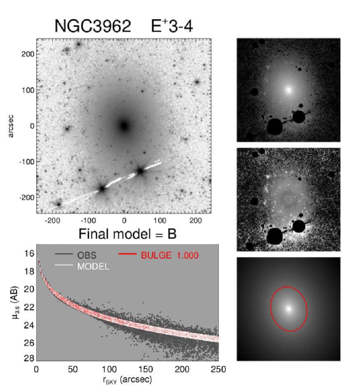
Figure 13: Figs. 13 -22 show the examples of final decompositions described in the text. In the big panel the galaxy image is shown in an inverted logarithmic scale (magnitude range $27>\mu_{3.6}(AB)>18$), clipped to display the main morphological characteristics. The three small panels show the masked original image (upper right panel), the model image (lower right), and the residual OBS-MODEL in the middle (range $\pm 1mag$; white indicates excess light over the model). The lower left frame shows the 2D profiles of the observed and model images (black and white dots), together with the model components (colors; labels indicate the relative fraction of flux in this component; in this particular case there is only one component). The same components are also marked, with the same colors, on the lower right model image: the semimajor axis of the ellipse corresponds to $2R_{e}$ of the component in question. The mid-IR classification from Buta et al. (2014) is also indicated. In this particular example for NGC 3962, the single Sérsic fit provides an acceptable final model. The overall profile is close to a de Vaucouleurs profile (Sérsic $n=5.6$) in accordance with the morphological classification (E). Nevertheless, the slight bends in the profile and the structure in the residual image suggests that if desired, it would have been possible to get an even slightly better fit by including multiple components.

(1) Accepting the automatic 1-component model (single Sérsic) as the final model. This was the case for elliptical galaxies (see NGC 3962 in Fig. 13).

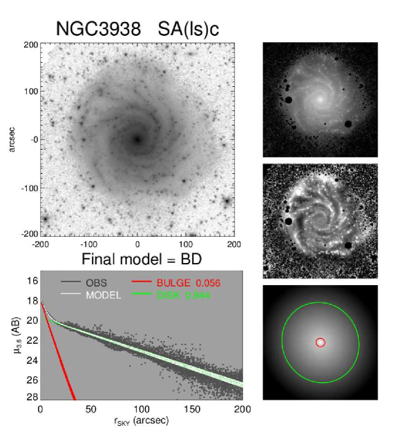
Figure 14: NGC 3938: Example of a galaxy in which the automatic Sérsic bulge + exponential disk fitting gave an acceptable final solution. In the profile plot the spirals appear as small undulations on the generally well-fitted disk. The labels in the profile plot indicate the relative fraction of flux in various components.

(2) Accepting the automatic 2-component bulge/disk decomposition as a final model. A typical example is NGC 3938 (Fig. 14).

(3) Adopting a bulge/disk model, after interactively finding modified initial parameters that converged to an acceptable final fit.

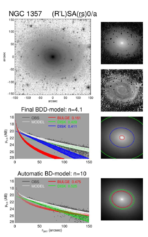
Figure 15: NGC 1357: The surface brightness profile of this galaxy shows a small bulge and a large, fairly exponential disk. However, the automatic bulge-disk fit would give an unreliably large bulge extending through the whole galaxy (lowermost row). A more reasonable fit is obtained by adding another exponential disk component to the inner part of the galaxy (upper profile). This inner component corresponds to the region of tightly wound spiral arms with higher surface brightness.

(4) Adding a nucleus component or an inner disk (e.g. NGC 1357, Fig. 15) to the bulge/disk model.

(5) When the galaxy had no obvious bulge we started from a single exponential disk, and if necessary, a second disk and/or nucleus was added (see NGC 723, Fig. 16).

When the outer profile was affected by a possible stellar halo, the outermost part of the profile was not fitted. The best model was vetted by looking at the original image, the residual image after subtracting the model, the 2D surface brightness profile, and the ellipticities of the structures. The value of final ${\chi^{2}}_{\nu}$ was not used as a criterion in assessing the relative merits of the models (often a simpler final model was preferred even if a more complicated model would have yielded slightly smaller reduced ${\chi^{2}}_{\nu}$).

Also, it is well known that many elliptical galaxies have small inner disks (Rest et al. 2001), and it has been shown by Huang et al. (2013) that many elliptical galaxies are better fitted with multiple Sérsic profiles. Nevertheless, such a detailed approach was not taken in this study, in which the emphasis is in the analysis of disk galaxies (paper 2). It is worth noticing that while using deep images like those in $S^{4}G$, in an automatic fit the bulge profile even in late-type spirals is easily degenerate with the outer part of the disk. In automatic fits this may lead to an unrealistically large Sérsic $n$ and $R_{e}$ for the bulge, of which NGC 1357 is a good example (Fig. 15).

3.2 Barred galaxies:

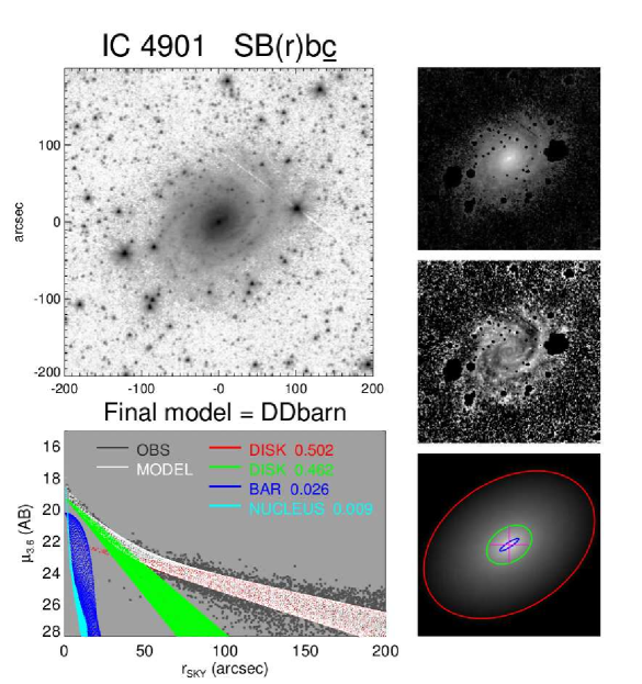
Figure 19: IC 4901: An example of a barred galaxy, in which the disk is fitted with two exponential functions. Additionally, a small central psf-component is included, marked as a cross on the model image. The inner disk corresponds to the higher surface brightness part of the disk outside the bar, where the spiral arms are also prominent.

For barred galaxies a similar step-wise approach was followed. NGC 936 (Fig. 17) and NGC 5101 (Fig. 18) are good examples demonstrating the importance of preventing the bar from mixing with the bulge flux. Adding a bar component to a simple bulge/disk model drastically changes the obtained properties of the bulge (for NGC 936 $B/T$ drops from 0.46 to 0.19; for NGC 5101 from 0.99 to 0.22). NGC 5101 has also a type II profile in the disk break/truncation classification associated to a broad outer ring (Laine et al. 2014). Using the edge of the ring as a manifestation of a different flux distribution in the outer disk might be a bit misleading. Because of such ambiguities in the interpretation, we typically fit the type II disk profiles with a single exponential component. However, there are other barred galaxies in our sample, such as IC 4901 (Fig. 19), in which two exponential components (+ Ferrers function for the bar) were used for fitting the disk. In this particular galaxy using two exponentials is necessary, and those clearly correspond to distinct surface brightness components. Note that the outer disk of NGC 5101 is clearly lopsided (see the residual plot in Fig. 18). Such asymmetries are not taken into account in the pipeline decompositions (in case of strongly distorted galaxy no final model was made). See Zaritsky et al. (2013) for a detailed study of galaxy lopsidedness using S⁴G images.

3.3 Pure disk galaxies:

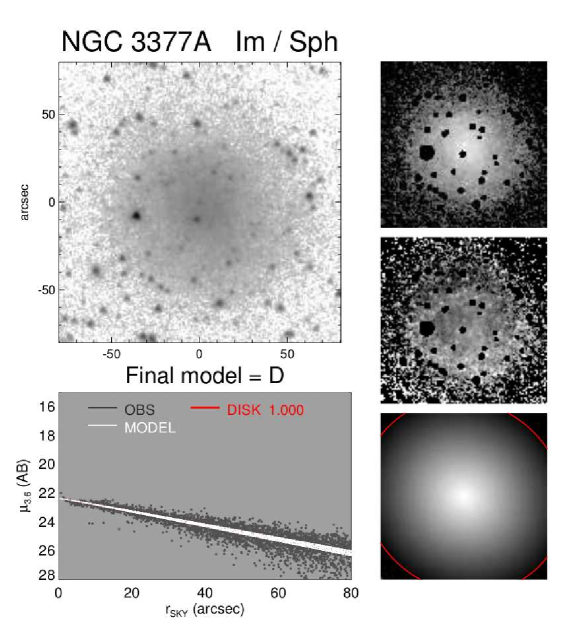
Figure 20: NGC 3377A: A bulgeless disk galaxy, well fit with a single exponential function.

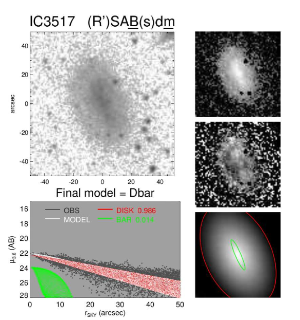
Figure 21: IC3517: Another example of a bulgeless disk galaxy. The surface brightness profile is well fit with a single exponential function. However, the image shows also an elongated inner structure, which can be fitted with a Ferrers function.

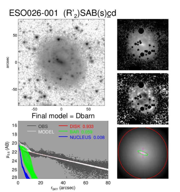
Figure 22: ESO026-001: An example of a galaxy in which the disk is fitted with an exponential function, although a Sérsic function with $n<$1 would have given a more precise fit to the disk.

A third main group of galaxies in our sample are those having no obvious bulge. They may have a single exponential disk (NGC 3377A in Fig. 20), or more than one disk components (NGC 723 in Fig. 16). The structure fit as an inner disk in NGC 723 consists of broad, prominent, and tightly wound spiral arms. Bulgeless galaxies may have bars, of which NGC 3517 (Fig. 21) is an example. To get an homogeneous estimate for the scale length of the disk for these galaxies, the outer disks were always fit with an exponential function, even in galaxies where the disk would have been somewhat better fit by a Sérsic function with $n$ slightly less than unity. Generally, the assumption of an exponential disk is good, but there are also cases, like ESO026-001 (Fig. 22) in which a Sérsic function would actually be a better choice.

3.4 Edge-on galaxies:

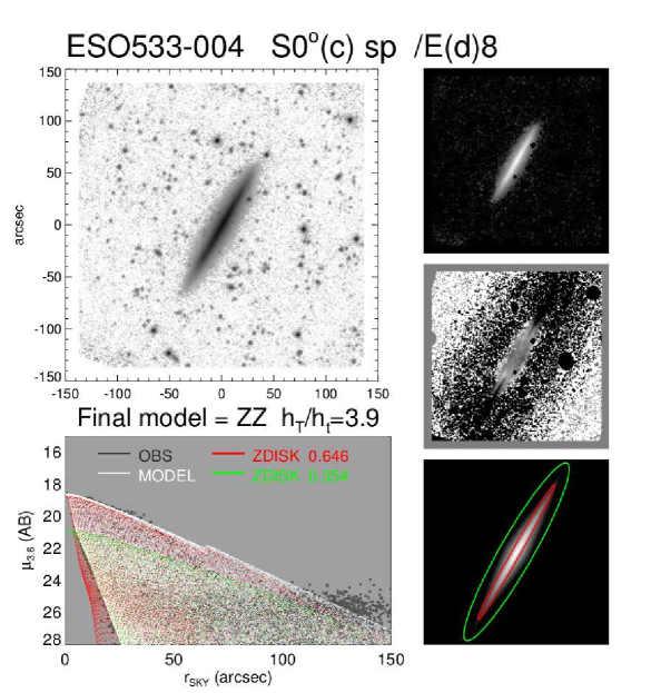
Figure 23: ESO533-004: An example of an edge-on galaxy fitted with two disk components: the ratio of thick disk to thin disk scale heights is $h_{T}/h_{t}=3.9$ and the thick disk contains 35% of the total model luminosity. For comparison, the detailed vertical profile fits in Comeron et al. 2012 indicated $h_{T}/h_{t}=4.3-4.6$ depending on the radial location, with about 45% of light in the thick dist component.

The GALFIT models for the nearly edge-on galaxies assume that the disk is viewed completely edge-on. A bulge, and in some cases also a bar or an additional thick disk component were included (Fig. 23). In these models also the vertical thickness was an output parameter. However, these models are tentative, and are meant solely as starting points for better, scientifically oriented decompositions. There already exists detailed modeling of edge-on galaxies in S⁴G, based on fitting their vertical profiles to hydrodynamical thin-thick disk models (Comerón et al. 2011, 2012). Their radial luminosity profiles have been analyzed in(Comerón et al. 2012, 2014; Martín-Navarro et al. 2012).

3.5 Scope of pipeline decompositions

The P4 models for the spiral galaxies $T>0$ are generally good, giving reliable estimates for parameters such as the bulge-to-total flux ratio ($B/T$), the scale length of the disk ($h_{r}$) and its central surface brightness ($\mu_{0}$). However, despite the fact that up to four components were fit, the pipeline decompositions for the early-type disk systems (T$\lesssim$1), because of their complex structures, are often insufficient. These systems may have nuclear bars, ovals and lenses, which are not included in our models in any systematic fashion. Because of this, the pipeline $B/T$ flux-ratios, particularly for S0 galaxies, can be over-estimated. Including all these structures will require even more complex decompositions, such as those done in the near-IR by (Laurikainen et al. 2005, 2006, 2009, 2010). Such time consuming modeling goes beyond the scope of our current P4 decompositions; nevertheless, the P4 decomposition output files provide good starting point for further fine-tuning.

Figure 16: NGC 723: This is a disk galaxy with no centrally concentrated bulge component, but it is clearly not a single exponential galaxy. The bump in the surface brightness profile corresponds to the strong high surface brightness spiral structure in the inner parts of the galaxy, here fit with a nearly flat part (Sérsic function with $n=0.12$).

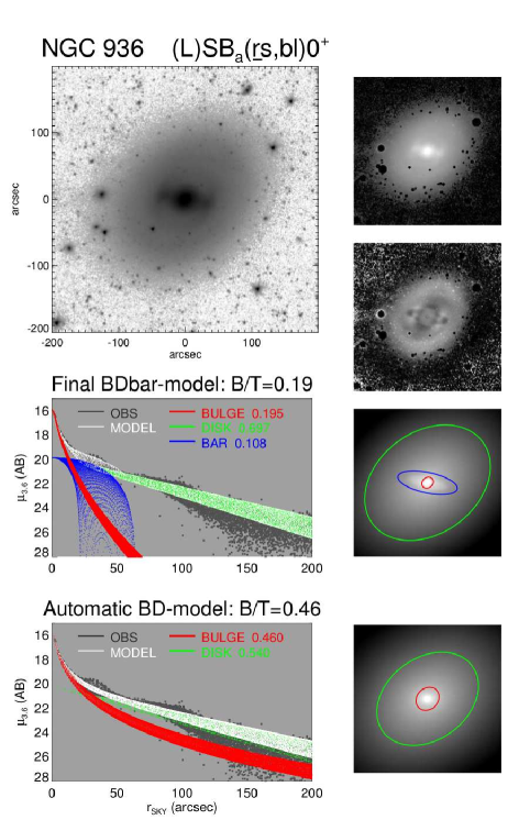
Figure 17: NGC 936: An example of a barred galaxy where inclusion of a bar component to the model makes a large difference in the bulge parameters. The lowermost row shows the automatic bulge/disk model, whereas the upper panels include a bar component. In the simple model, the bar flux is degenerate with the bulge flux. Multi-component decomposition is thus essential for getting a realistic bulge-to-total flux ratio: the B/T = 0.46 in the BD-model, but drops to 0.19 in the BDbar model .

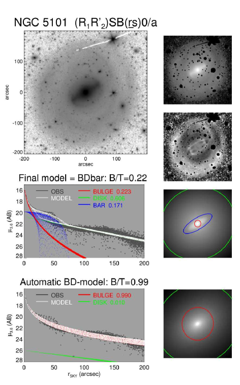
Figure 18: NGC 5101: Another example of BDbar decompositions where inclusion of the bar components is essential in getting realistic bulge parameters. Note also that in the final model the underlying disk is fit with an exponential function, although the outermost profile is downbending (Type II break/truncation). However, the steeper outer slope seems to be associated with a broad double outer ring, rather than a fundamentally distinct outer disk component.

4 Uncertainties of the decomposition parameters

The formal uncertainties of the decomposition parameters have little significance, as they refer to purely statistical uncertainty due to image noise based on the assumption that the model is accurately describing the true underlying light distribution. Taking into account the complex morphology of most galaxies, this assumption is clearly not valid (see Peng et al. 2010 for detailed discussion of errors). Related to this, the final value of the reduced ${\chi^{2}}_{\nu}$ is a poor indicator of the goodness of the fit (even for a good model it is typically much larger than unity) and is thus not used as a decisive factor in choosing the preferred final model. In practice, the choice of the final model components plays a crucial role: for example as seen in Section 3, omission of the bar component when a bar is present may lead to seriously biased bulge parameters. In this Section we perform a systematic comparison of bulge and disk parameters between 2-component and final multi-component models. We also first examine the potential uncertainties related to the preparation of data before the decompositions, namely the used PSF-function, the effect of sky subtraction uncertainty and the sigma-image.

4.1 PSF

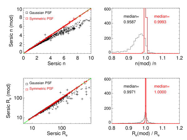
Figure 24: The effect of the PSF on decomposition parameters. The plots on the left show the Sérsic index and effective radius in 1-component fits using modified PSFs instead of the standard composite PSF: black symbols indicate results using a Gaussian PSF (wings truncated), and red points when using a symmetrized composite PSF. Larger black (red) symbols indicate points deviating by more than 25$\%$ (10$\%$) from the unit line. In the right panels the histograms of the relative changes in the parameters are shown: black and red colors have the same meaning as in the left frames.

As illustrated in Fig. 11, the IRAC PSF has extended wings. Moreover, the PSF and the orientation of its asymmetric extensions vary from image-to-image, which has not been taken into account in our decompositions. To check the importance of the PSF wings, we compared differences in decomposition parameters obtained when the adopted composite PSF was replaced with a Gaussian PSF having the same $FWHM=2.1\arcsec$. Fig. 24 compares the resulting effect on the Sérsic parameters in 1-component models. Clearly, decompositions with the Gaussian PSF yield $n$ values that are systematically too small, differences reaching even tens of percents for some of the galaxies (though the median deviation is less than 5$\%$). However, these rather large deviations are not representative of the true uncertainties, but rather give an idea of the magnitude of the error if the tails of the PSF were altogether ignored. A better measure of the actual uncertainty in P4 decompositions is obtained by comparing with an azimuthally symmetrized version of the composite PSF. Clearly, now the differences in $n$ are much smaller (see the red symbols in Fig. 24).

We also checked the influence that the PSF has on the multi-component models. For that purpose we rerun all final decompositions that included both bulge and disk components (+ possible bar and center components; total of 524 models after excluding nearly edge-on galaxies), using both the Gaussian PSF and the symmetrized PSF. Table 3 lists the median of relative differences in bulge $B/T,n$, $R_{e}$, disk scale lengths $h_{r}$, and bar-to-total ratio Bar/T, when compared to the results obtained using the standard composite PSF. The largest differences are seen for the Sérsic parameters while using the Gaussian PSF, whereas $h_{r}$ is barely affected. On the hand, the differences in parameters between those obtained using the composite PSF and using the symmetrized version are negligible. Based on these results we conclude that the spikes of the PSF have no significant effect as long as the nearly circular wings of the PSF are included. The use of single composite PSF for all S⁴G images should thus be acceptable.

4.2 Sky subtraction

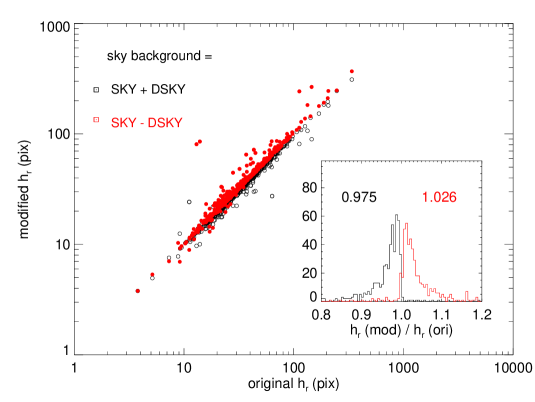
Figure 25: The effect of sky background subtraction on the disk scalelength. All final decomposition models including both a bulge and disk (and possibly additional bar and central components) were rerun using images where the assumed sky background was modified by $\pm DSKY$, where $DSKY$ is the conservative estimate of global sky variations in the image (see Section 2.2.3).

In principle, poor sky subtraction can severely affect the decomposition results, in particular the parameters of the disk. To constrain the possible magnitude of such uncertainties, we rerun the multi-component decompositions that included both bulge and disk components (+ possible bar and center components; same 524 models as above). Two additional sets of sky values, $SKY^{\prime}=SKY\pm DSKY$, were used, where DSKY was the standard deviation of the different sky regions. Fig. 25 shows the effect on the scalelength of the disk. Although individual changes can in few cases be large ($h_{r}($mod)$/h_{r}($ori$)>1.2$ in 9 cases when too small a sky is subtracted), the median differences are less than 2% (and even smaller in the other parameters of interest, see Table 4). The sky subtraction is not a concern in the current decompositions.

4.3 Sigma-image

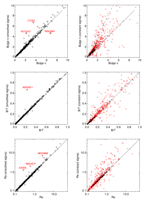
Figure 26: Sensitivity of estimated bulge parameters (Sersic $n$, bulge-to-total flux ratio $B/T$, effective radius $R_{e}$ in kpc’s) on the used $\sigma$-image. In the left column, we have smoothed the P4 $\sigma$-images with $5pix\times 5pix$ median filter, while in the right it has been replaced with a constant $\sigma$. The scatter plots show the modified parameter values versus the original ones. In the right, the red open and black filled circles refer to galaxies with mid-IR type $T\leq 4$ and $T\geq 5$, respectively. Lines corresponding to one-to-one correspondence are drawn in each frame: in the right uppermost frame the dashed line indicates $n_{mod}/n_{ori}=2$.

The weights applied to various pixels have an important role in decompositions, in particular when the galaxy structure is complicated, so that the differences between the applied model and the true structure are large. As mentioned in Section 2.2.5 the $\sigma$-image itself is a statistical estimate of the underlying $\sigma$ in each pixel, so it might be reasonable to smooth it before applying it in the decompositions. In Fig. 26 (left column) we examine the effect of sigma-image smoothing on the derived bulge parameters. A median filter is applied with a width of 5 pixels. Clearly the effect is quite small except for a few deviant cases marked on the plot. In these cases the bulge parameters are sensitive also to changes in the PSF or the sky background level.

For comparison, Fig 26 (right column) also illustrates the changes in bulge parameters if a constant sigma is assumed at all image pixels. A constant sigma exaggerates the relative weight of the central regions compared to the outskirts. Besides a large scatter, also a systematic increase of the estimated $n$ is obvious: the median $n_{mod}/n_{ori}=1.2$ (the mean ratio is 1.4). What typically happens is that the fit tries to reproduce the central peak with an increased $n$, even if the outer disk then becomes too much bulge dominated. Indeed, the bias (and the scatter) is particularly large for earlier type disks (open circles in the plot indicate $T\leq 5$; median $n_{mod}/n_{ori}=1.25$). This comparison reminds us that when decomposition parameters from different studies are compared, it is also important to pay attention that similar weights have been applied.

4.4 Two-component versus multi-component decompositions?

Automatic 2-component Sérsic-exponential (or Sérsic-Sérsic) models are often applied to large data surveys. This is a natural approach as the data quality (depth/angular resolution) might be insufficient for more detailed modeling so that the large effort in multi-component decompositions does not seem justified. Moreover, it has been recently claimed (Tasca & White 2011) that 2-component decompositions (Sérsic + exponential) are sufficient also for fitting barred galaxies. Their argument was based on obtaining similar average $B/T$ ratios for barred and non-barred galaxies in their 2-component bulge/disk models. They reasoned that if the omission of the bar were a problem it should manifest as a higher B/T for barred galaxies. However, to accurately address this matter one has to compare the different types of decompositions (2-component and multi-component) for well-defined samples of barred/non-barred galaxies.

Such a comparison between different decomposition models is shown in Fig. 27. Again, those galaxies for which the final model contains both a bulge and a disk are studied. For the non-barred galaxies (those with no bar-component; leftmost column in the Figure) the bulge parameters (Sérsic $n$, $B/T$, $R_{e}/h_{r}$) in automatic 2-component runs are almost identical to those in the final models. This agreement is expected because over 80% of the final non-bar models are just Sérsic-expdisk models (15% have two disk components, and 2% have an extra central component), and typically the automatically found BD models did not need any refinement. For barred galaxies (those with a bar-component in the final model; middle column), the obtained median values depend drastically on whether the bar is included. This result emphasizes that the examples of decompositions given in Section 3, highlighting the importance of modeling the bar (e.g. Figs. 17 and 18) were not exceptional cases. Overall, ignoring the bar increases the estimated $B/T$ ratios by a factor of 2-3 because of gross (even by as much as a factor of 5) overestimate of $R_{e}$ and $n$. For example, for spirals in the range $1\leq T\leq 5$ the 2-component decompositions suggest $n\gtrsim 4$ whereas the multi-component runs indicate $n\approx 1-2$. Altogether, in the final models the difference in bulge parameters obtained in the multi-component decompositions for barred and non-barred galaxies is fairly small (right column in Fig. 27).

The conclusion that multi-component decomposition models are essential to measure realistic bulge parameters for barred galaxies is not new (Laurikainen et al. 2006, 2007; Gadotti 2008; Weinzirl et al. 2009)). A similar conclusion, based on synthetic images, was reached also by Laurikainen et al. (2005).

In Fig. 28 we compare the combined bar/non-barred sample of the previous figure with the decompositions in Laurikainen et al. (2007). Because of the large fraction of barred galaxies, the difference in the obtained bulge properties between the 2-component and multi-component decompositions remains significant, even when barred and non-barred galaxies are considered together. We find an excellent agreement between the current multi-component results and those in Laurikainen et al. (2007), obtained with a different decomposition code (BDBAR; however BDBAR uses IDL Curvefit and is thus based on the same Levenberg-Marquadrdt minimization as GALFIT), and based on different near-IR image data. It is worth noticing that in these decompositions the Sérsic $n$ for Hubble types Sa-Sc is nearly $n\sim$1, whereas in the decompositions by Tasca & White (2011), for the same Hubble types, the Sérsic index is peaked at $n\sim$4. Small values of the Sérsic index, similar to ours for these Hubble types, are reported also by Graham & Worley (2008).

Table 3: The effect of a modified PSF on final decomposition model parameters

		GAUSSIAN  PSF			SYMMETRIZED  PSF
		median($D$)	median($|D|$)		median($D$)	median($|D|$)
$B/T$		-1.5 %	4.5 %		-0.1 %	0.2 %
$n$		-3.0 %	7.8 %		0.0 %	0.5 %
$R_{e}$		8.9 %	9.8 %		0.1 %	0.3 %
$h_{r}$		0.0 %	0.3 %		0.0 %	0.0 %
$Bar/T$		-1.5 %	4.4 %		-0.1 %	0.2 %

Note. — $D$ stands for the relative difference (e.g. $D=[n($mod$)-n($ori$)]/n($ori$)$), where ’ori’ refers to the standard composite PSF. Medians are used to characterize the typical deviations and the scatter, to eliminate spurious cases where the decompositions with Gaussian PSF converged to a different type of solution.

Table 4: The effect of sky subtraction on final decomposition model parameters parameters

		SKY + DSKY			SKY - DSKY
		median($D$)	median($|D|$)		median($D$)	median($|D|$)
$B/T$		0.2 %	1.5 %		-0.1 %	1.6 %
$n$		-1.4 %	1.8 %		1.8 %	2.0 %
$R_{e}$		-1.2 %	1.4 %		1.7 %	1.8 %
$h_{r}$		-2.5 %	2.6 %		2.6 %	2.8 %
$Bar/T$		0.2 %	1.5 %		-0.1 %	1.6 %

Note. — $D$ stands for the relative difference (e.g. $D=(n(mod)-n(ori))/n(ori)$), where ’ori’ refers to the standard sky subtraction.

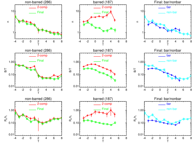
Figure 27: Comparison of bulge parameters between automatic 2-component and final multi-component decompositions. The morphological type $T$ is from the Buta et al. (2014) mid-IR classification. Comparison is made for the galaxies for which the final model included both bulge and disk components. In the left frames decompositions for non-barred galaxies are compared, while the middle frames show those with a bar component in decompositions. In the right frames the final decompositions for barred and non-barred galaxies are compared. The symbols stand for median values in bins with five or more galaxies, error bars are errors of the mean values in the bin. Note that the Buta et al. (2014) classification contains also half-integer values of $T$, resulting from averaging over two rounds of classification. However, the number of galaxies with half-integer values is much less than those with integer $T$. Therefore, when binning the galaxies we have rounded the half-integer values randomly to the nearest smaller or larger integer value; same is done in Fig. 33 below.

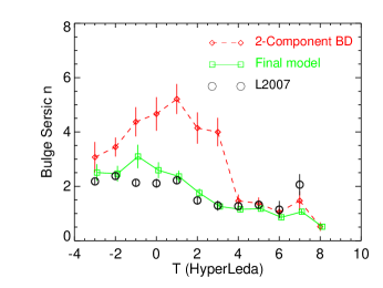
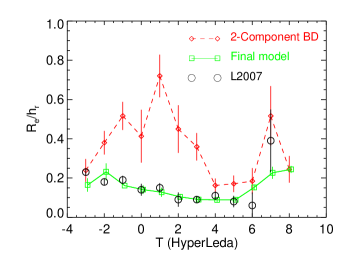
Figure 28: Comparison of final S⁴G decompositions parameters to those of Laurikainen et al. (2007; the values are tabulated in Table 2 in Laurikainen et al. 2010) multi-component decompositions for NIRS0S ($K_{s}$ band, 143 galaxies with $-3\leq T\leq 1$ ) and OSUBSGS (H band, 129 galaxies $2\leq T\leq 7$) data. The S⁴G results show 524 galaxies for which the final decomposition model contained both a disk and a bulge component (excluding nearly edge-one galaxies). For comparison, also the results of semi-automatic 2-component decompositions are shown. The symbols stand for the median values in each bin with 5 or more galaxies, while the error bars denote the error of the mean. Note that here we use the optical classifications from HyperLeda, to facilitate comparison with previously published results.

4.5 Disk breaks

One of the main goals of Pipeline 4 is to obtain measurements for the galaxy size-magnitude scaling relations. In order to be consistent with earlier analysis (e.g. Courteau et al. (2007)) the P4 final models as a default use single exponentials for the disk. However, deep optical and near-IR surveys (Erwin, Beckman & Pohlen 2005; Pohlen & Trujillo 2006; Gutiérrez et al. 2011; Muñoz-Mateos et al. 2013) have shown that only a fraction of galactic disks ($\sim 1/3$) are simple exponentials (=Type I in Pohlen & Trujillo 2006 classification). Instead the typical brightness profiles consist of two (sometimes three) exponential subsections with different radial slopes. When the outer disk has a steeper slope, the galaxy is classified as possessing a Type II break (’truncation’), and conversely if the outer slope is more shallow, it is classified as a Type III break (’antitruncation’). Kim et al. (2014) have recently made 2D decompositions for 144 barred S⁴G galaxies taking into account disk breaks in their decompositions with the BUDDA code (de Souza et al. 2004; Gadotti 2008, 2009). Their fitting function for the disk consists of two exponential sections, with different scale-lengths ($h_{in}$ and $h_{out}$) inside and outside the break radius $R_{break}$. They also made decompositions where they fitted the disk with a single exponential component. Their result indicate that the inner scale lengths for two-component disks are typically about 40% longer than the scalelengths obtained in single disk fits; they thus conclude that “it is important to model breaks in Type II galaxies to derive proper disk scale lengths.”

Nevertheless, it is not always obvious what is the ”proper” disk scale length estimate to use in various scaling relations, in case the galaxy exhibits several exponential subsections. For example, it is well known (Pohlen & Trujillo 2006) that Type II breaks are often connected to outer rings associated with bar OLR resonances. Such breaks are indeed dominant for early type barred disks ($T<3$; Laine et al. 2014). Since the bar torques are able to push material from the CR regions out toward OLR, this will promote a shallower distribution inside the break radius. However, beyond the OLR the effect of bar is insignificant, so that the underlying disk can remain more or less intact. In such a case it might in fact be the outer, rather than the inner scalelength that would better characterize the original overall mass distribution. On the other hand, for later Hubble types the Type II break is often connected with the end of prominent spirals (Laine et al. 2014) and could be due to suppressed star formation: for such a case the inner scale length might indeed be more appropriate to characterize the disk as a whole. Laine et al. (2014) also find that for such spiral-related breaks the ratio $h_{inner}/h_{outer}$ is typically closer to unity than for OLR related breaks.

Figure 29 compares Pipeline 4 decompositions with several recent disk truncation studies, which use subsamples of the same S⁴G dataset. In this plot the disk scalelengths are displayed against the stellar mass derived in P3 (Muñoz–Mateos et al. 2014). Besides the above-mentioned Kim et al. (2014) 2D decomposition study, we also compare with Muñoz-Mateos et al. (2013) and Laine et al. (2014), where fits to 1-dimensional profiles were conducted. First of all, the Figure (upper row) indicates a very good agreement for the scale lengths of Type I profiles between all four studies, conducted with independent methods. Secondly, it illustrates the significant difference between the inner and outer slopes for Type II (and III) profiles, amounting to roughly a factor of two (see Muñoz-Mateos et al. 2013, Kim et al. 2014) . The P4 single disk scalelengths seem to fall quite close to being a geometric mean of $h_{inner}$ and $h_{outer}$ derived in earlier studies.

To emphasize the possible ’unperturbed’ nature of Type II outer disks, we compare in Fig. 30 the P4 scale lengths vs. stellar mass for Type I galaxies with the type II outer scale lengths derived in the above mentioned disk break studies. Indeed the differences between the Type I single disk $h$ and the Type II $h_{outer}$ are quite small, much smaller than the differences compared to $h_{inner}$. The fits to the data also give the impression that $h_{inner}/h_{outer}$ ratio gets closer to unity for less massive galaxies: this is in accordance with the above mentioned dominance of spiral-related less abrupt truncations for later and thus on average less massive spirals.

The Pipeline 4 single exponential fits have a convenient feature of representing an effective average over inner and outer disks (when both present). They thus provide a homogeneous set of robust scale measurements, not sensitive to factors modifying the local slopes. Nevertheless, a possible caveat is that the fitted effective single $h$ might become dominated by different degrees by the inner/outer parts, depending on the galaxy surface brightness. For example, the estimated $h$ might be biased toward $h_{inner}$ when the disk central surface brightness decreases toward less massive galaxies: this would be the case if the image depth was not sufficient to cover the galaxy regions beyond the break radius. Fig. 31 addresses this potential problem by comparing the trends of the break radii with respect to galaxy mass, to that of the galaxies’ visual outer extent ($R_{gal}$, see Sect 2.2.3; a similar trend would result if $R_{25.5}$ were plotted instead of $R_{gal}$). The figure indicates that a break, if present, should be detectable through the whole range of S⁴G galaxy masses.

In summary, we feel confident that the single disk fits provide a useful overall estimate of the disk original scale length (and its extrapolated surface brightness), though especially in case of barred massive galaxies secular evolution might have led to significant deviations from simple exponentials, important to include in detailed models for individual galaxies. Moreover it is likely that the slope differences associated with breaks are smaller for later types, which form a vast majority of S⁴G galaxies.

Nevertheless, as concluded by Kim et al. (2014), estimates of other decomposition parameters, such as the B/T ratio for massive galaxies would become more accurate if the inner slopes are accounted for (say, leading to less disk light assigned to bulge). The situation is somewhat analogous to the benefit of including additional inner components like bars (Laurikainen et al. 2005; Gadotti 2008), lenses in S0s (Laurikainen et al. 2010), or barlenses (Laurikainen et al. 2014) into decompositions. However, for the goals of Pipeline decompositions, the expected magnitude of changes (about 10% relative change in B/T according to Kim et al.) is quite small, compared to the uncertainties related to choice of the decomposition model components (say, including a bar versus ignoring it). The choice of the code might also sometimes have a bigger effect. For example, Kim et al. (2014) use NGC 936 as an example of Type II galaxy (see their Fig. 4). For this galaxy they fit a break at $98\arcsec$ and derive $h_{inner}=53\arcsec$ and $h_{outer}=28\arcsec$, all very close to the measurements in both Muñoz–Mateos et al. (2014) and Laine et al. (2014). On the other hand, the Pipeline 4 single disk fit (see Fig. 17) gives $h=40\arcsec$. We verified that truncating the disk in GALFIT decompositions at the break radius given in Kim et al., reproduces their inner slope quite well (we get $57\arcsec$). At the same time, the $B/T$ we obtain increases slightly (from 0.19 to 0.22), as anticipated by Kim et al.. Nevertheless, the $B/T$ we obtain after accounting for the more shallow inner slope is still nearly $50\%$ smaller than the value obtained by Kim et al. ($B/T$=0.32), probably because of some model/code dependent factors, such as how the image pixels are weighted, or the PSF is treated.

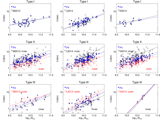
Figure 29: Comparison of P4 single disk scalelengths with decomposition studies including disk truncations. In the left frames the $h_{r}$ vs. stellar mass, obtained in P4 (blue symbols) are compared with the results in Muñoz-Mateos et al. 2013 (M2013) and Laine et al. 2014 (L2014), where the inner and outer scalelengths ($h_{inner}$ and $h_{outer}$, denoted with black and red symbols, respectively) were estimated for S⁴G galaxies from fits to 1-dimensional profiles. On the right, similar comparison to Kim et al. 2014 (K2014), who used 2D BUDDA decompositions for 144 barred S⁴G galaxies. In the uppermost frames Type I disks (no breaks) are compared: the lines show orthonormal fits to the measurements (orthogonal deviations minimized using the IDL PCOMP routine). In the middle same for Type II profiles: the dashed blue line indicates a fit to geometric means of the inner and outer scalelengths. In the lowermost frame: galaxies with Type III breaks.

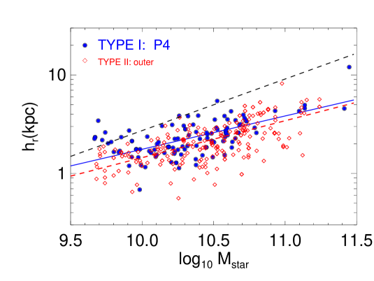
Figure 30: Comparison of P4 scalelengths for Type I galaxies (blue points), with the outer scalelengths of Type II profiles (red points; these combining Muñoz-Mateos et al. 2013, Laine et al. (2014) and Kim et al. (2014) measurements). Also shown are the corresponding orthonormal fits (solid blue and dashed red lines, respectively). The black dashed line shows a fit to inner scalelengths derived in the above mentioned studies (individual measurement points not shown). Note that the trend of single scalelengths in Type I galaxies resemble much more the outer scalelengths in Type II’s rather than the inner scalelengths.

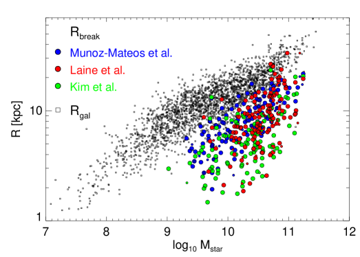
Figure 31: Comparison of the break radii between the inner and outer disk segments in the studies of Muñoz-Mateos et al. (2013), Laine et al. (2014) and Kim et al. (2014); large and small circles refer to Type II and Type III breaks, respectively. Note that the break radius drops rapidly with galaxy stellar mass. Also shown by small squares is $R_{gal}$, the P4 visual estimate of the galaxy extent in S⁴G images. The plot suggest that even in the case of low-mass, low surface brightness galaxies the depth of the S⁴G images is sufficient to assure that the break, if present, is not likely to be buried in the sky background.

5 Decomposition parameters

In the current paper (paper 1) we provide all the 1-component and final multi-component decomposition parameters in a tabular format (Tables 6 and 7), together with quality assignment flags. A brief check of how the major categories of the final models distribute among different Hubble types is also shown. All actual analysis will be presented in paper 2.

5.1 Quality assessment

The full S⁴G sample contains 2352 galaxies, chosen according to their internal extinction corrected B-magnitude ($M_{Bcorr}<15.5$), apparent B-band 25-mag isophotal diameter ($D_{25}>60\arcsec$), galactic latitude ($|b|>30^{\circ}$), and HI recession velocity ($V_{radio}<3000km/s$), obtained from the HyperLeda database. Due to its mag-limited character, it contains a large number of low surface brightness late-type spirals and irregulars. Also, galaxies with peculiar morphology were not specifically excluded. In some cases the field-of-view (FOV) is not large compared to the galaxy size (the new Spitzer observation mapped regions covering at least 1.5 $D_{25}$, but this condition was not fulfilled by all the archival galaxies included in the sample). In such cases the sky background is difficult to estimate reliably, and for galaxies near the ecliptic, the background may have larger gradients (see Muñoz–Mateos et al. 2014). Altogether, the sample contains a number of galaxies for which decompositions are less reliable, or not possible at all to carry out.

Because it is important to estimate the reliability of the derived structural parameters, we have assigned to each galaxy a quality flag, running from 1 (worst case) to 5 (most reliable). The judgment was done partly by visual inspection of the original data and partly by evaluating the decomposition models:

$\bullet$ Quality=1  (31 cases)

Reasons: Bad original data (very bright overlapping stars, strongly varying background, image defects).

Action: Excluded from all analysis: galaxy identifications are listed in parameter tables but no parameter values are given. P4 web page illustrates the raw data + mask, but not any decomposition models.

$\bullet$ Quality=2  (44 cases)

Reasons: Original data is more or less fine, but the FOV is too small for reliable sky estimation. Alternatively, galaxies exhibit strongly distorted shapes which make even 1-component fits unreliable (mergers, interacting, peculiar, strong warp, very lopsided).

Action: 1-component Sérsic fit was done and the parameters are given in Table 6 (and in the web pages), together with a comment indicating that they need to be taken with caution. Multi-component decomposition parameters are not given.

$\bullet$ Quality=3  (61 cases)

Reason: Original data is fine but the galaxies have complex structures that require detailed multi-component models beyond the scope of the pipeline decompositions (which have a maximum of 4 components).

Action: 1-component Sérsic fit is considered reliable (Table 6) . Multi-component decomposition was also made and parameters are listed in Table 7, with a cautionary comment. Web pages show both 1-component and multi-component decompositions.

$\bullet$ Quality=4  (406 cases)

Reason: Original data and decomposition are of good quality. However, the galaxy was either highly inclined (contained a ’z’ component; 333 cases), or it had complicated structure, so that there might be a degeneracy between model components (such as between inner and outer disk components) (73 cases).

Action: All decomposition parameters given in Tables 6 and 7, and illustrated in the P4 web-pages. However, these are omitted from the analysis of disk central brightness and scale length in paper 2. $\bullet$ Quality=5  (1810 cases)

Reason: Both the original data and the decompositions are of good quality.

Action: All decomposition parameters are given in Tables 6 and 7, and illustrated in the P4 web-pages.

Table 5 summarizes the number of galaxies in different quality categories.

5.2 One-component fits

The output parameters of 1-component Sérsic fits are listed in Table 6. For 1-component fits the parameters are the Sérsic index $n$, effective radius $R_{e}$, integrated magnitude $mag$, axial ratio $q$, and major axis position angle $PA$ (the centers are fixed to those given in Table I; the isophotes are assumed to be elliptical and to have fixed a shape and orientation with radius). Additionally, there is a column indicating the reliability of the fit.

Single-component Sérsic-fits are routinely used in large data surveys. This gives objective, easily reproducible results, that provide useful characterization of the galaxy global characteristics. For example, Cappellari et al. (2013) argued that Sérsic n$>$4 largely finds the most massive early-type galaxies ($M>3\cdot 10^{11}M_{\sun}$), which are also the slow rotators in their kinematic classification. Also, there are well-known correlations between galaxy color and Sérsic index. Therefore, in paper 2 we will present detailed analysis of the 1-component Sérsic parameters for the S⁴G sample. Here we report just the dependence of $n$ on the morphological type.

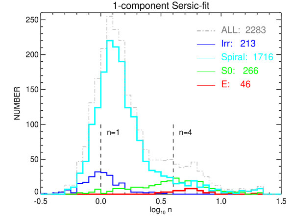
Figure 32: Histogram of Sérsic-index $n$ in 1-component Sérsic-fits. Dashed line indicates the whole S⁴G sample, after elimination of 61 galaxies due to bad image quality, bright nearby star etc. Additionally, for 8 galaxies the decomposition failed to converge ($n=20$ in the plot). The main morphological types are shown separately with different colors: Ellipticals ( $T<-3$), S0s ($-3\leq T\leq 0$), Spirals ($0<T<10$), and Irregulars ($T=10$). Additionally there are 8 galaxies without classification ($T=99$; the median value of their $n=2.3$), and 34 dwarf galaxies ($T=11$; median $n=1.3$) which are not shown. The Hubble stage $T$ is from the mid-IR morphological classification by Buta et al. (2014). The vertical dashed lines indicate the values $n=1$ and $n=4$, corresponding to exponential and de Vaucouleurs profiles, respectively.

Figure 32 displays the histogram of Sérsic index-values in the 1-component models. Galaxies are divided into three bins according to their mid-IR Hubble type (E with $T\leq-4$, S0 with $-3\leq T\leq 0$, spiral with $1\leq T\leq 9$, and irregulars $T=10$). Clearly, the distribution of galaxies peaks at $n\approx 1-2$, with a broad tail to larger values of $n$. There is also a secondary peak close to $n\approx 4$ (corresponds to a de Vaucouleurs profile), but this is not very prominent. The overall distribution reflects the nearly exponential profiles of many late type spirals, which dominate the $S^{4}G$ sample. For irregulars, the distribution peaks at $n\approx 1$. For S0’s, the distribution is much broader. The distributions remain essentially the same for less inclined galaxies, for example if the sample is limited to those with apparent $b/a>0.5$.

5.3 Multi-component decompositions

For multi-component decompositions the tabulation is more complicated, as model components/functions vary from one galaxy to another. Also, the same function can be used to describe different structure components in different galaxies. We have decided to present the multi-component parameters in two different formats, one that is compact and easily human-readable, another more suited to automatic reading. In the first format (Table 7) the first entry for each galaxy indicates the used model and the number of components. The next lines, for each component included in the model, indicate the physical interpretation of the component (B, D (or Z), bar, N), and the GALFIT function used (sersic,  expdisk, edgedisk, ferrer2, psf), followed by the component parameters. The Table caption specifies which parameters are listed for each function. The other table (available via IRSA and P4 web page) lists for each galaxy all possible components and their parameters: empty values indicate that this component was not included in the decomposition of this galaxy.

The $S^{4}G$ sample contains 358 galaxies which were considered to be close to an edge-on view and are excluded from further analysis in paper 2. Also, 26 are elliptical systems, modeled with a single Sérsic function. This leaves 1855 moderately inclined disk systems. As discussed in Section 3 there are over 20 different combinations of functions/components used in the final models, so that there is a need to group the decompositions in to major categories. A natural approach is to base this grouping on whether the decomposition model has a bulge component. Because the bulge can be modeled either with a “sersic” or “psf” component, depending on its apparent size, we have two categories, BD and ND models, respectively. When there is no trace of a bulge, the system can be either a single disk (D), possess a bar-like component (Dbar), or contain both inner and outer disk components (DD).

The numbers and relative fractions of galaxies in these categories as a function of Hubble type are shown in Fig. 33. Here the mid-IR classification from Buta et al. (2014) is followed. Apparently the relative fraction of BD-models decreases gradually towards the late-type spirals. However, taking into account that most of the ND models describe small bulges (support for this claim is given in paper 2), indicates a much smoother distribution of galaxies with bulges, dropping rapidly only above $T\sim 5$. The fact that ND models cover a relatively large range of Hubble types, including S0s, is quite interesting because it indicates that S0s can possess very small bulges. This is in agreement with Laurikainen et al. (2010), where the same conclusion was made based on decompositions of NIRS0S data. The result is consistent with the idea that at least some S0s might be former late-type spirals with small bulges, devoid of gas, following quenching of star formation. A very small $B/T$ ratio in an early-type spiral has also been reported also by Kormendy & Barentine (2010). Another interesting feature in Fig 33 is that many galaxies that lack bulges, can still have bars. These Dbar galaxies peak at Hubble types $T=7$. Beyond $T=9$ they are replaced with single disks, becoming almost the sole type of models for irregulars (T=10). The DD-models are most common (about 10%) for $T=9$.

Finally, Fig. 34 gives examples of galaxies in these major categories, indicating the model components for 4 low mass and 4 large mass systems in each category. For BD and ND categories the barred and non-barred models are also distinguished. Note that ’barred’/’non-barred’ refers here to whether or not a bar-component was included to the the final decomposition model, not to any morphological classification; for example a non-barred BD model has been adopted for NGC 5985, which has a SAB family classification (see Fig. 33). A detailed comparison to Buta et al. (2014) classification will be presented in paper 2.

Table 5: Summary of decomposition quality flags

Quality	#	#($\geq$quality)	1-component	Multi-component	Disk $\mu_{0}$ and $h_{r}$
1	31		-	-	-
2	44	2321	uncertain	-	-
3	61	2277	ok	uncertain	-
4	406	2216	ok	ok	uncertain (or z)
5	1810	1810	ok	ok	ok

Note. — Quality flags (1-5) assess the reliability of decomposition parameters. The second column indicates the number of galaxies in each class, while the third column indicates the number of galaxies with decomposition parameters of this or better quality.

Table 6: Parameters of 1-component Sérsic fits

Identification	Comment	mag	q	PA	$n$	$R_{e}$
ESO011-005		14.52	0.231	43.46	1.329	18.61
ESO012-010		13.31	0.493	156.97	1.592	56.38
ESO012-014		14.67	0.411	23.92	0.884	47.35
ESO013-016		12.75	0.508	168.64	1.314	38.85
ESO015-001		14.39	0.357	110.22	1.131	34.34
ESO026-001		12.52	0.689	58.26	3.126	62.93
ESO027-001		10.75	0.765	74.38	5.423	96.07
…
UGC12856		14.04	0.316	18.48	1.339	41.22
UGC12857		12.99	0.195	33.50	1.316	19.09
UGC12893		13.58	0.861	94.74	1.179	33.55

Note. — Comment indicates cases where no fit was made, fit failed to converge, or its parameters are not reliable. $mag$ is the the total magnitude, $q$ is the axial ratio and $PA$ the position angle of elliptical isophotes, $n$ is the Sérsic index and $R_{e}$ the effective radius (in arcsec).

Table 7: Parameters of final multicomponent decompositions

#1	ESO011-005	_bz	NCOMP=2	quality=4
	B	sersic	0.571	14.822	0.354	40.447	48.937	3.001
	Z	edgedisk	0.429	20.912	43.902	9.764	2.955
#2	ESO012-010	_dbar	NCOMP=2	quality=5
	D	expdisk	0.944	13.445	0.458	-33.795	33.953	23.095
	BAR	ferrer2	0.056	22.177	0.390	24.245	21.141
#3	ESO012-014	_dbar	NCOMP=2	quality=4
	D	expdisk	0.835	14.795	0.420	31.032	33.152	24.393
	BAR	ferrer2	0.165	24.704	0.249	11.102	83.009
…
#2352	UGC12893	_bd	NCOMP=2	quality=5
	B	sersic	0.021	17.826	0.786	102.674	6.559	0.515
	D	expdisk	0.979	13.617	0.869	87.208	20.150	22.134

”

Note. — The first row for each galaxy is the running number (1-2352). The second row gives the galaxy name, the type of final decomposition model (coded to all output file names together with underscore-prefix), the number of components in the model, and the quality flag. If no final decomposition was made (quality= 1 or 2) then for this galaxy we set type=’-’ and NCOMP=0. The next NCOMP entries give: (1) the physical interpretation of the component (B-bulge, D-disk, Z-edge-on disk, BAR-bar, N-unresolved central component), (2) the GALFIT function used for it, and (3) the component’s relative fraction of the total model flux. The next entries depend on the GALFIT function. For sersic they are: $mag,q,PA,n,R_{e}$, for expdisk: $mag,q,PA,h_{r}$, for edgedisk: $\mu_{0},PA,h_{r},h_{z}$, for ferrer2: $\mu_{0},q,PA,R_{bar}$, and for psf: $mag$. Here $mag$ is the total 3.6 $\mu$m AB magnitude, $\mu_{0}$ is the central surface brightness in mag/arcsec² (face-on brightness for expdisk and edgedisk, sky brightness for ferrers2), $R_{e},h_{r},h_{z}$ are in arcsecs. All decompositions assume a fixed common center for all components and elliptical isophotal shape, constant over radius. If there is an (outer) disk, its $q$ and $PA$ are kept fixed to those in Table I.

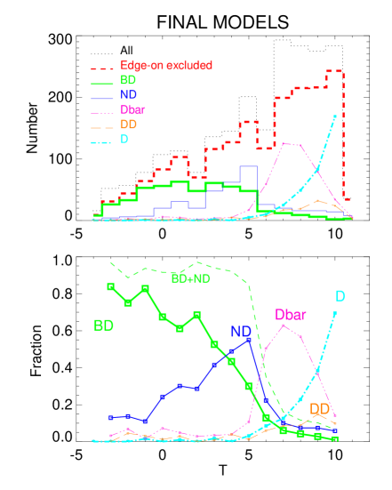
Figure 33: Distribution of final decomposition model categories as a function of mid-IR Hubble stage from Buta et al (2014; the half-integer values of T have been rounded before binning, see caption of Fig. 27). In the upper panel the distribution of the original S⁴G sample (dotted histogram), and of galaxies with final models (red dashed line histogram; excluding the edge-on galaxies). The green histogram is the distribution of models where both ’bulge’ and ’disk’ components where identified (BD). This is also the subsample used in Section 4.4 when comparing automatic 2-component and final multi-component decompositions. The dark blue line shows the distributions for models with both ’nucleus’ and ’disk’ (excludes those with ’bulge’) (ND). The three other lines are for models with neither ’bulge’ nor ’nucleus’: ’Dbar’ stands for models where a Ferrers-bar was included (together with one or more ’expdisk’ components), ’DD’ stands for models with inner and outer disks, while ’D’ stands for a single ’expdisk’ model. In the lower panel the relative fractions of different models are plotted, normalized to the total number of non edge-on models (red dashed curve curve in the upper panel). Here ’BD’ and ’ND’ include both models with/without ’bar’: for clarity, these are not shown separately as the differences in the distributions are small.

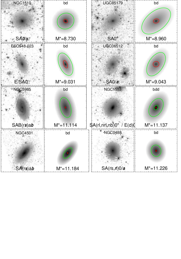
Figure 34: a) Examples of different main types of final decomposition models. Four low mass and four large mass galaxies of each type are displayed. The left frames display the 3.6 $\mu$m image, with fixed AB surface brightness range [18,27], while the right indicates the model components: the semi-major axis corresponds to $2R_{\rm eff}$ of the component. The labels in the left frame indicate the galaxy name and the Buta et al. (2014) mid-IR classification; in the plots the Buta et al. underline notation is indicated with slanted characters. Labels in the right frames give the physical coding of the decomposition model components (same as used in the names of the decomposition files), and the $\log_{10}(M_{star})$ (stellar masses are from Muñoz–Mateos et al. 2014). The colors of the ellipses indicate the used functions: expdisk (green), sersic (red), ferrer2 (blue). Similar plots for all galaxies are given in the P4 web-page. In a) examples of BD models (have bulge & disk but no bar component) are displayed.

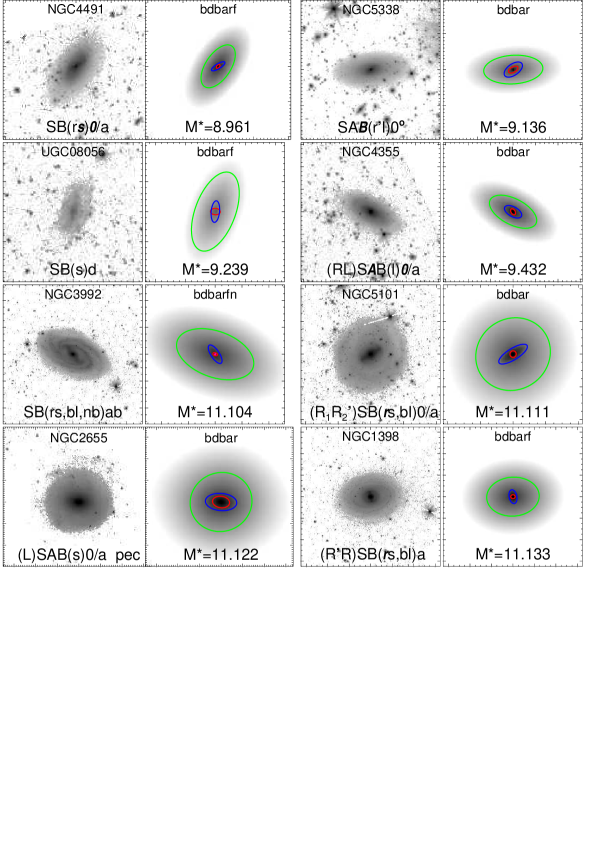
Figure 34b: Examples of BDbar decomposition models (bulge & disk with a bar component). ’barf’ indicates that the length of the Ferrers bar was fixed in the decompositions.

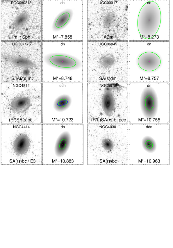
Figure 34c: Examples of ND decomposition models (nucleus & disk, no bar). The central component (unresolved in decomposition) is indicated with a red dot.

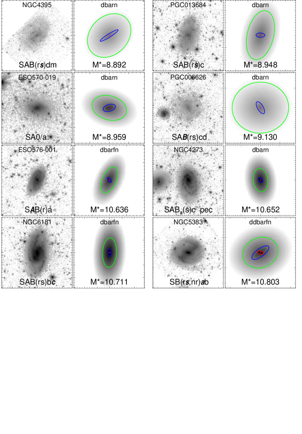
Figure 34d: Examples of NDbar decomposition models (nucleus & disk, with a bar).

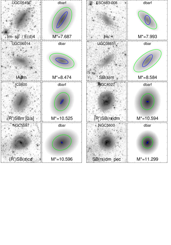
Figure 34e: Examples of Dbar decomposition models (disk & bar).

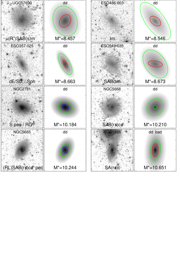
Figure 34f: Examples of DD decomposition models (two disk components).

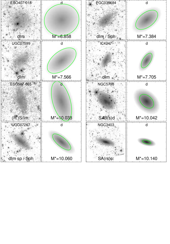
Figure 34g: Examples of D decomposition models (single disk).

6 Summary and Conclusions

Two-dimensional multi-component decompositions, using GALFIT3.0, have been performed at 3.6 $\mu$m wavelength for the complete S⁴G sample (2352 galaxies). Reliable decompositions were possible for 2277 galaxies. Quality flags are given for each galaxy based on our confidence on the model parameters. The main goal of the decompositions was to estimate the structural parameters of the bulges and disks in a reliable manner, which dictated our decomposition strategy. Most importantly, a bar-component was included in the decomposition model whenever present, to prevent its light from biasing the derived bulge and disk parameters. For the same reason, the models sometimes included a central point source and additional disk components. However, no attempt was made to match the detailed shape or length of the bar.

We present automated single Sérsic, 2-component bulge-disk (Sérsic + exponential) decompositions, and human-supervised, individually checked multi-component models. In the final multi-component models, a maximum of four structural components are fit: bulge (Sérsic), disk (exponential), bar (modified Ferrers), and the nucleus (PSF). Different combinations of component functions were used. For example, in some barred galaxies it was convenient to fit the underlying disk with two different functions. As a first step, we estimated the sky background levels, derived the orientation parameters with ellipse fitting, and edited the masks to eliminate foreground stars and image defects. In general we found an excellent agreement with the independent P3 measurements (Muñoz–Mateos et al. 2014).

The uncertainties related to the sky background, the adopted PSF-function, and to the treatment of sigma-images were tested. The decomposition data are released in IRSA, and in the P4 web-page, where the decomposition models, the ellipse fitting, and sky background determinations are illustrated. The IDL-based tool (GALFIDL) used in visualization of GALFIT decompositions is also available on the web pages. Besides the decomposition output files, all input files needed in re-doing the decompositions are given in IRSA. All of this provides the possibility to refine the pipeline models for the needs of specific scientific goals.

In particular, such refined models will be needed for early-type galaxies which often contain more structures than handled by current pipeline decompositions: for ellipticals such structures include nuclear point sources (Lauer 1985; Côté et al. 2006) and inner disk structures (Kormendy & Bender 1996, Buta et al. 2014; modeled in Kormendy & Barentine 2010, Weinzirl et al. 2014); for S0s and early-type spirals the various lens structures (Kormendy 1979; Laurikainen et al. 2009) should be accounted for, including the barlens components (Laurikainen et al. 2011) recently identified as the more face-on counterparts of boxy/peanut bulges seen in nearly edge-on galaxies (Laurikainen et al. 2014; Athanassoula et al. 2014). Such refined models become particularly important with the ongoing extension of S⁴G data to include 465 additional gas-poor early-type galaxies (Sheth et al. 2013), which were not part of the original sample which contained only galaxies with emission line velocity measurements.

The main results are the following:

(1) Automatic single Sérsic fits. The Sérsic indexes peak at $n\sim$1.5, having only a minor peak at $n\sim$4, reflecting the fact that a large majority of the sample galaxies are spirals with extended disks.

(2) Automatic 2-component bulge-disk decompositions: Such decompositions would suggest a large difference in the parameters of the bulges between barred and non-barred galaxies. Since this is an artifact caused by the inadequate decomposition model, we strongly caution against using simple bulge-disk decompositions for barred galaxies.

(3) Final multi-component decompositions. In contrast to 2-component models, in our final models the differences in bulge parameters between barred and non-barred galaxies disappear, leading to the values of Sersic $n\sim 1-2$ for bulges in both types of galaxies. It means that if bars are not included in the fit, the flux of the bar is erroneously mixed with the bulge flux. This conclusion is consistent with several previous studies using a similar multi-component decomposition approach.

(4) Small bulges containing at most a few percent of the galaxy flux at 3.6 $\mu$m appear in a large range of Hubble types, including S0s. This is in agreement with Laurikainen et al. (2010) where a similar result was obtained in near-IR.

(5) At intermediate Hubble types (T=5-7) the very small bulges gradually disappear but the galaxies can still be either barred or non-barred. At the very end of the Hubble sequence pure disks become dominant.

A detailed analysis of the properties of bulges, disks, and bars, as a function of morphological type, and other overall properties (galaxy mass and global color) will be presented in forthcoming paper (Paper 2 in preparation).

7 Acknowledgments

H. Salo, E. Laurikainen, and S. Comeron acknowledge the Academy of Finland for support. J. Laine was supported by the Väisälä Foundation Grant. E.A. and A.B acknowledge the CNES (Centre National d’Etudies Spatiales - France) for financial support. The authors also acknowledge support from the FP7 Marie Curie Actions of the European Commission, via the Initial Training Network DAGAL under REA grant agreement number 289313.

We thank J. Janz for discussions and for help with the initial preparation of the web-pages. We also thank the Spitzer IRAC Instrument Support Team for its help with the sigma-images.

Appendix A Appendix: Decomposition pipeline products in IRSA

The results of pipeline 1-component and final multi-component decompositions are available via the IRSA database. For each galaxy, decomposition output parameters (outgal-file), and input fits-files are given. The user can refine/improve the given multi-component models by including more components or by utilizing additional GALFIT options for the component functions.

------------------------------------------
1) Input data for GALFIT decompositions
------------------------------------------

IDE is the galaxy designation (e.g. NGC1097)

fits-files:
  IDE.phot.1_nonan.fits     = 3.6 micron image used in decompositions,
                              Bad pixel values (NaN’s) removed
                              header modified to make GALFIT work correctly
  IDE.1.finmask_nonan.fits  = corresponding mask-file
  IDE.phot.1_sigma.fits_ns  = -"- sigma-image
  PSF-1.composite.fits      = PSF-image

------------------------------------------
2) Output from GALFIT decompositions
------------------------------------------

a) ascii-files:

  IDE_onecomp.outgal       =    Automatic best fit parameters for 1-component S\’ersic model
  IDE_twocomp.outgal       =    -"-  for 2-component sersic+expdisk (or sersic-edgedisk) fit
  IDE_MODEL.outgal         =    Final decomposition model with up to 4 different components

  IDE is the galaxy designation (e.g. NGC1097)
  MODEL-string identifies the components included in the final multi-component model:

        ’b’    indicates bulge-component
        ’d’    indicates disk -"-
        ’bar’  indicates non-axisymmetric structure, mainly bars
               ’barf’ -> length of the bar was fixed in the decompositions
        ’n’    indicates nucleus (or nonresolved bulge)
        ’z’    indicates edge-on disk

         e.g. "NGC1415_bdbar"  -> bulge+disk+bad final decomposition model

  These outgal-files contain the decomposition output parameters
  Together with the input fits-files, the user can immediately repeat/refine the decompositions
  starting from the outgal-file (e.g. outgal -o1 NGC1415_bdbar.outgal   -> re-creates the decomposition)


b) fits-file (for the FINAL model)

  IDE_MODEL.outgal_subcomps.fits      Final decomposition output images:
                                      extension 1 =  OBS image
                                      extension 2,3,4... = model components
                                      File header contains also final decomposition parameters.

c) jpg-files (for the FINAL MODEL)

   IDE_MODEL.outgal_profile.jpg        Decomposition model compared with observations:
                                       - shows surface brightness at each image pixel vs distance from galaxy center
                                         Observed image, model image, and model components displayed separately
                                       - Collects also decomposition input & output parameters
                                         Labels indicate relative contribution of model components

   IDE_MODEL.outgal_residual.jpg       Model-observation comparisons:
                                         upper row: clipped 3.6 micron image, masked image
                                         lower row: model image, OBS-MODEL residual
   ΨΨΨΨ
   IDE_MODEL.outgal_1dprof.jpg         Decomposition model profiles compared with observations:
                                       - shows surface brightness as a function of isophotal semi-major axis,
                                         comparing IRAF ellipse fits to the observed image and to the
                                         model image (using isophotes of the observed image)
ΨΨΨΨΨ

   IDE_MODEL.outgal_components.jpg     Schematic plot of model components:
                                       - Upper row: Observed image and model image, with different model
                                         components marked: colors correspond to profile plots, and the semimajor-axis
                                         of the ellipse is 2 times the effective radius of the components
                                       - Lower row: same as upper row, except projected to the disk plane
                                         (assuming zero-thickness). Empty in case on edge-on final model.

====================================================================================================================
  The final decomposition models, as well as various intermediate steps involved, are illustrated in the web-page
  http://www.oulu.fi/astronomy/S4G_PIPELINE4/MAIN
====================================================================================================================

Appendix B Appendix: Decomposition Pipeline web-pages

The input data used in decompositions, the various steps of the decomposition pipeline, and the final decomposition results are illustrated on the Pipeline 4 web site

http://www.oulu.fi/astronomy/S4G_PIPELINE4/MAIN

The web site consists of three layers of pages:

1) Main page

2) Index pages

3) Decomposition pages

The main page gives full instructions regarding the contents of the pages, followed by an alphabetical list of all 2352 galaxies in the original sample Clicking on any of the galaxy names opens a corresponding index page, with contains information for 100 galaxies, near and including the chosen galaxy (Fig. 41).

The icons in the index page indicate the data available for each galaxy

1) P1 image mosaic

2) clipped P1 image, with mask

3) clipped P1 image

4) Deprojected image

5) Elliptical isophote profiles

6) Galaxy center/sky background plots

What decompositions available:

7) 1-component Sérsic-model (icon shows residual plot)

8) Final-model (icon shows residual plot)

9) Final-model (icon shows model components)

An empty icon signifies no data/decomposition model, for instance if the galaxy was discarded from further analysis because of a nearby bright star, etc. In particular, the absence of a final model indicates that the galaxy was considered too problematic to fit reliably (e.g. closely interacting, very peculiar or warped).

Clicking on the galaxy name links to its decomposition page (Fig. 42), which summarizes the mask, ellipse fitting, sky background, and galaxy center determinations, as described in Section (2.2).

In addition, the pages display for all three types of models (1-component Sérsic model, 2-component bulge/disk model , final multi-component model) the

2D profile plot

Residual plot

1D profile plot

Model-components plot

Again, clicking on the plots displays the full size plots (Figs. 43 44, 45, 46).

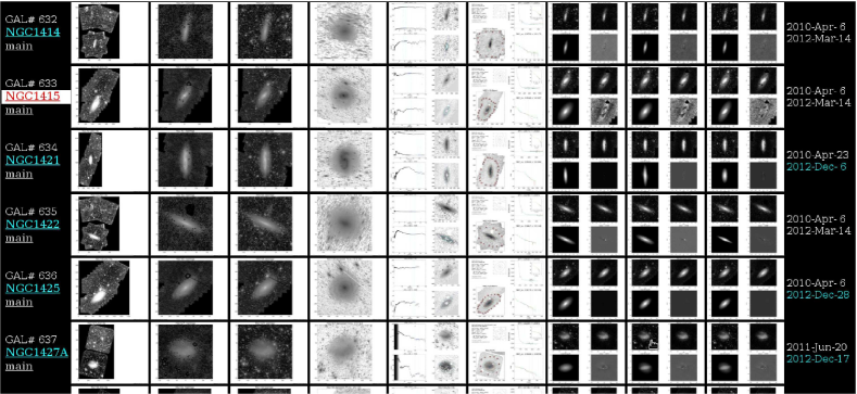
Figure 41: Screenshot of Pipeline 4 index page.

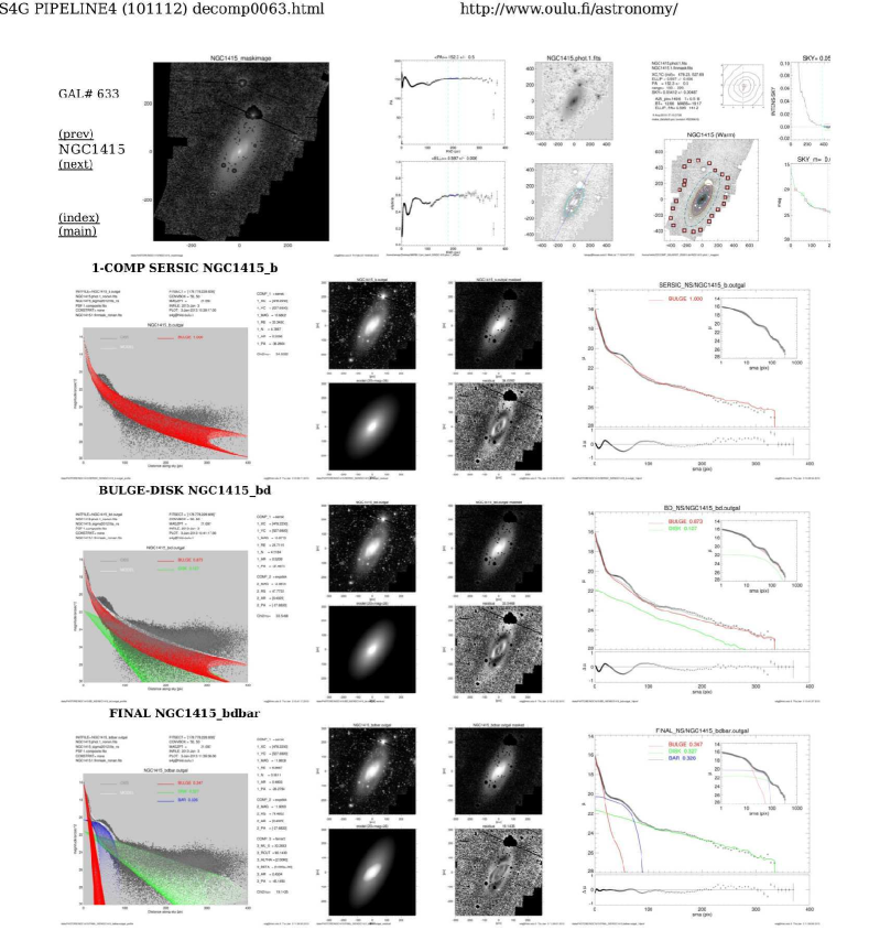
Figure 42: Screenshot of various decomposition models for this particular galaxy. Clicking on the image icons opens the enlarged image.

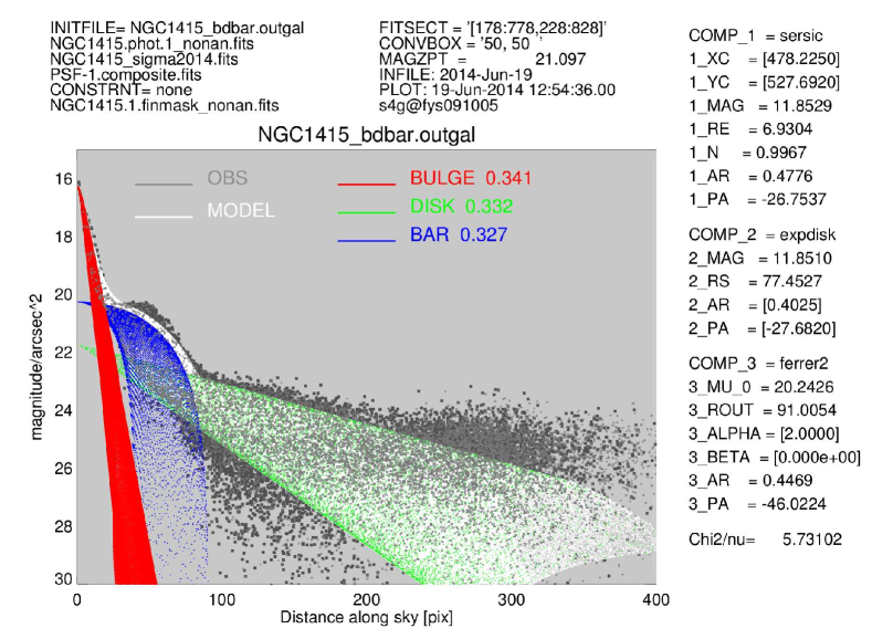
Figure 43: Final pipeline decomposition for NGC 1415. The decomposition includes bulge, disk, and bar components, indicated by different colors. The numbers after the labels indicate the relative fraction of light in each component. This 2D-profile indicates the brightness of each pixel versus its distance from the galaxy center. The frame also collects the names of the input data files and the final GALFIT decomposition parameter values.

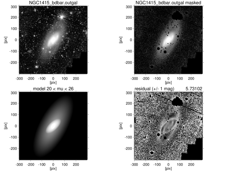
Figure 44: Final pipeline decomposition for NGC 1415, corresponding to Fig. 43. The upper frames show the observed, clipped and sky-subtracted image (left) and the corresponding masked image (right). The lower frames display the model image (left), and the observed-model residual image (gray scale covers $\pm 1$ mag).

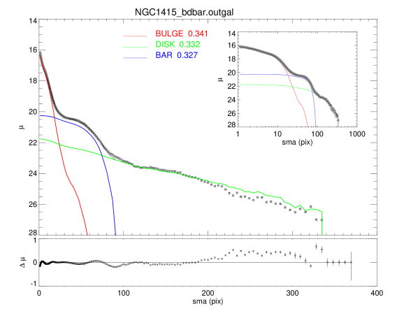
Figure 45: One dimensional profiles corresponding to Fig. 43. The symbols indicate the azimuthally averaged surface brightness as a function of semi-major axis, obtained with IRAF ellipse-routine. The curves indicate the azimuthally averaged profiles of the model components, using the same isophotes.

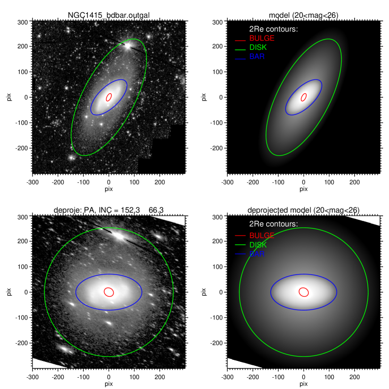
Figure 46: Illustration of the model components corresponding to Fig. 43. The upper left shows the observed image, together with superposed ellipses illustrating the various components of the final model: the size of the ellipse corresponds to 2 effective radii, the orientation corresponds to the components’ axial ratio and PA. In the upper right, the same but showing the model image. The lower frames are similar, except that the observed galaxy and the model have been deprojected, using the assumed disk orientation parameters.

References

- Athanassoula (2005) Athanassoula, E., 2005, MNRAS, 358, 1477
- (2)
- Athanassoula et al. (2014) Athanassoula, E., Laurikainen, E., Salo, H., & Bosma, A. 2014, arXiv:1405.6726
- Allen et al. (2006) Allen, P., Driver, S., Graham, A., Cameron, E., Liske, J., de Propris, R., 2006, MNRAS, 371, 2
- Athanassoula et al. (1990) Athanassoula, E., Morin, S., Wozniak, H., Puy, D., Pierce, M., Lombard, J., Bosma, A., 1990, MNRAS, 245, 130
- Bacos & Trujillo (2012) Bakos, J., Trujillo, I., 2012, MSAIS, 25, 21
- Barazza et al. (2008) Barazza, F., Jogee, S., Marinova, I., 2008, ApJ, 675, 1194
- Bertin & Arnouts (1996) Bertin, E., Arnouts, S. 1996, A&AS, 117, 393
- Buta et al. (2010) Buta, R. J., Sheth, K., Regan, M., et al. 2010, ApJS, 190, 147
- Buta et al. (2014) Buta R. J. et al., 2014. Submitted to ApJS
- Combes & Sanders (1981) Combes, F., & Sanders, R. H. 1981, A&A, 96, 164
- Cameron et al. (2009) Cameron, E., Driver, S., Graham, A., Liske, J., 2009, ApJ, 699, 105
- Cappellari et al. (2013) Cappellari, M., McDermid, R., Alatalo, K., Blitz, L., Bois, M., Bournaud, F., Bureau, M., Crocker, A., Davies, R., Davis, T. and 14 coauthors, 2013, MNRAS, 432, 1862
- Comerón et al. (2011) Comerón, S., Elmegreen, B. G., Knapen, J. H., Sheth, K., Hinz, J. L., Regan, M. W., Gil de Paz, A., Muñoz-Mateos, J.-C., Menéndez-Delmestre, K., Seibert, M., Kim, T., Mizusawa, T., Laurikainen, E., and 10 co-authors, 2011, 738, L17
- Comerón et al. (2012) Comerón, S., Elmegreen, B. G., Salo, H., Laurikainen, E., Athanassoula, E., Bosma, A., Knapen, J. H., Gadotti, D. A.,Sheth, K. and 10 coauthors, 2012, ApJ, 759, 98
- Comerón et al. (2014) Comerón, S., Elmegreen, B. G., Salo, H., et al. 2014, arXiv:1409.0466
- Côté et al. (2006) Côté, P., Piatek, S., Ferrarese, L., et al. 2006, ApJS, 165, 57
- Courteau et al. (2007) Courteau S., Dutton A. A., van den Bosch F. C., MacArthur L. A., Dekel A., McIntosh D. H., Dale D. A., 2007, ApJ, 671, 203
- de Souza et al. (2004) de Souza, R. E., Gadotti, D. A., & dos Anjos, S. 2004, ApJS, 153, 411
- de Vaucouleurs et al. (1991) de Vaucouleurs, G., de Vaucouleurs, A., Corwin, Jr., H. G., et al. 1991, (RC3)
- Driver et al. (2006) Driver, S., Allen, P., Graham, A., Cameron, E., Liske, J., Ellis, S., Cross, N., De Propris, R., Phillipps, S., Couch, W., 2006, MNRAS, 368, 414
- Driver et al. (2013) Driver, S., Robotham, A., Bland-Hawthorn, J., Brown, M., Hopkins, A., Liske, J., Phillipps, S., Wilkins, S., 2013, MNRAS, 430, 2622
- Draine & Lee (1984) Draine, B., Lee, H., 1984, ApJ, 285, 89
- Erwin, Beckman & Pohlen (2005) Erwin, P., Beckman, J., Pohlen, M., 2005, ApJ, 626, L81
- Eskridge et al. (2002) Eskridge, P. B., Frogel, J. A., Pogge, R. W., Quillen, A. C., Berlind, A. A., Davies, R. L., DePoy, D. L., Gilbert, K. M., Houdashelt, M. L., Kuchinski, L. E., and 5 coauthors, 2002, ApJS, 143, 73
- Fisher (2006) Fisher D., 2006, ApJ, 642, 17
- Fisher & Drory (2010) Fisher, D. B., & Drory, N. 2010, ApJ, 716, 942
- Freeman (1970) Freeman K., 1970, ApJ, 160, 811
- Gadotti (2001) Gadotti, D. A., dos Anjos, S., 2001, AJ, 122, 1298
- Gadotti (2008) Gadotti, D. A. 2008, MNRAS, 384, 420
- Gadotti (2009) Gadotti D. A., 2009, MNRAS, 393, 1531
- Gadotti (2011) Gadotti D. A., 2011, MNRAS, 415, 3308
- Graham & Worley (2008) Graham A., Worley C.C., MNRAS, 388, 1708
- Gutiérrez et al. (2011) Gutiérrez L., Erwin P., Aladro R., Beckman J. E., 2011, AJ, 142, 145
- Häußler (2013) Häußler, B., Bamford, S., Vika, M., Rojas, A., Barden, M., Kelvin, L., Alpaslan, M., Robotham, A., Driver, S., Baldry, I., and 6 coauthors, 2013, MNRAS, 430, 330
- Huang et al. (2013) Huang, S., Ho, L., Peng, C., Li, Z. Barth, A., 2013, ApJ, 766, 47
- Janz et al. (2014) Janz, J., Laurikainen, E., Lisker, T., et al. 2014, ApJ, 786, 105
- Jedrzejewski (1987) Jedrzejewski R. I., 1987, MNRAS, 226, 747
- Lackner & Gunn (2012) Lackner, C., Gunn, J., 2012, MNRAS, 421, 2277
- Kim et al. (2014) Kim, T., Gadotti, D. A., Sheth, K., et al., 2014, ApJ, 782, 64
- Knapen et al. (2014) Knapen, J. H., Erroz-Ferrer, S., Roa, J., et al. 2014, A&A, 569, A91
- Kormendy (1979) Kormendy, J. 1979, ApJ, 227, 714
- Kormendy (1982) Kormendy, J. 1982, ApJ, 257, 75
- Kormendy (1993) Kormendy, J. 1993, Galactic Bulges (IAU Symposium 153), p. 209
- Kormendy & Bender (1996) Kormendy, J., & Bender, R. 1996, ApJ, 464, L119
- Kormendy et al. (2009) Kormendy, J., Fisher, D. B., Cornell, M. E., & Bender, R. 2009, ApJS, 182, 216
- Kormendy & Barentine (2010) Kormendy, J., Barentine J.C., 2010, ApJ, 715, 176
- Kormendy & Bender (2012) Kormendy, J., & Bender, R. 2012, ApJS, 198, 2
- Kormendy & Kennicutt (2004) Kormendy, J., & Kennicutt, R. C., Jr. 2004, ARA&A, 42, 603
- Laine et al. (2014) Laine, J., Laurikainen, E., Salo, H., et al. 2014, MNRAS, 441, 1992
- Landsman (1993) Landsman 1993, in Astronomical Data Analysis Software and Systems II, A.S.P. Conference Series, Vol. 52, ed. R. J. Hanisch, R. J. V. Brissenden, and Jeannette Barnes, p. 246.
- Lauer (1985) Lauer, T. R. 1985, ApJ, 292, 104
- Laurikainen et al. (2005) Laurikainen, E., Salo, H., Buta, R., 2005, MNRAS, 362, 1319
- Laurikainen et al. (2006) Laurikainen, E., Salo, H., Buta, R., Knapen, J., Speltincx, T., Block, D. L., 2006, AJ, 132, 2634
- Laurikainen et al. (2007) Laurikainen, E., Salo, H., Buta, R., & Knapen, J. H., 2007, MNRAS, 381, 401
- Laurikainen et al. (2009) Laurikainen, E., Salo, H., Buta, R., & Knapen, J. H., 2009, ApJ, 692, 34
- Laurikainen et al. (2010) Laurikainen, E., Salo, H., Buta, R., Knapen, J. H., Comerón, S., 2010, MNRAS, 405, 1089
- Laurikainen et al. (2011) Laurikainen, E., Salo, H., Buta, R., & Knapen, J. H. 2011, MNRAS, 418, 1452
- Laurikainen et al. (2014) Laurikainen, E., Salo, H., Athanassoula, E, Bosma, A, Herrera-Endoqui, M. 2014, MNRAS, 444, L80
- Martín-Navarro et al. (2012) Martín-Navarro, I., Bakos, J., Trujillo, I., et al. 2012, MNRAS, 427, 1102
- Meidt et al. (2012) Meidt, S. E., Schinnerer, E., Knapen, J. H., et al. 2012, ApJ, 744, 17
- Melvin et al. (2014) Melvin, T., Masters, K., Lintott, C., et al. 2014, MNRAS, 438, 2882
- Muñoz-Mateos et al. (2013) Muñoz-Mateos, J. C., Sheth, K., Gil de Paz, A., et al. 2013, ApJ, 771, 59
- Muñoz–Mateos et al. (2014) Muñoz–Mateos J. C. et al., 2014, ApJS, submitted
- Nair et al. (2010) Nair, P., Abraham, R., 2010, ApJ, 714, 260
- Pahre et al. (2004) Pahre, M. A., Ashby, M. L. N., Fazio, G. G., Willner, S. P. 2004, ApJS, 154, 235
- Peletier et al. (2012) Peletier, R., Kutdemir, E., van der Wolk, G., Falcón-Barroso, J., Bacon, R., Bureau, M., Cappellari, M., Davies, R., de Zeeuw, P., Emsellem, E., and 8 coauthors, 2012, MNRAS, 419, 2031
- Peng et al. (2002) Peng, C., Ho, L., Impey, C. Rix, H., 2002, AJ, 124, 266
- Peng et al. (2010) Peng, C., Ho, L., Impey, C., Rix, H., 2010 AJ, 139, 2097
- Pohlen & Trujillo (2006) Pohlen M., Trujillo I., 2006, A&A, 454, 759
- Querejeta et al. (2014) Querejeta, M., Meidt, S. E., Schinnerer, E., et al. 2014, arXiv:1410.0009
- Regan et al. (2014) Regan, M. et al., 2014, in prep.
- Rest et al. (2001) Rest, A., van den Bosch, F. C., Jaffe, W., et al. 2001, AJ, 121, 2431
- Sellwood (2008) Sellwood, J.A., 2008, in ’Dynamical Evolution of Disk Galaxies’, Astronomical Society of the Pacific Conference Series 396, eds. . G. Funes & E. M. Corsini
- Sheth (2008) Sheth, K. 2008 et al ApJ675, 1141
- Sheth et al. (2010) Sheth K., et al., 2010, PASP, 122, 1397
- Sheth et al. (2013) Sheth, K., Armus, L., Athanassoula, E., et al. 2013, Spitzer Proposal, 10043
- Tasca & White (2011) Tasca, L. A. M., & White, S. D. M. 2011, A&A, 530, A106
- van der Kruit & Searle (1981) van der Kruit, P. C., Searle L., 1981 A&A, 95, 105
- van der Wel (2008) van der Wel, A. 2008, ApJ, 675, L13
- Weinzirl et al. (2009) Weinzirl, T., Jogee, S., Khochfar, S., Burkert, A., Kormendy, J. 2009 ApJ, 696, 411.
- Weinzirl et al. (2014) Weinzirl, T., Jogee, S., Neistein, E., et al. 2014, MNRAS, 441, 3083
- Zaritsky et al. (2013) Zaritsky, D., Salo, H., Laurikainen, E., et al. 2013, ApJ, 772, 135