Sufficient conditions for the additivity of stall forces generated by multiple filaments or motors

Abstract

Molecular motors and cytoskeletal filaments work collectively most of the time under opposing forces. This opposing force may be due to cargo carried by motors or resistance coming from the cell membrane pressing against the cytoskeletal filaments. Some recent studies have shown that the collective maximum force (stall force) generated by multiple cytoskeletal filaments or molecular motors may not always be just a simple sum of the stall forces of the individual filaments or motors. To understand this excess or deficit in the collective force, we study a broad class of models of both cytoskeletal filaments and molecular motors. We argue that the stall force generated by a group of filaments or motors is additive, that is, the stall force of $N$ number of filaments (motors) is $N$ times the stall force of one filament (motor), when the system is in equilibrium at stall. Conversely, we show that this additive property typically does not hold true when the system is not at equilibrium at stall. We thus present a novel and unified understanding of the existing models exhibiting such non-addivity, and generalise our arguments by developing new models that demonstrate this phenomena. We also propose a quantity similar to thermodynamic efficiency to easily predict this deviation from stall-force additivity for filament and motor collectives.

I Introduction

Molecular motors (such as kinesin, dynein and myosin) and cytoskeletal filaments (such as actin and microtubule) are abundantly present in eukaryotic cells and are responsible for important cellular functions. Cytoskeletal filaments give structural stability to the cell and act as tracks along which molecular motors move and facilitate intra-cellular transportation Lodish2007 ; nelsonbook ; Alberts2002 ; Hirokawa2010610 ; Vale2003467 ; crossNatReav2014 . Many researchers have studied the dynamics of single filaments and single motors in great detail using experimental and theoretical tools bustamante2001acr ; molloy1995nature ; fisher1999 ; kolomeisky2007 ; kolomeisky2013jp ; dcPR2013 ; clancy2011nsmb ; tripti2013 ; veigel2011nrmcb ; Ranjith2009 ; Desai_Mitchison_MT:97 ; Mcintosh1998 ; hill:84-2 ; schnitzer2000nat . However, inside a cell, molecular motors or cytoskeletal filaments work collectively most of the time to perform their biological tasks. For example, the dynamics of multiple actin filaments is responsible for lamellipodial protrusions during crawling of cells rafelski2004-73 ; schaus_performance_2008 . Similarly, microtubules work collectively to bring about segregation of chromosomes during mitosis KlineSmith2004317 . Many dynein motors attach to molecular cargo and generate force for cellular transportation efremov_delineating_2014 ; Mehta1999Nature , while myosin motors primarily work together to generate forces in stress fibres and muscle tissues. Hence, study of such systems, which are involved in a wide range of biological processes, requires understanding of the generation of collective force by multiple cytoskeletal filaments or motors doorn2000 ; levi_organelle_2006 ; lacostenjp2011 ; krawczykepl2011 ; Kierfeld:2013 ; dd2014 ; joanny2006prl ; CasademuntPRL2009 ; ambarish:2008 ; jacprost2008BJ ; demoulin_power_2014 ; Koster23122003 ; Leduc07122004 .

To understand collective force generation by polymerizing biofilaments, researchers typically resort to in vitro experiments in which biofilaments are polymerised either in the form of bundles or branched sheets against a barrier, which resists their motion by producing reaction forces Dogterom31101997 ; janson2004prl ; Kovar12102004 ; Laan01072008 ; Brangbour2011plos ; demoulin_power_2014 . One important focus of these studies is a quantity called the stall force, which is defined as the resisting force at which the mean growth velocity of the collection of filaments is zero, and is the maximum pushing force generated by these filaments.

A number of experiments on force generation by an assembly of biofilaments have been reported in the literature Dogterom31101997 ; McGrath2003329 ; Janson23062003 ; Kovar12102004 ; Marcy20042004 ; Prass11092006 ; Parekh2005NCB ; Footer2007 ; Laan01072008 ; Brangbour2011plos ; demoulin_power_2014 . In view of the overall content and objective of our paper we will focus only on the experiments related to single and parallel bundles of growing biofilaments. Experiments on single actin-filament are relatively rare due to experimental limitations created by the easy buckling tendency of a single actin filament. To the best of our knowledge, only one set of experiments has reported stall force for a single growing actin filament – a value of $\approx 1$pN Kovar12102004 . In another set of experiments on a few actin filaments growing in parallel, Footer et al. Footer2007 reported a collective stall force of $\approx 1$ pN, which is very similar to the load required to stall a single filament. In this experiment, the interpretation of filament cooperativity while pushing together against the barrier is, however, complicated by the fact that individual actin filaments may buckle before reaching their stall force, and hence, collectively the bundle may be unable to reach its full potential for force generation. On the other hand, in similar experiments performed on microtubules, researchers have found that the growth velocity of the filament growing against an immobile barrier decreases with increased resistance – from $1.2\mu$m per minute at zero load to $0.2\mu$m per minute at 4pN to 5pN force, which is the putative stall force in this case Dogterom31101997 . In another experiment based on microtubules, using optical tweezers, Laan et al. Laan01072008 report that stall forces of $2.7$pN, $5.5$pN and $8.1$pN are produced by groups of filaments. They interpreted this as containing one, two and three filaments, respectively. Hence, they concluded that stall force scales linearly with the number of filaments though there could be possible ambiguity in directly counting the number of filaments in the group.

On the theoretical and computational front, there are a number of very detailed models for understanding the force-velocity dynamics of a single biofilament Peskin_Oster:93 ; mogilner1999 ; kolomeisky2001bj ; zhang2011jbc , as well as a few that try to model the dynamics of multiple biofilaments doorn2000 ; kolomeiskyjcp2004 ; lacostenjp2011 ; krawczykepl2011 ; Kierfeld:2013 ; wang_load_2014 ; dd2014 ; dd2014-2 . Some of these theoretical studies have demonstrated that the stall force of multiple, non-interacting filaments without ATP/GTP dynamics, scales linearly with the number of filaments doorn2000 ; lacostenjp2011 ; Kierfeld:2013 ; krawczykepl2011 ; kolomeiskyjcp2004 . In contrast, a few other recent papers quite clearly report that inclusion of ATP/GTP hydrolysis can lead to either enhanced or reduced cooperativity in the maximum force generated by multiple growing filaments; the stall forces need not always scale with the number of filaments dd2014 ; dd2014-2 ; kolomeisky2015 ; aparna2015conf . In other words, the stall forces of individual filaments are non-additive in general, that is, the collective stall force produced by $N$ number of filaments (denoted by $f_{s}^{(N)}$) is not just a simple sum of individual stall forces of single filaments (i.e., $f_{s}^{(N)}\neq Nf_{s}^{(1)}$). It is quite intriguing as to why tweaking an internal variable (ATP/GTP) for an individual filament without actually changing any external interaction between the filaments can lead to this drastic change in their collective generation of force.

In studies similar to those on the biofilaments, the stall force for motors is defined by the resisting force at which the average velocity of the motors is zero. The experiments on molecular motor force generation mostly involve micro-sized dielectric particles and optical tweezers, by which a resisting force is applied on the moving motors, in order to measure their velocity response as a function of the resisting force SVOBODA1994773 ; Finer1994113 ; roopmallik2004 ; Takagi20061295 ; Wang1998902 ; visscher1999nat ; Mallik20052075 ; Jamison20102967 ; fallesen2011 ; Blehm26022013 ; Hendricks06112012 ; Rai2013172 . We briefly describe in the following text, a few examples that are relevant for our current study. Single molecule study of kinesin shows that kinesin is a strong molecular motor and generates maximum force of magnitude $\approx$ 5–8pN  SVOBODA1994773 ; visscher1999nat , whereas the stall force of certain variants of dynein is measured to be a relatively lower value of $\approx 1$pN  Mallik20052075 . Dyneins in a group are, however, reported to generate force collectively, something that is missing in kinesin, mainly because of its lack of processivity under larger forces Mallik20052075 . A single headed variant of the kinesin family, KIF1A, which migrates along the microtubule in alternating states of strong attachment and incomplete detachment, produces a very small stall force ($\approx 0.1$ pN). However, a very recent experiment of tube-pulling assay on KIF1A motors has demonstrated extremely strong cooperative force generation in these motors – $\approx$ 10–15 single headed KIF1A motors could indeed pull out tubes from giant unilamellar vesicles, which require a force around two orders of magnitude larger than the arithmetic sum of the individual stall forces casademunt2015nature .

There are a few broad classes of models present in the literature for understanding the force-velocity relation of both single molecular motors julicher1997 ; kolomeisky2007 ; dill2016 as well as for a group of molecular motors kolomeisky2015sm ; klumpp:2005 ; lipowsky:2008 ; Ambarish2010phybio . The multiple molecular motor models describe a variety of different biophysical scenarios such as motors elastically coupled to each other, motors elastically coupled to the cargo, tug of war between motors walking in opposite directions and self-exclusion interactions between motors pulling on a membrane tether, for processive as well as non-processive motors Ambarish2010phybio ; joanny2006prl ; klumpp:2005 ; lipowsky:2008 ; oriola2013 . Specifically, Campàs et al. joanny2006prl have shown theoretically that the collective stall force for multiple motors are non-additive ($f_{s}^{(N)}\neq Nf_{s}^{(1)}$) in the presence of attractive or repulsive interactions and can be manyfold larger. However, in the absence of such interactions, the stall forces in this model are simply additive. Also, in a series of recent papers, Casademunt and co-workers CasademuntPRL2009 ; oriola2013 ; oriola2014 using a ‘two-state’ model julicher1997 for multiple interacting motors, have demonstrated that the motors can produce highly enhanced cooperativity in stall force generation, and, in particular, demonstrated this phenomenon for KIF1A motor casademunt2015nature .

From the above discussion, it is quite clear that the collective force generation by motors and biofilaments can indeed exhibit or has the potential to exhibit highly diverse behaviour. As noted earlier, some studies have shown enhanced/reduced cooperativity in the collective stall force generation, while other studies hint towards additivity of stall forces. Hence, it would be both interesting and important to understand the conditions under which stall forces become simply additive, and consequently, get better insight into the circumstances under which the simple additivity is lost. In this paper, we develop a general theoretical framework to understand how enhanced/reduced cooperativity in collective force generation can appear in systems of multiple cytoskeletal filaments or motors. We investigate this question by studying various models for these systems. From our case studies we conclude, quite generally, that the violation of stall force additivity stems from the violation of the condition of detailed balance, that is, departure from thermodynamic equilibrium. On the other hand, stall forces are additive when the system of filaments or motors is in equilibrium at stall. The main contribution of this paper is to recognize the hitherto invisible thread of thermodynamic equilibrium linking the phenomenon of stall force additivity across a variety of models.

II Collective stall force for multiple cytoskeletal filaments and motors: stall forces are additive for equilibrium dynamics

Inspired by the growth of cytoskeletal filaments against cell membranes, theorists have studied various models of filament dynamics against a constant applied load. doorn2000 ; lacostenjp2011 ; dd2014 ; Mogilner2003 ; hill:81 ; Peskin_Oster:93 . Similar to the filaments, motors also work against load and have been modelled in several studies joanny2006prl ; CasademuntPRL2009 ; ambarish:2008 ; klumpp:2005 ; lipowsky:2008 . Many of these filament and motor models are mathematically very similar and can be described by a common framework of biased random walk (see Fig.1(a) and Fig.1(b)). We consider a collection of rigid filaments nucleating from a fixed wall at left, while a resisting force $f$ is applied upon them via a moving wall at right. Each filament grows and shrinks by stochastic addition and removal of subunits of size $d$ (see Fig. 1(a)). Similarly, each motor takes a single forward or backward step on a fixed one-dimensional track (such as a track of microtubule or actin) of lattice constant $d$ (see Fig. 1(b)). However, there is a key difference between the systems of filaments and motors: the motors cannot overtake each other, maintaining their sequence on the lattice, and consequently the leading motor alone bears the force $f$ (Fig. 1(b)). The motors further obey ‘mutual exclusion’, that is, each lattice site can be occupied by one motor only when the site is empty. On the contrary, the filament-tips do overtake each other since the filaments grow parallelly, and, therefore, any of the filaments can experience the applied force $f$ (Fig. 1(a)). In these models, we measure the forces in the units of $k_{B}T/d$, where $k_{B}$ is the Boltzmann constant, $T$ is the temperature, and $d$ is the subunit size (or lattice size). We take $k_{B}T/d=1$ without losing generality. In the absence of any force, we denote the polymerization rate (forward-hopping rate) and depolymerization rate (backward-hopping rate) for filaments (motors) as $u$ and $w$ respectively. In the presence of a resisting force $f$, the polymerization rates (forward-hopping rate) decreases, and the depolymerization rate (backward-hopping rate) increases according to the following rules: $u(f)=ue^{-f\delta}$ and ${w}(f)={w}e^{f(1-\delta)}$. Here, the parameter $\delta\in[0,1]$ is commonly known as force distribution factor lacostenjp2011 [cite for motors also].

In the context of the models mentioned earlier, we can argue that the system is in equilibrium at stall. By definition, at the stall force, the mean velocity of the system is zero which implies that the overall monomer flux, in and out of the filament assembly, is zero. Since the monomer flux is zero, it is logical to believe that the system is in thermodynamic equilibrium at stall. Strictly speaking, the system is in equilibrium at stall, only if it is bounded in length. Unbounded systems will be freely diffusive at stall, which is clearly a non-equilibrium phenomenon. In fact, our class of systems (filament or motor collectives) have finite sizes for all practical purposes. In the case of motors, they can be thought to diffuse on a tilted energy landscape (see Fig.1(d)), which results in the biased random walk. This bias can be created by chemical potential that is linked with the ATP hydrolysis fisher2001 , which is irreversible and hence inherently a non-equilibrium process. However, in the context of these models, the role of the ATP chemical potential is just to create a tilt in the energy landscape. Thus, as far as the translational movement of the motors against an applied force is concerned, we can conceptually think of the system to be in thermodynamic equilibrium at stall with respect to the translational degree of freedom – the chemical coordinate is simply orthogonal to the translation coordinate. This seems quite analogous to the case of non-interacting active Brownian particles, which exert pressure on the confining walls similar to an ideal gas in equilibrium, but with a renormalised temperature due to the free energy consuming activity solon2015 . Nevertheless, these arguments cannot be claimed to be true for every model for motors or filaments. In fact, in the subsequent sections, we show that for most models, the arguments advanced here break down and the systems are not in equilibrium at stall in general, except for certain choices of the parameters.

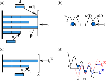
Figure 1: Biased random walk model for filaments and motors:(a) Multiple ($N>1$) filaments against a wall (see lacostenjp2011 for a detailed study of this model). Polymerization and depolymerization rates are $u$ and $w$, when the filaments are away from wall (hence force-free). Note that, when more than one filament touches the wall simultaneously, the depolymerization rate becomes independent of the force(${w}$), as a single depolymerization event cannot cause any wall movement. (b) Multiple motors moving on a track. Note that only the leading motor bears the force $f$, while the trailing motors are experiencing force through hard core interaction. (c) Two filaments at the collective stall force $f_{s}^{(2)}$ undergoing simple processes of polymerization and depolymerization. (d) Two motors diffusing on a tilted free-energy landscape. The force is acting only on the leading motor, and the energy landscape of the leading motor changes with the application of force. Due to hard-core interaction, a larger force($>f_{s}^{(1)}$) is required to stall the system of two motors. It is like moving uphill, with the assistance of a trailing motor, which rectifies the average backward motion of the leader Astumian917 .

Based on these arguments, if one assumes that the system is in equilibrium at stall, the tools of equilibrium statistical mechanics can be applied to calculate the stall forces. Here we show that the stall forces are additive for multiple filaments in the simplest model, where only polymerization and depolymerization processes are involved (see Fig.1(c)). We first consider the dynamics of a single filament under the stall force $f=f_{s}^{(1)}$ applied via the right wall. Let the wall position be $x$ in terms of the subunit size (see Fig.1(c)). Using equilibrium statistical mechanics we can write the probability distribution of the wall-position $P(x)$ as below

$$P(x)=\frac{1}{Z}e^{-\beta f_{s}^{(1)}x}e^{\beta\epsilon x}=\frac{1}{Z}e^{-\beta(f_{s}^{(1)}-\epsilon)x},$$ (1)

where $Z$ is the partition function, and $\epsilon=\ln(u/w)$ is the free energy gained per subunit through polymerization. Note that the term $e^{-\beta f_{s}^{(1)}x}$ appears as we have a Gibbs ensemble in $1$-dimension with fixed external compressive force ($f_{s}^{(1)}$). However, this distribution $P(x)$ should be independent of $x$, as the stall condition can be reached at any position $x$. As per Eq. 1, this implies that $f_{s}^{(1)}=\epsilon=\ln(u/w)$. This same expression has been obtained in earlier theories from a detailed kinetic calculation lacostenjp2011 . Next, we consider a two-filament system subjected to their stall force $f_{s}^{(2)}$ as shown in Fig.1(c). Let the tip-position of the trailing filament be $x_{1}$, which is between $0$ and the wall position $x$. The probability distribution of the wall-position, if the system is in thermodynamic equilibrium, is:

$$P(x)=\frac{1}{Z}e^{-\beta f_{s}^{(2)}x}e^{\beta\epsilon x}(2\sum_{x_{1}=0}^{x}e^{\beta\epsilon x_{1}}-e^{\beta\epsilon x})$$

$$\sim e^{-\beta(f_{s}^{(2)}-2\epsilon)x},\leavevmode\nobreak\ \leavevmode\nobreak\ \leavevmode\nobreak\ \mbox{for large}\leavevmode\nobreak\ \leavevmode\nobreak\ x$$ (2)

A factor of $2$ appears on the right hand side, since there could be two equally likely situations – either the top-filament or the bottom-filament can be the leader (see Fig. 1(c)). Again, $P(x)$ is expected to be independent of $x$, implying that $f_{s}^{(2)}=2\epsilon=2f_{s}^{(1)}$. This argument can be easily extended to $N>2$, and thus $f_{s}^{(N)}=Nf_{s}^{(1)}$ for this simple model. Some arguments, based on detailed balance criterion, have also been given in Refs. doorn2000 and krawczykepl2011 to show similar result of $f_{s}^{(N)}\propto N$ for their respective models on cytoskeletal filaments. However, we demonstrate that a simple calculation based on elementary statistical mechanics, for essentially kinetic processes, leads to the same conclusion.

We now develop similar arguments to show the additivity of stall forces for multiple motors. The forward and backward hopping processes for motors can be viewed as random walks on a tilted free-energy landscape (see Fig.1(d)). In this case, $x$ and $x_{1}$ should be interpreted as the positions of the leading and the trailing motors respectively, for a two-motor system. The free energy ‘released’ per unit step by going downhill on the free-energy landscape is $\epsilon$ (equivalent to the polymerization energy). For a single motor under stall force, we can write the same equation as before (Eq. 1) for the probability distribution of the leading motor’s position, $P(x)$, by recognizing the system to be in equilibrium at stall. However, for two motors at stall, the probability distribution of the leader’s position is somewhat different from the previous case of the filaments, since motors cannot overtake each other. The distribution of the leader’s position is

$$P(x) = \frac{1}{Z}e^{-\beta f_{s}^{(2)}x}e^{\beta\epsilon x}(\sum_{x_{1}=0}^{x-1}e^{\beta\epsilon x_{1}})$$ (3)

$$\sim e^{-\beta(f_{s}^{(2)}-2\epsilon)x},\leavevmode\nobreak\ \mbox{for large}\leavevmode\nobreak\ x.$$

Again, using the argument that $P(x)$ should be independent of $x$, we get back the force additivity : $f_{s}^{(2)}=2\epsilon=2f_{s}^{(1)}$.

In summary, we show that the stall forces are additive for the simple models considered here. This demonstration hinges on the recognition that the systems are in equilibrium at stall, which may not be true in many biological situations. In fact, we show in the next sections that there are many classes of models for which the equilibrium description is simply not feasible, and consequently more complex models have interesting implications.

III Stall forces are non-additive for biologically relevant non-equilibrium models

In this section, we present several case studies to show that the force inequality ($f_{s}^{(N)}\neq Nf_{s}^{(1)}$) is true in general for stall dynamics departing from equilibrium – however, for certain combinations of kinetic rates the relationship $f_{s}^{(N)}=Nf_{s}^{(1)}$ can be retrieved. We begin by analyzing various models of cytoskeletal filaments.

III.1 A random hydrolysis model for cytoskeletal filaments

In cytoskeletal filaments (such as, microtubules and actin filaments), subunits are typically bound to ATP/GTP molecules. When the subunits are connected to the filaments, the ATP/GTP molecules release phosphate and convert to ADP/GDP in a process known as ATP/GTP hydrolysis howardbook ; Alberts2002 . The ADP/GDP-bound monomers have much higher depolymerization rates compared to ATP/GTP-bond monomers Pollard1986 ; Desai_Mitchison_MT:97 . Due to this heterogeneity the cytoskeletal filaments exhibit interesting properties such as ‘dynamic instability’ PhysRevLett.70.1347 . The dynamics of the cytoskeletal filaments have been theoretically studied by many researchers using the “random hydrolysis” model vavylonis:05 ; Ranjith2010 ; Ranjith2012 ; sumedha ; Antal-etal-PRE:07 . Here, we focus on the simplified model of this process as discussed in Refs. dd2014 ; Ranjith2012 , where we neglect complexities related to biofilaments such as structural details, mechanical flexibility, possible interplay between mechanical forces and hydrolysis events and the possible multi-stage nature of the hydrolysis process howardbook ; Desai_Mitchison_MT:97 ; Korn638 ; vavylonis:05 ; 10.1371/journal.pbio.1001161 . As shown in Fig. 2(a), we consider multiple filaments undergoing random hydrolysis and growing against a wall held by a constant opposing force $f$. In the model, each monomer can be in two states: T (ATP/GTP-bound), and D (ADP/GDP-bound). Only T monomers bind to the filaments with a rate $u(f)=u{\rm e}^{f}$ (next to the wall) or $u$ (away from the wall). The rate $u$ is proportional to the concentration ($c$) of T monomers and is defined as $u=k_{0}c$. The depolymerization occurs with a rate $w_{T}$ if the tip-monomer is T, and $w_{D}$ if it is D. For simplicity we assume that there is no force dependence on the off-rates $w_{T}$ and $w_{D}$ (i.e., $\delta=1$). Hydrolysis (T to D conversion) happens randomly on any T subunit in space with a rate $r$. Note that the conversion T$\rightarrow$D is irreversible, as it is not balanced by a reverse conversion, which makes the dynamics inherently non-equilibrium. The exact analytical result for the stall force $f_{s}^{(N)}$ is not known for such a detailed model. Instead we numerically simulate the model using the Gillespie algorithm Gillespiejpc1977 (see Appendix A) with experimentally known rates howardbook ; Pollard1986 ; Desai_Mitchison_MT:97 for microtubules and actin filaments.

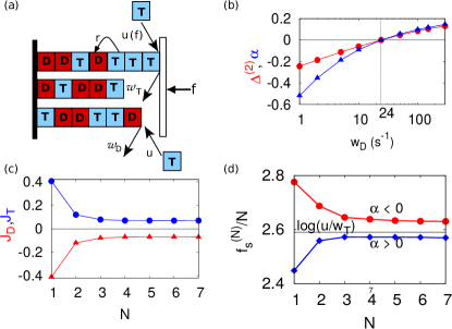
Figure 2: Random hydrolysis model with three filaments, where individual monomer switches from T to D unidirectionally and randomly. Different processes are shown by arrows. $k_{0}=3.2\leavevmode\nobreak\ \mu{\rm M}^{-1}s^{-1}$, $c=100\mu$M, $w_{T}=24s^{-1}$, and $r=0.2s^{-1}$. (a) $\Delta^{(2)}$ (red curve) and $\alpha$ (blue curve) versus $w_{D}$. Note that both $\alpha$ and $\Delta^{(2)}$ are zero only at $w_{T}=w_{D}$ and they are highly correlated in sign. (b) The fluxes per filament (defined in the text), at stall, for T and D monomers as a function of the filament number $N$ for $w_{D}=290s^{-1}\leavevmode\nobreak\ (\alpha>0)$. (c) The collective stall force per filament ($f_{s}^{(N)}/N$) against $N$, the number of filaments. For $\alpha>0$, $w_{D}=290s^{-1}$ and for $\alpha<0$ , $w_{D}=5s^{-1}$

Before proceeding to discuss the issue of stall force additivity, we define a parameter, the “force deviation”:

$$\Delta^{(N)} = f_{s}^{(N)}-N\leavevmode\nobreak\ f_{s}^{(1)}$$ (4)

This parameter represents the excess/deficit of the collective stall force generated by $N$ filaments, as compared to $N$ times the force generated by a single filament. So the deviation $\Delta^{(N)}\neq 0$ implies the violation of force equality, $f_{s}^{(N)}=Nf_{s}^{(1)}$.

As noted before, the random hydrolysis model is a non-equilibrium model by construction. To understand the implications of this non-equilibrium nature, we first look at the energetics associated with the polymerization/depolymerization processes. A growing filament clearly performs work against an applied load $f$ through polymerization. The work done for addition of one subunit to the filament is simply $fd$, where we can take subunit-size $d=1$ without losing any generality. At the stall force $f=f_{s}^{(1)}$, the filament delivers the maximum work $W_{\rm poly}^{\rm max}=f_{s}^{(1)}$. The free energy input to the filament in order to do this work is provided by polymerisation and can be written as $F_{\rm poly}=\ln(u/w_{T})$, per subunit addition. Note that D monomers do not polymerize, and hence there is no contribution in $F_{\rm poly}$ due to D monomers. Finally we define the following quantity for a single filament

$$\alpha=F_{\rm poly}-W_{\rm poly}^{\rm max}=\ln(u/w_{T})-f_{s}^{(1)}$$ (5)

The quantity $\alpha$ signifies how different the maximum work produced per filament is, as compared to the free energy input. Hence, $\alpha$ is analogous to the thermodynamic efficiency of the system niraj:prl-efficiency .

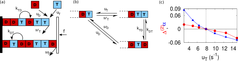
Figure 3: (a) Schematic diagram of a generalized random hydrolysis model with two-way switching (both T$\rightarrow$D, and D$\rightarrow$T). Different processes (shown in arrows) are discussed in the text. (b) Schematic depiction of a connected loop in the configuration space of a single filament, within the model. (c) Deviation ${\Delta}^{(2)}$ versus $u_{T}$ (the red curve), and $\alpha$ versus $u_{T}$ (the blue curve), for the generalized random hydrolysis model. The parameters are: $w_{T}=2s^{-1},k_{TD}=0.3s^{-1},k_{DT}=0.4s^{-1},u_{D}=3s^{-1}$, and $w_{D}=1s^{-1}$.

In Fig.2(b) we plot the deviation $\Delta^{(2)}$ and the efficiency $\alpha$ for two microtubules, against the dissociation rate $w_{D}$ of D monomers. Interestingly, $\Delta^{(2)}$ and $\alpha$ are correlated in the numerical sign. This gives us a hint that the violation of force additivity has something to do with the imbalance between the work produced and the free-energy input (i.e., the departure from equilibrium). To appreciate this interconnection between $\Delta^{(2)}$ and $\alpha$, we proceed to investigate the particle fluxes of the T and D monomers.

We calculate the particle fluxes when the $N$-filament system is at stall. In the simulations Gillespiejpc1977 we separately keep track of the numbers of T and D monomers binding (or unbinding) at a filament-tip in a $N$-filament system. The fluxes are then calculated over a time window. The flux for T monomers per filament ($J_{T}$) is defined as the net change of T monomer numbers at any one filament-tip, divided by the size of the time window. Similarly, we also calculate the flux per filament for D monomers ($J_{D}$). In Fig. 2(c), we show these fluxes at stall. Although we have $J_{T}+J_{D}=0$ (which is expected at stall), individually the fluxes per filament (both $J_{T}$ and $J_{D}$) are non-zero signifying the non-equilibrium nature of the dynamics. An important point to note is that, the fluxes per filament, at stall, decrease with the number of filaments, $N$, and tend to saturate. From this observation, we are tempted to make a hypothesis that a non-equilibrium system with a large number of filaments is closer to “equilibrium” in comparison to a single-filament system(see Appendix B for a crude entropy production argument for this hypothesis).

With this hypothesis in hand, we now attempt to explain why the numerical signs of $\Delta^{(2)}$ and $\alpha$ are correlated (Fig. 2(b)). We first consider the case $\alpha>0$, when a single filament performs less work than the free-energy provided by the polymerization (see Eq. 5). In this case, some energy is dissipated by the filament due to the internal T$\rightarrow$D transitions. As per our hypothesis, if the two-filament system is closer to equilibrium as compared to a single filament, the two-filament system should extract more work by increasing the stall force per filament. To check this, in Fig.2(d), we show the stall force per filament (i.e., the maximum work extracted per filament), $f_{s}^{(N)}/N$ as a function of the filament number $N$. The stall force per filament indeed increases with $N$ for $\alpha>0$, and saturates near the net free-energy input ($\ln(u/w_{T})$). In other words, as the number of filaments increases, the collective stall force per filament gets closer to the “equilibrium” value of $\ln(u/w_{T})$. This increase in stall force per filament makes $f_{s}^{(2)}/2>f_{s}^{(1)}$ and in return gives positive $\Delta^{(2)}$. Thus, the $\alpha>0$ case correlates with $\Delta^{(2)}>0$. Similar arguments can be given for $\alpha<0$ (see Fig.2(d)), where a single filament performs more work than the energy provided by polymerization. To bring the system closer to equilibrium, the two-filament system decreases the stall force per filament ($f_{s}^{(N)}/N<f_{s}^{(1)}$). Hence, $\Delta^{(2)}$ is negative if $\alpha<0$.

An interesting point to note in Fig.2(b) is that both $\Delta^{(2)}$ and $\alpha$ are zero exactly at $w_{T}=w_{D}$. This shows that T$\rightarrow$D switching (hydrolysis) is necessary to produce the phenomenon of non-additivity of stall forces. It is to be noted that the hydrolysis is always a non-equilibrium process as it is unidirectional. However, the condition $w_{T}=w_{D}$ effectively corresponds to absence of switching, since dynamically there remains no distinction between T and D subunits. The filaments cannot “sense” their distinct presence as far as the force generation is concerned. Yet, the condition $w_{T}=w_{D}$ does not imply a true equilibrium until we set the T$\rightarrow$D switching rate to zero. Another way to possibly achieve equilibrium at stall is to incorporate the reverse switching (D$\rightarrow$T) and allow the polymerization of D subunits. Although these additions are biologically unrealistic, we nevertheless study such a model in the next section to explore the relevance of non-equilibrium dynamics for non-additivity of the stall forces.

III.2 A generalized random hydrolysis model for filaments

We make the random hydrolysis model (discussed in section III.1) more general and symmetric by allowing (i) D $\to$ T conversion, and (ii) addition of both D and T monomers to the filaments. In this model (see Fig.3(a)) both T and D subunits can bind to a filament with constant rates $u_{T}$ and $u_{D}$, respectively. When the filaments come in contact with the wall (see Fig.3(a)), the polymerization rates decrease to $u_{T}(f)=u_{T}\rm{e}^{-f}$ and $u_{D}(f)=u_{D}\rm{e}^{-f}$ in the presence of the force $f$ (using the load distribution factor $\delta=1$ for simplicity). The depolymerization occurs with a rate $w_{T}$ if the tip-monomer is T, or $w_{D}$ if it is D. Any randomly chosen subunit inside a filament can convert either from T to D (with rate $k_{TD}$), or from D to T (with rate $k_{DT}$).

Within the general version of the random hydrolysis model, we now proceed to show that the two-way switching (T $\to$ D, and D $\to$ T) in general produces non-equilibrium dynamics that is embodied in the violation of the condition of detailed balance for the kinetic rates. For a single filament, as shown in Fig. 3(b), we consider a loop of dynamically connected configurations. The product of clockwise and anticlockwise rates are $u_{T}k_{TD}w_{D}$ and $u_{D}k_{DT}w_{T}$, respectively. For the condition of detailed balance, that is, equilibrium, to be reached at steady state, the two products must be equal according to the Kolmogorov’s criterion  kolmogorov1936 ; book-kolmogorov (or the Wegschieder condition Wegsch ), which leads to

$$\frac{u_{T}}{w_{T}}\frac{k_{TD}}{k_{DT}}\frac{w_{D}}{u_{D}}=1.$$ (6)

If we fix the parameters $w_{T}=2s^{-1},k_{TD}=0.3s^{-1},k_{DT}=0.4s^{-1},u_{D}=3s^{-1}$, and $w_{D}=1s^{-1}$, then we would have $u_{T}=8s^{-1}$ from the above equilibrium condition (Eq. 6). Though this criterion is written in terms of force-free rates, it is clear that using the modified rates in the presence of the resisting force would not change the condition in Eq. 6. We now plot the deviation $\Delta^{(2)}=f_{s}^{(2)}-2f_{s}^{(1)}$ versus $u_{T}$ in Fig.3(c) – see the red curve (data from stochastic simulation). The plot quite interestingly shows that $\Delta^{(2)}=0$ only at $u_{T}=8s^{-1}$; otherwise it is nonzero. This clearly indicates that the phenomenon of non-additivity of stall forces is tied to the departure of the system from equilibrium. This can be compared with the arguments given in section II, where it is shown that the filament models involving no switching exhibit equilibrium at stall, and consequently the relationship $f_{s}^{(N)}=Nf_{s}^{(1)}$ holds without any restriction.

We can further relate the non-equilibrium effect of non-additivity of the force with the imbalance between the free energy input and maximum work output (as discussed in section III.1). Because, in the present model, the filaments can grow by adding D or T monomers, the free energy input to the system should depend on polymerization energies corresponding to both T and D monomers. Consequently, the partition function for a single filament is $e^{\epsilon_{T}}+e^{\epsilon_{D}}$ (using $k_{B}T=1$), where $\epsilon_{T}$ and $\epsilon_{D}$ are polymerization energies provided by T and D monomers, respectively. Hence, the free energy input to the filament is $F_{\rm poly}=\ln[e^{\epsilon_{T}}+e^{\epsilon_{T}}]=\ln[(u_{T}/w_{T})+(u_{D}/w_{D})]$; and the maximum work done by the filament is simply $f_{s}^{(1)}$ (using subunit size $d=1$). Following previous section III.1, we again define an efficiency-like parameter for the current model as below

$$\alpha=F_{\rm poly}-W_{\rm poly}^{\rm max}=\ln[(u_{T}/w_{T})+(u_{D}/w_{D})]-f_{s}^{(1)}$$ (7)

We see in Fig.3(c) that both $\alpha$ and $\Delta^{(2)}$ are correlated in numerical sign, and they are non-zero every where except for a single point where the system is in equilibrium at stall (according to Eq. 6). With this understanding of the connection between the non-equilibrium dynamics and non-additivity of stall forces, we study another model for filaments dd2014 in the next section, and show that the same ideas can be carried forward.

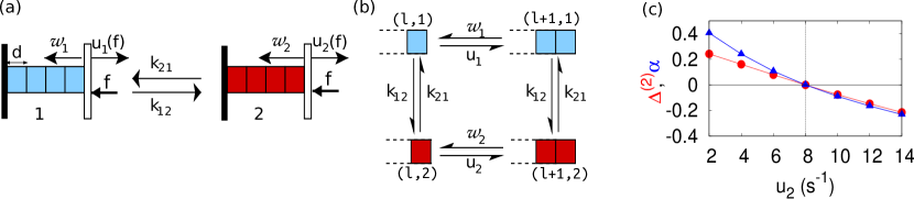
Figure 4: (a) Schematic diagram of single-filament 2-state model with switching between states $1$ (blue) and $2$ (red). Various processes are shown by arrows and corresponding rates, as discussed in the text. (b) Schematic depiction of a connected loop in the configuration space of single-filament 2-state model. The configurations are denoted by ordered pairs, whose first element is the instantaneous length and second element is the chemical state ($1$ or $2$). (c)$\Delta^{(2)}$ (red) and $\alpha$ (blue) as a function of $u_{2}$ for the 2-state model. Parameters are $k_{12}=0.5\leavevmode\nobreak\ s^{-1}$, $k_{21}=0.5\leavevmode\nobreak\ s^{-1}$, $w_{1}=0.1\leavevmode\nobreak\ s^{-1}$ $u_{1}=1\leavevmode\nobreak\ s^{-1}$, $w_{2}=0.8\leavevmode\nobreak\ s^{-1}$.

III.3 A two-state model for filaments

In the literature dd2014 ; hill:84-2 , there exists a model which incorporates the detailed process of hydrolysis in a more coarse-grained way. In this model (Fig.4(a)), each filament can switch between two chemical states $1$ and $2$, with switching rates $k_{12}$ (from $1$ to $2$), and $k_{21}$ (from $2$ to $1$). In the states $1$ and $2$, the filament has distinct depolymerization rates $w_{1}$ and $w_{2}$, respectively, and polymerization rates of $u_{1}$ and $u_{2}$, respectively (see Fig.4(a)).If a filament bears the load (i.e., touches the wall), its polymerization rate is modified to $u_{i}(f)=u_{i}{\rm e}^{-f}$ $(i=1,2)$. For simplicity, we assume that the depolymerization rates are force independent.

For the above two-state model, we first explicitly show that at stall the dynamics is non-equilibrium. As shown in Fig.4(b), we consider a loop of connected configurations for a single filament characterized by its length and state. In this case, Kolmogorov’s criterion reduces to

$$u_{1}k_{12}w_{2}k_{21}=k_{12}u_{2}k_{21}w_{1}$$

$$\Longrightarrow\frac{u_{1}}{{w}_{1}}=\frac{u_{2}}{{w}_{2}}$$ (8)

Following the procedure involving microscopic master equations, as described in Ref. dd2014 , we analytically obtain the single-filament and two-filament stall forces ($f_{s}^{(1)}$, $f_{s}^{(2)}$) In Fig.4(c), we plot $\Delta^{(2)}$ against $u_{2}$ (red curve) with fixed $w_{1}=0.1s^{-1}$, $u_{1}=1s^{-1}$, and $w_{2}=0.8s^{-1}$. We find that ${\Delta}^{(2)}\neq 0$ for all $u_{2}$, except for $u_{2}=8s^{-1}$ (the value corresponding to the equality in Eq. 8). This shows that the non-additivity of stall forces is tied to the departure from equilibrium.

It is to be noted that in the two-state model , $\ln(u_{i}/{w}_{i})$ is the polymerization free energy in state $i=(1,2)$. Hence, if $P_{i}$ is the probability of finding a filament in a state $i$, then at any instant the amount of free energy that is transferred from the bath of monomers to the filament by addition of monomers of type $1$ or $2$ is $F_{\rm poly}=P_{1}\ln(u_{1}/{w}_{1})+P_{2}\ln(u_{2}/{w}_{2})$. On the other hand, the maximum amount of work done by a filament against the applied force is $W^{\rm max}=f_{s}^{(1)}$ (monomer size being $d=1$). Therefore, as defined in the previous sections, we can again define an efficiency parameter as:

$$\alpha=F_{\rm poly}-W^{\rm max}=[P_{1}\ln(u_{1}/{w}_{1})+P_{2}\ln(u_{2}/{w}_{2})]-f_{s}^{(1)},$$ (9)

where, $P_{1}=k_{21}/(k_{12}+k_{21})$ and $P_{2}=k_{12}/(k_{12}+k_{21})$. These probabilities follow from the fact that the detailed balance relation $P_{1}k_{12}=P_{2}k_{21}$ holds at the steady state for a single filament, as intuitively evident from the Fig.4(a) (also see Ref dd2014 ), along with the normalization condition $P_{1}+P_{2}=1$. In Fig.4(c), we plot $\alpha$ versus $u_{2}$ (blue curve). We see that $\Delta^{(2)}$ is closely coupled to $\alpha$ in numerical sign, and both are nonzero except at the point where the equilibrium condition (Eq. 8) is satisfied.

The effect of non-additivity of stall forces is not specific to cytoskeletal filaments. Even the system of multiple molecular motors show such a behavior joanny2006prl ; casademunt2015nature . In the ensuing sections, we explore the connection between the non-additivity of the force with the non-equilibrium dynamics in the system of motors.

III.4 Model of interacting motors by Campàs et al.

A model of multiple interacting motors pushing against a load has been recently proposed by Campàs et al. joanny2006prl . In this model (Fig. 5a), motors walk along a one-dimensional lattice (lattice spacing $d=1$) and move by a single step forward (rate $u$) or backward (rate $w$). There is hard core interaction between the motors. The leading motor alone bears the load, and hence its hopping rates are modified to $u(f)=u{\rm e^{-f\delta}}$, and $w(f)=w{\rm e^{f(1-\delta)}}$, where $\delta$ is the force distribution factor. The hopping rates also change due to nearest-neighbour interactions – if a motor is adjacent to another one, its forward and backward hopping rates become $\bar{u}$ and $\bar{w}$, respectively (see Fig. 5(a)).

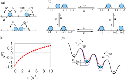
Figure 5: (a) Schematic diagram of the motor model proposed by Campàs et al. joanny2006prl , where multiple interacting motors push against a cargo with a constant force $f$ acting against their motion. Various processes are shown by arrows and discussed in the text. (b) Schematic depiction of a closed loop of dynamically connected configurations for the model shown in (a). (c)Deviation ${\Delta}^{(2)}$ versus $\bar{u}$ within the model of Campàs et al (data obtained from the exact formula given in joanny2006prl ). Parameters are specified in the text. We took the force distribution factor $\delta=1$.(d)Motors walking on a free-energy landscape joanny2006prl . The effect of nearest-neighbour interactions is shown schematically.

From analytical calculations and numerical simulations, the authors have found that the stall forces are not necessarily additive. We show here that the non-additivity is a manifestation of the non-equilibrium nature of the dynamics. To show this we apply the Kolmogorov criterion, by making a closed loop of connected configurations as shown in Fig.5(b). By equating the clockwise and counter-clockwise products of rates along the loop, we have

$$u.\bar{u}.w.w=\bar{w}.u.u.w$$

$$\Longrightarrow\frac{u}{w}=\frac{\bar{u}}{\bar{w}}$$ (10)

Exact analytical expressions of the single-motor stall force $f_{s}^{(1)}={\rm ln}(u/w)$, and the two-motor stall force $f_{s}^{(2)}={\rm ln}[(u\bar{u}/w\bar{w})+(u/w)-(\bar{u}/\bar{w})]$ are derived in Ref joanny2006prl . If we put the equality of Eq. 10 in the expression of $f_{s}^{(2)}$, we clearly see that the relationship $f_{s}^{(2)}=2f_{s}^{(1)}$ follows. We further plot (Fig. 5(c)) $\Delta^{(2)}=f_{s}^{(2)}-2f_{s}^{(1)}$ versus $\bar{u}$, with fixed $u=20s^{-1}$,$w=5s^{-1}$, and $\bar{w}=1s^{-1}$. In this case, $\bar{u}=4s^{-1}$ corresponds to equilibrium dynamics (Eq. 10), and we see that except for $\bar{u}=4s^{-1}$, $\Delta^{(2)}\neq 0$ everywhere. This corroborates our hypothesis that the additivity of stall forces is closely linked with the underlying equilibrium of the system, a point not recognized in Ref. joanny2006prl .

We can also obtain the condition of equilibrium (Eq. 10) from a simple thermodynamic argument by considering the hopping processes of the motors on a free-energy landscape (see Fig. 5(d)). Due to the nearest-neighbour interactions, the shape of the free energy landscape gets altered when the motors are adjacent to each other. An attractive interaction deepens the energy wells by an amount $e_{\rm int}$ (dotted blue curve in Fig. 5(d)), and makes it hard for the particles to leave the position. This reduces the forward and backward hopping rates. On the other hand, the repulsive interaction makes the potential wells shallower (dotted red curve in Fig. 5(d)), which makes it easy for the particles to hop forward or backward. In this case, hopping rates increase from the original values. When the motors are adjacent to each other, following Fig. 5(d), the hopping rates are given by

$$\frac{u}{\bar{w}} = e^{\epsilon-e_{\rm int}}$$ (11)

$$\frac{\bar{u}}{w} = e^{\epsilon+e_{\rm int}}$$ (12)

For a motor which is away from the other one, $e_{\rm int}=0$, and we further have

$$\frac{u}{w}=e^{\epsilon}$$ (13)

By rearranging the equations 11, 12 and 13, we get back the same condition, $\frac{u}{w}=\frac{\bar{u}}{\bar{w}}$, as in Eq. 10, which is a reflection of the equilibrium dynamics at stall.

III.5 A motor model with multiple step-sizes

It was found tripti2013 ; roopmallik2004 recently that dynein motors on a microtubule can take multiple step sizes – predominantly $24$-nm and $32$-nm steps. This inspired us to cast a new model of motors walking with two distinct step sizes (see Fig. 6(a)). A motor at a lattice site $i$ can hop to any of the sites $i+1$ (with rate $u_{1}$), $i+2$ (with rate $u_{2}$), $i-1$ (with rate $w_{1}$), or $i-2$ (with rate $w_{2}$). The leading motor alone bears the applied force $f$ and its forward rates are modified to $u_{1}(f)=u_{1}{\rm e^{-f}}$ and $u_{2}(f)=u_{2}{\rm e^{-2f}}$, while the backward rates are assumed to be force-independent. Unlike the model in the previous section (Section III.4) there is no explicit attractive or repulsive interaction between the motors.

Proceeding in a similar way as described in section III.2, we first derive the condition for equilibrium, by considering a closed loop of connected configurations as shown in Fig. 6(b). Following Kolmogorov criterion we get

$$u_{1}^{2}.w_{2}=u_{2}.w_{1}^{2}$$

$$\Longrightarrow\frac{u_{2}}{w_{2}}=\left(\frac{u_{1}}{w_{1}}\right)^{2}$$ (14)

If we take $u_{1}=80s^{-1},w_{1}=8s^{-1}$, and $w_{2}=1s^{-1}$, then $u_{2}=100s^{-1}$ is the value corresponding to the equilibrium condition (see Eq. 14). In Fig. 6(c), $\Delta^{(2)}$ versus $u_{2}$ is plotted from our simulation results (the red curve), where we see that indeed $\Delta^{(2)}=0$ only for $u_{2}=100s^{-1}$. Thus, one can again associate the force inequality $f_{s}^{(N)}\neq Nf_{s}^{(1)}$ to the violation of the detailed balance condition.

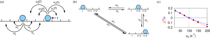
Figure 6: Multiple step size motor model: (a) Schematic diagram of the motors moving with two distinct step sizes. The kinetic processes (shown in arrows) are explained in the text. (b) A closed loop of connected configurations for the model with one motor. (c) Deviation ${\Delta}^{(2)}$ versus $u_{2}$ (the red curve), and $\alpha$ versus $u_{2}$ (the blue curve). The parameters are $u_{1}=80s^{-1},w_{1}=8s^{-1}$, and $w_{2}=1s^{-1}$.

Just like the models of filaments discussed in the previous sections (Sections III.1, III.2 and III.3), we can show that the effect of force-additivity for motors is related to the underlying energetic imbalance. The motor model with multiple step-sizes looks conceptually similar to the generalized random hydrolysis model (see Section III.2). At any instant, a filament can grow by adding T or D monomers in the generalized random hydrolysis model; whereas in the current model a motor can move forward (or backward) by taking steps of sizes $d$ or $2d$. These steps of size $d$ and $2d$ involve different amounts of work done by a single motor at stall ($f_{s}^{(1)}d$ and $f_{s}^{(1)}2d$ respectively). By contrast, addition of a D or T monomer to a single filament leads to the extraction of the same amount of work ($f_{s}^{(1)}d$). Hence, for the definition of the efficiency parameter, $\alpha$, we choose to take into account the energy imbalance that results from a single step of size $d$. For a single motor taking a step of unit lattice size, we can write the free-energy supplied by ATP molecules as $F=\ln(u_{1}/w_{1})$ and the maximum work done as $W^{\rm max}=f_{s}^{(1)}$ (considering the lattice spacing $d=1$). Thus, we can define an efficiency-like quantity as

$$\alpha=F-W^{\rm max}=\ln(u_{1}/w_{1})-f_{s}^{(1)}.$$ (15)

We do not claim that this is a unique definition of $\alpha$ for the system. One may certainly come up with some other definition of $\alpha$, for example,

$$\alpha={1\over 2}(\ln{u_{2}\over w_{2}}-2f_{s}^{(1)}),$$ (16)

to quantify the excess/deficit of energy supply to the system. Note that both the definitions of $\alpha$ (Eqs. 15 and 16) essentially capture the energy imbalance per unit step.

We plot $\alpha$ (from Eq. 15) and $\Delta^{(2)}$ versus $u_{2}$ in Fig.6(c), and see that both $\alpha$ and $\Delta^{(2)}$ are indeed correlated in numerical sign. Moreover, both of them are zero only when the equilibrium condition (Eq. 14) is satisfied. The same finding can be derived using the other definition of $\alpha$, that is, using Eq. 16 instead of Eq. 15 (data not shown). This further strengthens our point that non-additivity of stall forces is a manifestation of underlying non-equilibrium stall dynamics.

IV Discussion and conclusion

Collective force generation by filaments or motors has been theoretically studied by many researchers using various models in specific contexts doorn2000 ; lacostenjp2011 ; Kierfeld:2013 ; dd2014 ; joanny2006prl ; CasademuntPRL2009 ; kolomeiskyjcp2004 ; dd2014-2 ; Ambarish2010phybio ; Bouzat2010phybio ; PhysRevE.91.022701 . However, a broad picture explaining the cooperative effects in stall (maximum) force generation is still missing. In this paper we have provided a theoretical framework to understand and predict the cooperative effects in the maximum force generation by multiple motors or filaments, for a broad class of models. It is now appreciated, at least theoretically, that the stall force of individual cytoskeletal filaments or molecular motors, when they push together against some obstacle, is not additive in general dd2014 ; joanny2006prl ; kolomeisky2015 . In this paper, we have provided several pointers to show that this non-additivity of the stall forces ($f_{s}^{(N)}\neq Nf_{s}^{(1)}$) is a manifestation of the underlying non-equilibrium nature of the dynamics at stall.

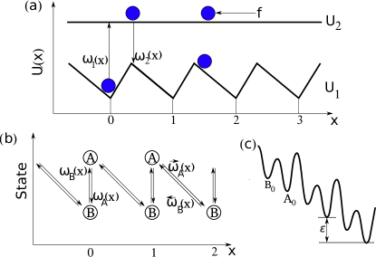
Figure 7: Schematic of the (a) continuous julicher1997 and (b) discrete two-state Brownian ratchet model lacoste2007 ; lacoste2008 . (a) A spontaneous motion is expected when the ratio of transition rates $\omega_{1}(x)\over\omega_{2}(x)$ is far from the equilibrium value given by the detailed balance condition.(b) Discrete version of the two-state ratchet model with effective transition rates $\overrightarrow{\omega}_{A}(x)$, $\omega_{A}(x)$, $\omega_{B}(x)$ and $\overleftarrow{\omega}_{B}(x)$.(c)Energy landscape corresponding to discrete two-state model.

Our study suggests that if the Kolmogrov criterion for kinetic rates is satisfied then one does not need a detailed non-equilibrium calculation to obtain the stall force of multiple filaments/motors. The same result can be obtained from a simple equilibrium statistical mechanics calculation. Moreover, even if the Kolmogrov criterion for kinetic rates is not satisfied for a system, our efficiency parameter $\alpha$ qualitatively predicts that the cooperative effects in the stall force for multiple filaments (or motors) is either enhanced or decreased as one increases the number of filaments (or motors). For a class of models discussed in this paper, we clearly see a correlation between the numerical signs of $\alpha$ and the force deviation $\Delta^{(2)}$. We would like to point out that the Kolmogorov or Wegschieder criterion for detailed balance has been used earlier in the context of multiple growing filaments  krawczykepl2011 to describe the linear scaling of the stall force with the number of filaments. We, however, used the Kolmogorov criterion to systematically probe a range of models and derive the conditions that must be obeyed by their respective kinetic rates, if the systems are expected to be in “equilibrium” at stall. More importantly, the conceptual advantage gained by couching this problem in the language of thermodynamic equilibrium is that, if any similar system is not in equilibrium at stall, then it is not at all guaranteed that the stall forces will be additive with the system size (number); in fact, non-additivity is the more likely outcome.

To illustrate the above point further, we take a concrete example of a two-state motor model from the existing literature joanny2006prl ; CasademuntPRL2009 ; oriola2013 ; oriola2014 ; julicher1997 (Fig. 7), which demostrated the stall force non-additivity $f_{s}^{(N)}\neq Nf_{s}^{(1)}$. Our analysis indicates the same conclusion without the need for any detailed simulation or theoretical calculations. We identify that the violation of detailed balance in the transition rates between the states is a requirement for the spontaneous motion in this two-state Brownian ratchet model (see Fig. 7(a)). As a result, even for a single motor at stall, although the mean velocity flux of the motor is zero, the individual velocity fluxes in states-1 and state-2 (with potentials ${\rm U}_{1}$ and ${\rm U}_{2}$, respectively) for the motor are not independently zero. In fact, only by observing the energy landscape one can say that, at stall, the mean particle flux in state-1 and state-2 would be positive and negative, respectively. This is because, the mean particle flux in state-2 is zero in the absence of any resisting force (flat potential, see Fig.7(a)) and would become negative with the application of a resisting force. To make the mean flux of the overall system zero, the effective mean flux in state-1 has to be positive under stall condition. This non-equilibrium at stall for one motor manifests itself in the form of non-additivity of stall forces in the presence of multiple motors even though the only interaction between them is self-exclusion (Fig.7(a)) joanny2006prl ; oriola2013 ; oriola2014 . Interestingly, a discrete version of this two-state model lacoste2007 ; lacoste2008 , shows additivity of stall forces for multiple motors with only self-inclusion interactions (see Fig. 7(b)). This results from the fact that this discrete model for a single motor can easily be mapped to a biased random walk with only one track fisher2001 – the motors effectively move on a tiled energy landscape, $\epsilon=\ln\frac{\omega_{B}\overrightarrow{\omega}_{A}}{\omega_{A}\overleftarrow{\omega}_{B}}$(see Fig. 7), which, as argued in Section II, indicates that the motor can be interpreted to be in equilibrium at stall.

We can generalise the observations noted above and propose that the stall behaviour of passively interacting, processive motors greatly depends on the topology of the mechanochemical migration path of the motors. Consequently, we generally propose that motor models analogous to the ones pioneered by Kolomeisky and Fisher fisher1999 ; fisher2001 with a single track for motor migration will show additivity of stall force for multiple, passively interacting motors. On the other hand, the Brownian models with multiple tracks julicher1997 demonstrably exhibit non-additivity of stall forces for multiple, even passively interacting motors oriola2013 ; oriola2014 . To the best of our knowledge, the general conceptual framework that compares and contrasts the behaviour of these two major classes of molecular motor models, has not been provided before and is also one of the main contributions of this paper.

To summarize, collective force generation in biofilaments and molecular motors typically involve multi-step, complex internal processes and a variety of interactions between the individual entities as well as the source of the resisting force. In this paper we, however, have demonstrated that, even with very simple internal dynamics and also in the absence of any attractive or repulsive interactions between individual components, if a system of molecular motors or filaments is not in equilibrium at stall we can expect non-additivity in their collective force generation. To establish this result with reasonable certainty, we have analyzed, multiple seemingly disparate models, which nevertheless exhibit a common theme of non-equilibrium dynamics at stall leading to this cooperativity. The formalism developed in this paper should provide a general thermodynamics based framework with which to perform primary interpretation of experimental and theoretical results relating to collective force generation in biofilaments and molecular motors, before examining the system related specifics.

Appendix A

Simulation Method

We have simulated our models using kinetic Monte-Carlo algorithm also known as the Gillespie algorithm, BORTZ197510 ; Gillespiejpc1977 ; Gillespiejpc2007 , for the calculation of stall force of analytically unsolvable models . Now we elaborate the exact method we have used to simulate “generalized random hydrolysis model’ for $n=3$ microtubule filaments. We start time evolution of the model system from a fixed initial length of $l_{0}=2000$ monomer at $t=0$ for all the microtubules. To obtain the time at which the next event will occur, we sum all possible event rates, $a_{0}$, and generate a random number $p$ between 0 and 1. Now $\tau\leavevmode\nobreak\ =\leavevmode\nobreak\ \frac{1}{a_{0}}\leavevmode\nobreak\ ln\left(\frac{1}{p}\right)$ is the time of the next event. To determine which event $k$ will occur at time $\tau$, we generate another random number $p_{2}$ between 0 and 1 and find $k$ which satisfies the condition $\sum_{i=1}^{k-1}a_{i}<a_{0}p_{2}\leavevmode\nobreak\ <\leavevmode\nobreak\ \sum_{i=1}^{k}a_{i}$. Now we repeat this processes till our system reaches a steady state. For $n=3$ microtubule, we have taken time to reach steady state as $t=1000s^{-1}$. Now at this point we reset our time to zero and start monitoring the position of largest microtubule filament with time. We plot this time evolution data and from the slope of the plot we get the velocity of the tip of largest filament. We perform this simulation for various forces and obtain corresponding velocity of the barrier. We then draw the force velocity curve. The point at which this force velocity curve cuts the velocity axis is the stall force. To further verify the stall force, we calculate particle flux of the monomers for that force. For the calculation of flux, we just mark one filament and observe the number of monomers being added to that filament$(+1)$ and removed from that filament($-1$). Now we divide this count of monomers by the time window for which this bookkeeping has been done. If this flux is close to zero($>10^{-5}$) then we take that point as the stall force.

Appendix B

Connection between subunit flux and entropy production for multiple biofilaments at stall described using the random hydrolysis model of Section III.1

In the following text, we provide a simple, and perhaps crude, connection between the subunit flux $j_{T}(N)$ per filament, presented in Fig. 2c for the random hydrolysis model of Sec. III.1, and the corresponding coarse grained entropy production $\dot{s}(N)$ per filament for $N$ filament at stall.

Entropy production per filament is given by lacoste2007 ; julicher1997 :

$$\dot{s}=vf+r\Delta\mu,$$ (17)

where $f$, $v$, $\Delta\mu$ and $r$ are the external force, mean velocity, chemical potential for the subunit exchange and subunit exchange flux, respectively. At stall condition, $v=0$, and hence, the entropy production is induced only by subunit exchange flux. For the simple T-D random hydrolysis model described in Sec. III.1, the effective subunit fluxes (per filament) are $j_{T}$ and $j_{D}$, respectively. Moreover, at stall, since the total material influx, on an average, into the system of filaments is zero, $j_{T}=-j_{D}=j$. Since, in this model, the only subunit on rate is $U$ for the T subunits, the chemical potentials corresponding to T and D influx can simplistically be written as

$$\Delta\mu_{T} = \ln{U\over w_{T}},\mbox{ and}$$

$$\Delta\mu_{D} = \ln{U\over w_{D}}.$$ (18)

Using Eqs. 17 and 18, the entropy production at stall condition can now be re-written as

$$\dot{s}(N) = j_{T}(N)\Delta\mu_{T}+j_{D}(N)\Delta\mu_{D}$$ (19)

$$= j(N)\ln{w_{D}\over w_{T}}.$$

Thus, a very simple argument proposes that entropy production per filament at stall condition is proportionate to the subunit flux per filament in the system of multiple filaments.

References

References

- (1) H. Lodish, A. Berk, C. Kaiser, M. Krieger, A. Scott, M.and Bretscher, H. Ploegh, and P. Matsudaira, Molecular Cell Biology, W. H. Freeman New York, NY,USA, 6th edition, 2007.
- (2) P. Nelson, Biological Physics: Energy, Information, Life: With new art by David Goodsell, WH Freeman and Company, 5th edition, 2014.
- (3) B. Alberts, D. Bray, J. Lewis, M. Raff, K. Roberts, and J. Watson, Molecular Biology of the Cell, Garland, 4th edition, 2002.
- (4) N. Hirokawa, S. Niwa, and Y. Tanaka, Neuron 68, 610 (2010).
- (5) R. D. Vale, Cell 112, 467 (2003).
- (6) R. A. Cross and A. McAinsh, Nat Rev Mol Cell Biol 15, 257 (2014).
- (7) C. Bustamante, D. Keller, and G. Oster, Accounts of Chemical Research 34, 412 (2001).
- (8) J. E. Molloy, J. E. Burns, J. Kendrick-Jones, R. T. Tregear, and D. C. S. White, Nature 378, 209 (1995).
- (9) M. Fisher and A. Kolomeisky, Proc. Natl. Acad. Sci. USA. 96, 6597 (1999).
- (10) A. Kolomeisky and M. Fisher, Annu. Rev. Phys. Chem. 58, 675 (2007).
- (11) A. B. Kolomeisky, Journal of physics. Condensed matter : an Institute of Physics journal 25, 10.1088/0953 (2013).
- (12) D. Chowdhury, Physics Reports 529, 1 (2013).
- (13) B. E. Clancy, W. M. Behnke-Parks, J. O. L. Andreasson, S. S. Rosenfeld, and S. M. Block, Nat Struct Mol Biol 18, 1020 (2011).
- (14) T. Bameta, R. Padinhateeri, and M. M. Inamdar, Journal of Statistical Mechanics: Theory and Experiment 2013, P02030 (2013).
- (15) C. Veigel and C. F. Schmidt, Nat Rev Mol Cell Biol 12, 163 (2011).
- (16) P. Ranjith, D. Lacoste, K. Mallick, and J.-F. Joanny, Biophys. J. 96, 2146 (2009).
- (17) A. Desai and T. J. Mitchison, Annu. Rev. Cell. Dev. Biol. 13, 83 (1997).
- (18) A. J. Hunt and J. R. McIntosh, Mol. Biol. Cell 9, 2857 (1998).
- (19) T. L. Hill and Y. Chen, Proc. Natl. Acad. Sci. USA. 81, 5772 (1984).
- (20) M. J. Schnitzer, K. Visscher, and S. M. Block, Nat Cell Biol 2, 718 (2000).
- (21) S. M. Rafelski and J. A. Theriot, Annu. Rev. Biochem. 73, 209 (2004).
- (22) T. E. Schaus and G. G. Borisy, Biophysical Journal 95, 1393 (2008).
- (23) S. L. Kline-Smith and C. E. Walczak, Molecular Cell 15, 317 (2004).
- (24) A. K. Efremov, A. Radhakrishnan, D. S. Tsao, C. S. Bookwalter, K. M. Trybus, and M. R. Diehl, Proceedings of the National Academy of Sciences 111, E334 (2014).
- (25) A. D. Mehta, R. S. Rock, M. Rief, J. A. Spudich, M. S. Mooseker, and R. E. Cheney, Nature 400, 590 (1999).
- (26) G. S. van Doorn, C. Tanase, B. M. Mulder, and M. Dogterom, European Biophysics Journal 29, 2 (2000).
- (27) V. Levi, A. S. Serpinskaya, E. Gratton, and V. Gelfand, Biophysical Journal 90, 318 (2006).
- (28) K. Tsekouras, D. Lacoste, K. Mallick, and J.-F. Joanny, New Journal of Physics 13, 103032 (2011).
- (29) J. Krawczyk and J. Kierfeld, EPL (Europhysics Letters) 93, 28006 (2011).
- (30) B. Zelinski and J. Kierfeld, Phys. Rev. E 87, 012703 (2013).
- (31) D. Das, D. Das, and R. Padinhateeri, New J. Phys. 16, 063032 (2014).
- (32) O. Campàs, Y. Kafri, K. B. Zeldovich, J. Casademunt, and J.-F. Joanny, Phys. Rev. Lett. 97, 038101 (2006).
- (33) J. Brugués and J. Casademunt, Phys. Rev. Lett. 102, 118104 (2009).
- (34) A. Kunwar, M. Vershinin, J. Xu, and S. P. Gross, Curr. Biol. 18, 1173 (2008).
- (35) O. Campàs, C. Leduc, P. Bassereau, J. Casademunt, J.-F. Joanny, and J. Prost, Biophysical Journal 94, 5009 (2008).
- (36) D. D moulin, M.-F. Carlier, J. Bibette, and J. Baudry, Proceedings of the National Academy of Sciences 111, 17845 (2014).
- (37) G. Koster, M. VanDuijn, B. Hofs, and M. Dogterom, Proceedings of the National Academy of Sciences 100, 15583 (2003).
- (38) C. Leduc, O. Camp s, K. B. Zeldovich, A. Roux, P. Jolimaitre, L. Bourel-Bonnet, B. Goud, J.-F. Joanny, P. Bassereau, and J. Prost, Proceedings of the National Academy of Sciences of the United States of America 101, 17096 (2004).
- (39) M. Dogterom and B. Yurke, Science 278, 856 (1997).
- (40) M. E. Janson and M. Dogterom, Phys. Rev. Lett. 92, 248101 (2004).
- (41) D. R. Kovar and T. D. Pollard, Proceedings of the National Academy of Sciences of the United States of America 101, 14725 (2004).
- (42) L. Laan, J. Husson, E. L. Munteanu, J. W. J. Kerssemakers, and M. Dogterom, Proc. Natl. Acad. Sci. USA. 105, 8920 (2008).
- (43) C. Brangbour, O. du Roure, E. Helfer, D. D moulin, A. Mazurier, M. Fermigier, M.-F. Carlier, J. Bibette, and J. Baudry, PLoS Biol 9, 1 (2011).
- (44) J. L. McGrath, N. J. Eungdamrong, C. I. Fisher, F. Peng, L. Mahadevan, T. J. Mitchison, and S. C. Kuo, Current Biology 13, 329 (2003).
- (45) M. E. Janson, M. E. de Dood, and M. Dogterom, The Journal of Cell Biology 161, 1029 (2003).
- (46) Y. Marcy, J. Prost, M.-F. Carlier, and C. Sykes, Proceedings of the National Academy of Sciences of the United States of America 101, 5992 (2004).
- (47) M. Prass, K. Jacobson, A. Mogilner, and M. Radmacher, The Journal of Cell Biology 174, 767 (2006).
- (48) S. H. Parekh, O. Chaudhuri, J. A. Theriot, and D. A. Fletcher, Nat Cell Biol 7, 1219 (2005).
- (49) M. J. Footer, J. W. J. Kerssemakers, J. A. Theriot, and M. Dogterom, Proc. Natl. Acad. Sci. USA. 104, 2181 (2007).
- (50) C. S. Peskin, G. M. Odell, and G. F. Oster, Biophys. J. 65, 316 (1993).
- (51) A. Mogilner and G. Oster, European Biophysics Journal 28, 235 (1999).
- (52) A. B. Kolomeisky and M. E. Fisher, Biophysical Journal 80, 149 (2001).
- (53) Y. Zhang, The Journal of Biological Chemistry 286, 39439 (2011).
- (54) E. B. Stukalin and A. B. Kolomeisky, The Journal of Chemical Physics 121, 1097 (2004).
- (55) R. Wang and A. E. Carlsson, New Journal of Physics 16, 113047 (2014).
- (56) D. Das, D. Das, and R. Padinhateeri, PLoS One 9, e114014 (2014).
- (57) X. Li and A. B. Kolomeisky, The Journal of Physical Chemistry B 119, 4653 (2015).
- (58) J. S. Aparna, D. Das, R. Padinhateeri, and D. Das, Journal of Physics: Conference Series 638, 012012 (2015).
- (59) K. Svoboda and S. M. Block, Cell 77, 773 (1994).
- (60) J. Finer, R. Simmons, and J. Spudich, Nature 368, 113 (1994).
- (61) R. Mallik, B. C. Carter, S. A. Lex, S. J. King, and steve P. Gross, Nature 427, 649 (2004).
- (62) Y. Takagi, E. E. Homsher, Y. E. Goldman, and H. Shuman, Biophysical Journal 90, 1295 (2006).
- (63) M. Wang, M. Schnitzer, H. Yin, R. Landick, J. Gelles, and S. Block, Science 282, 902 (1998).
- (64) K. Visscher, M. J. Schnitzer, and S. M. Block, Nature 400, 184 (1999).
- (65) R. Mallik, D. Petrov, S. Lex, S. King, and S. Gross, Current Biology 15, 2075 (2005).
- (66) D. K. Jamison, J. W. Driver, A. R. Rogers, P. E. Constantinou, and M. R. Diehl, Biophysical Journal 99, 2967 (2010).
- (67) T. L. Fallesen, J. C. Macosko, and G. Holzwarth, European Biophysics Journal 40, 1071 (2011).
- (68) B. H. Blehm, T. A. Schroer, K. M. Trybus, Y. R. Chemla, and P. R. Selvin, Proc. Natl. Acad. Sci. USA. 110, 3381 (2013).
- (69) A. G. Hendricks, E. L. F. Holzbaur, and Y. E. Goldman, Proceedings of the National Academy of Sciences 109, 18447 (2012).
- (70) A. Rai, A. Rai, A. J. Ramaiya, R. Jha, and R. Mallik, Cell 152, 172 (2013).
- (71) D. Oriola, S. Roth, M. Dogterom, and J. Casademunt, Nat. Commun. 6, 016012 (2010).
- (72) F. Jülicher, A. Ajdari, and J. Prost, Rev. Mod. Phys. 69, 1269 (1997).
- (73) J. A. Wagoner and K. A. Dill, The Journal of Physical Chemistry B (2016).
- (74) R. T. McLaughlin, M. R. Diehl, and A. B. Kolomeisky, Soft matter 12, 14 (2015).
- (75) S. Klumpp and R. Lipowsky, Proceedings of the National Academy of Sciences of the United States of America 102, 17284 (2005).
- (76) M. J. I. Müller, S. Klumpp, and R. Lipowsky, Proceedings of the National Academy of Sciences 105, 4609 (2008).
- (77) A. Kunwar and A. Mogilner, Physical Biology 7, 016012 (2010).
- (78) D. Oriola and J. Casademunt, PRL 111, 048103 (2013).
- (79) D. Oriola and J. Casademunt, Phys. Rev. E 89, 032722 (2014).
- (80) A. Mogilner and G. Oster, Biophysical Journal 84, 1591 (2003).
- (81) T. L. Hill, Proc. Natl. Acad. Sci. USA. 78, 5613 (1981).
- (82) M. E. Fisher and A. B. Kolomeisky, Proceedings of the National Academy of Sciences 98, 7748 (2001).
- (83) A. P. Solon, J. Stenhammar, R. Wittkowski, M. Kardar, Y. Kafri, M. E. Cates, and J. Tailleur, Physical review letters 114, 198301 (2015).
- (84) R. D. Astumian, Science 276, 917 (1997).
- (85) J. Howard, Mechanics of Motor Proteins & the Cytoskeleton, Sinauer Associates, 2001.
- (86) T. D. Pollard, J. Cell Bio. 103, 2747 (1986).
- (87) M. Dogterom and S. Leibler, Phys. Rev. Lett. 70, 1347 (1993).
- (88) D. Vavylonis, Q. Yang, and B. O’Shaughnessy, Proc. Natl. Acad. Sci. USA. 102, 8543 (2005).
- (89) P. Ranjith, K. Mallick, J.-F. Joanny, and D. Lacoste, Biophys. J. 98, 1418 (2010).
- (90) R. Padinhateeri, A. B. Kolomeisky, and D. Lacoste, Biophys. J. 102, 1274 (2012).
- (91) Sumedha, M. F. Hagan, and B. Chakraborty, Phys. Rev. E 83, 051904 (2011).
- (92) T. Antal, P. L. Krapivsky, S. Redner, M. Mailman, and B. Chakraborty, Phys. Rev. E. 76, 041907 (2007).
- (93) E. Korn, M. Carlier, and D. Pantaloni, Science 238, 638 (1987).
- (94) A. J gou, T. Niedermayer, J. Orb n, D. Didry, R. Lipowsky, M.-F. Carlier, and G. Romet-Lemonne, PLoS Biol 9, 1 (2011).
- (95) D. T. Gillespie, The Journal of Physical Chemistry 81, 2340 (1977).
- (96) C. V. den Broeck, N. Kumar, and K. Lindenberg, Phys. Rev. Lett. 108, 210602 (2012).
- (97) A. Kolmogoroff, Mathematische Annalen 112, 155 (1936).
- (98) F. P. Kelly, Reversibility and Stochastic Networks , Wiley, Chichester, 1979.
- (99) M. Ederer and E. D. Gilles, Biophys. J. 92, 1846 (2007).
- (100) S. Bouzat and F. Falo, Physical Biology 7, 046009 (2010).
- (101) F. Berger, C. Keller, S. Klumpp, and R. Lipowsky, Phys. Rev. E 91, 022701 (2015).
- (102) A. W. C. Lau, D. Lacoste, and K. Mallick, Phys. Rev. Lett. 99, 158102 (2007).
- (103) D. Lacoste, A. W. C. Lau, and K. Mallick, Phys. Rev. E 78, 011915 (2008).
- (104) A. Bortz, M. Kalos, and J. Lebowitz, Journal of Computational Physics 17, 10 (1975).
- (105) D. T. Gillespie, Annual Review of Physical Chemistry 58, 35 (2007).