Model Checking Tap Withdrawal in C. Elegans

We present what we believe to be the first formal verification of a biologically realistic (nonlinear ODE) model of a neural circuit in a multicellular organism: Tap Withdrawal (TW) in C. Elegans, the common roundworm. TW is a reflexive behavior exhibited by C. Elegans in response to vibrating the surface on which it is moving; the neural circuit underlying this response is the subject of this investigation. Specifically, we perform reachability analysis on the TW circuit model of Wicks et al. (1996), which enables us to estimate key circuit parameters. Underlying our approach is the use of Fan and Mitra’s recently developed technique for automatically computing local discrepancy (convergence and divergence rates) of general nonlinear systems. We show that the results we obtain are in agreement with the experimental results of Wicks et al. (1995). As opposed to the fixed parameters found in most biological models, which can only produce the predominant behavior, our techniques characterize ranges of parameters that produce (and do not produce) all three observed behaviors: reversal of movement, acceleration, and lack of response.

1 Introduction

Although neurology and brain modeling/simulation is a popular field of biological study, formal verification has yet to take root. There has been cursory study into neurological model checking (see Section 2), but not with the nonlinear ODE models used by biologists. We believe that the insights gained through formal verification and analysis can transform the field, as has been the case in the Electronic Design Automation (EDA) industry, which is now valued at over $4 billion annually. As EDA has allowed for increased complexity for a smaller time investment in hardware circuits, we believe that the same kind of benefits can be realized for neural circuits.

For our initial neurological study, we have selected the round worm, Caenorhabditis Elegans, due to the simplicity of its nervous system (302 neurons, $\sim$5,000 synapses) and the breadth of research on the animal. The complete connectome of the worm is documented, and there have been a number of interesting experiments on its response to stimuli.

For model-checking purposes, we were particularly interested in the tap withdrawal (TW) neural circuit. The TW circuit governs the reactionary motion of the animal when the petri dish in which it swims is perturbed. (A related circuit, touch sensitivity, controls the reaction of the worm when a stimulus is applied to a single point on the body.) Studies of the TW circuit have traditionally involved using lasers to ablate the different neurons in the circuit of multiple animals and measuring the results when stimuli are applied.

A model of the TW circuit was presented by Wicks, Roehrig, and Rankin in [16]. This model is in the form of a system of nonlinear ODEs, as well as mapped polarities of the various neurons involved in the TW circuit. Additionally, Wicks and Rankin had a previous paper in which they measure the three possible reactions of the animals to TW with various neurons ablated [15]; see also Fig. 2. The three behaviors—acceleration, reversal of movement, and no response—are logged with the percentage of the experimental population to display that behavior.

The [16] model has a number of circuit parameters, such as gap-junction conductance, capacitance, and leakage current, that crucially affect the behavior of the organism. Values for these parameters based on estimates, rules of thumb and measurements are given in [16], but not the parameter ranges. A quick analysis of the circuit shows that variations in these parameter values may give rise to changes in the behavior of the model from acceleration or reversal to no-response. As all biological parameters vary across populations, time, and environments, identifying parameter ranges corresponding to behaviors is a fundamentally important problem. For a complete characterization of the TW circuit, it is therefore critical to identify the range of parameter values that give rise to these different types of behavior.

Using automatically generated local discrepancy functions [6, 3], we are able to perform reachability analysis on the [16] model. This approach combines static analysis with numerical simulations to allow us to iteratively compute more precise over-approximations of the reachable states of the system with respect to a continuous range of parameter values. We used this approach, which we refer to as $\delta$-refinement, to determine parameter ranges that produce all three behaviors for the control group (no ablation) and four ablation experiments. This is a significant expansion of the biological results, where only static parameters are obtained, and only for one behavior per experimental group. The specific parameters of interest are the gap-junction conductances for three sensory neurons in the TW circuit, as the gap junctions formed by these neurons are known to be the most important functional connections to the TW process.

Our results are further organized into how many of these conductances we considered simultaneously, a categorization we refer to as 1-D, 2-D, and 3-D. For the 1-D and 2-D cases, we were able to determine parameter ranges for which the three TW responses are guaranteed to hold. The 3-D case is only applicable to the control group; here, again, we were able to produce the same guarantees. Moreover, with a single exception (which Wicks himself has experienced), our results match the trends (in terms of relative percentages) of the earlier biological experiments (see Fig. 2).

The rest of the paper develops along the following lines. Section 3 provides requisite background material on the TW neural circuit, its reactionary behavior, and the ODE model of [16]. Section 4 describes our reach-tube reachability analysis and associated property checking. Section 5 presents our extensive collection of model-checking/parameter-estimation results. Section 2 reviews related work. Section 6 offers our concluding remarks and directions for future work.

2 Related Work

Iyengar et al. [11] present a Pathway Logic (PL) model of neural circuits in the marine mollusk Aplysia. Specifically, the circuits they focus on are those involved in neural plasticity and memory formation. PL systems do not use differential equations, favoring qualitative symbolic models. They do not argue that they can replace traditional ODE systems, but rather that their qualitative insights can support the quantitative analysis of such systems. Neurons are expressed in terms of rewrite rules and data types. Using the PL formalism, they are able to simulate neural circuits and perform qualitative in silico experiments, such as simulating knock-out of an individual components or other changes to the network. Their simulations, unlike our reachability analysis, do not provide exhaustive exploration of the state space. Additionally, PL models are abstractions usually made in collaboration between computer scientists and biologists. Our work meets the biologists on their own terms, using the pre-existing ODE systems developed from physiological experiments.

Tiwari and Talcott [14] build a discrete symbolic model of the neural circuit Central Pattern Generator (CPG) in Aplysia. The CPG governs rhythmic foregut motion as the mollusk feeds. Working from a physiological (non-linear ODE) model, they abstract to a discrete system and use the Symbolic Analysis Laboratory (SAL) model checker to verify various properties of this system. They cite the complexity of the original model and the difficulty of parameter estimation as motivation for their abstraction. Their discrete model synchronously composes 10 input/output automaton (neurons), connects them with 3 types of links (excitatory synapse, inhibitory synapse, gap-junction), and includes an observer component. The input of each neuron can be positive, negative, or zero and the output is a boolean: a pulse is generated or not. Our approach uses the original biological model of the TW circuit of C. Elegans [16], and through reachability analysis, we obtain the parameter ranges of interest.

We have extensive experience with model checking and reachability analysis in the cardiac domain, e.g. [7, 9, 10, 13]. In fact, much of our previous work has focused on the cardiac myocyte, a computationally similar cell to the neuron. This is not surprising as both belong to the class of excitable cells. The similarities are so numerous that we have used a variation of the Hodgkin-Huxley model of the squid giant axon [8] to model ion channel flow in cardiac tissue.

3 Background

In C. Elegans, there are three classes of neurons: sensory, inter, and motor. For the TW circuit, the sensory neurons are PLM, PVD, ALM, and AVM, and the inter-neurons are AVD, DVA, PVC, AVA, and AVB. The model we are using abstracts away the motor neurons as simply forward and reverse movement.

Neurons are connected in two ways: electrically via bi-directional gap junctions, and chemically via uni-directional chemical synapses. Each connection has varying degrees of throughput, and each neuron can be excitatory or inhibitory, governing the polarity of transmitted signals. These polarities were experimentally determined in [16], and used to produce the circuit shown in Fig. 1.

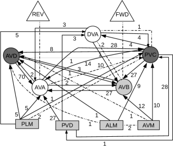
Figure 1: Tap Withdrawal Circuit of C. Elegans. Rectangle: Sensory Neurons; Circle: Inter-neurons; Dashed Undirected Edge: Gap Junction; Solid Directed Edge: Chemical Synapse; Edge Label: Number of Connections; Dark Gray: Excitatory Neuron; Light Gray: Inhibitory Neuron; White: Unknown Polarity. FWD: Forward Motor system; REV: Reverse Motor System.

The TW circuit produces three distinct locomotive behaviors: acceleration, reversal of movement, and a lack of response. In [15], Wicks et al. performed a series of laser ablation experiments in which they knocked out a neuron in a group of animals (worms), subjected them to a tapped surface, and recorded the magnitude and direction of the resulting behavior. In the control group with no neurons knocked out, 98% of subjects reacted to a tap with a reversal of locomotion, but there were still measured cases of acceleration and “no response” behavior. Fig. 2 shows the response types for each of their experiments.

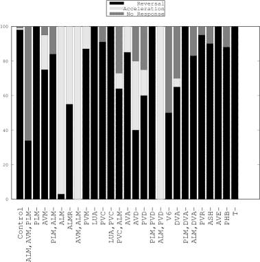
Figure 2: Effect of ablation on Tap Withdrawal reflex. The length of the bars indicate the fraction of the population demonstrating the particular behavior.

The dynamics of a neuron’s membrane potential, V, is determined by the sum of all input currents, written as:

$$C_{m}\dot{V}=\frac{1}{R_{m}}(V_{l}-V)+\sum{I^{gap}}+\sum{I^{syn}}+I^{stim}$$

where $C_{m}$ is the membrane capacitance, $R_{m}$ is the membrane resistance, $V_{l}$ is the leakage potential, $I^{gap}$ and $I^{syn}$ are gap-junction and the chemical synapse currents, respectively, and $I^{stim}$ is the applied external stimulus current. The summations are over all neurons with which this neuron has a (gap-junction or synaptic) connection.

The current flow between neuron $i$ and $j$ via a gap-junction is given by:

$$I_{ij}^{gap}=n^{gap}_{ij}g^{gap}_{m}(V_{j}-V_{i})$$

where the constant $g^{gap}_{m}$ is the maximum conductance of the gap junction, and $n^{gap}_{ij}$ is the number of gap-junction connections between neurons $i$ and $j$. The conductance $g^{gap}_{m}$ is one of the key circuit parameters of this model that dramatically affects the behavior of the animal.

The synaptic current flowing from pre-synaptic neuron $j$ to post-synaptic neuron $i$ is described as follows:

$$I_{ij}^{syn}=n^{syn}_{ij}g^{syn}_{ij}(t)(E_{j}-V_{i})$$

where $g^{syn}_{ij}(t)$ is the time-varying synaptic conductance of neuron $i$, $n^{syn}_{ij}$ is the number of synaptic connections from neuron $j$ to neuron $i$, and $E_{j}$ is the reversal potential of neuron $j$ for the synaptic conductance.

The chemical synapse is characterized by a synaptic sign, or polarity, specifying if said synapse is excitatory or inhibitory. The value of $E_{j}$ is assumed to be constant for the same synaptic sign; its value is higher if the synapse is excitatory rather than inhibitory.

Synaptic conductance is dependent only upon the membrane potential of presynaptic neuron $V_{j}$, given by:

$$g^{syn}_{ij}(t)=g^{syn}_{\infty}(V_{j})$$

where $g^{syn}_{\infty}$ is the steady-state post-synaptic conductance in response to a pre-synaptic membrane potential.

The steady-state post-synaptic membrane conductance is modeled as:

$$g^{syn}_{\infty}(V_{j})=\frac{g^{syn}_{m}}{1+\exp{(-4.3944\frac{V_{j}-V_{EQ_{j}}}{V_{Range}})}}$$

where $g^{syn}_{m}$ is the maximum post-synaptic membrane conductance for the synapse, $V_{EQ_{j}}$ is the pre-synaptic equilibrium potential, and $V_{Range}$ is the pre-synaptic voltage range over which the synapse is activated.

Combining all of the above pieces, the mathematical model of the TW circuit is a system of nonlinear ODEs, with each state variable defined as the membrane potential ofa neuron in the circuit. Consider a circuit with $N$ neurons. The dynamics of the $i^{th}$ neuron of the circuit is given by:

$$C_{m_{i}}\dot{V_{i}}=\frac{V_{l_{i}}-V_{i}}{R_{m_{i}}}+\sum_{j=1}^{N}{I_{ij}^{gap}}+\sum_{j=1}^{N}{I_{ij}^{syn}}+I^{stim}_{i}$$ (1)

$$I^{gap}_{ij}=n^{gap}_{ij}g^{gap}_{m}(V_{j}-V_{i})$$ (2)

$$I^{syn}_{ij}=n^{syn}_{ij}g^{syn}_{ij}(E_{j}-V_{i})$$ (3)

$$g^{syn}_{ij}=\frac{g^{syn}_{m}}{1+\exp{(-4.3944\frac{V_{j}-V_{EQ_{j}}}{V_{Range}})}}.$$ (4)

The equilibrium potentials ($V_{EQ}$) of the neurons are computed by setting the left-hand side of Eq. (1) to zero. This leads to a system of linear equations, that can be solved as follows:

$$V_{EQ}=A^{-1}b$$ (5)

where matrix $A$ is given by:

$$A_{ij}=\begin{cases}-R_{m_{i}}n^{gap}_{ij}g^{gap}_{m}&\text{if }i\neq j\\ 1+R_{m_{i}}\sum_{j=1}^{N}{n^{gap}_{ij}g^{gap}_{ij}g^{syn}_{m}/2}&\text{if }i=j\end{cases}$$

and vector $b$ is written as:

$$b_{i}=V_{l_{i}}+R_{m_{i}}\sum_{j=1}^{N}{E_{j}n^{syn}_{ij}g^{syn}_{m}/2}.$$

The potential of the motor neurons AVB and AVA determine the observable behavior of the animal. If the integral of the difference between $V_{\mathit{AVA}}$ - $V_{\mathit{AVB}}$ is large, the animal will reverse movement. By extension, if the difference is a large negative value, the animal will accelerate, and if the difference is close to zero there will be no response. The equation that converts the membrane potential of AVB and AVA to a behavioral property, (e.g. reversal), is given by:

$$\text{Propensity to Reverse}\propto\int(V_{\mathit{AVA}}-V_{\mathit{AVB}})dt$$ (6)

where the integration is computed from the beginning of tap stimulation until either the simulation ends or the integrand changes sign. To allow initial transients after the tap, the test for a change of integrand sign occurs only after a grace period of 100 ms.

For the purpose of reachability analysis (Section 4), we normalize the system of equations with respect to the capacitance. Combining Eqs.( 1) and ( 4) and taking $C_{m_{i}}$ to the right-hand side, we have:

$$\dot{V_{i}}=\frac{V_{l_{i}}-V_{i}}{R_{m_{i}}C_{m_{i}}}+\frac{g^{gap}_{m}}{C_{m_{i}}}\sum_{j=1}^{N}{n^{gap}_{ij}(V_{j}-V_{i})}+\frac{g^{syn}_{m}}{C_{m_{i}}}\sum_{j=1}^{N}{\frac{n^{syn}_{ij}(E_{j}-V_{i})}{1+\exp{(-4.3944\frac{V_{j}-V_{EQ_{j}}}{V_{Range}})}}}+\frac{1}{C_{m_{i}}}I^{stim}_{i}$$

Now letting $g^{leak}_{i}=\frac{1}{R_{m_{i}}C_{m_{i}}}$, $g^{gap}_{i}=\frac{g^{gap}_{m}}{C_{m_{i}}}$, $g^{syn}_{i}=\frac{g^{syn}_{m}}{C_{m_{i}}}$ and $I^{ext}_{i}=\frac{1}{C_{m_{i}}}$ the system dynamics can be written as:

$$\dot{V_{i}}=g^{leak}_{i}(V_{l_{i}}-V_{i})+g^{gap}_{i}\sum_{j=1}^{N}{n^{gap}_{ij}(V_{j}-V_{i})}+g^{syn}_{i}\sum_{j=1}^{N}{\frac{n^{syn}_{ij}(E_{j}-V_{i})}{1+\exp{(-4.3944\frac{V_{j}-V_{EQ_{j}}}{V_{Range}})}}}+I^{ext}_{i}$$ (7)

This is the 9 dimensional ODE model of the TW circuit. The key circuit parameters are the gap conductances, $g_{i}^{gap}$, and we aim to characterize the ranges of these conductances that produce acceleration, reversal, and no response.

4 Reachability Analysis of Nonlinear TW Circuit

Reachability analysis for verifying properties for general nonlinear dynamical systems is a well-known hard problem. Our approach relies on a recent line of investigation that combines static analysis of the model with validated numerical simulations [3, 9, 4].

4.1 Background on Reachability using Discrepancy

Consider an $n$-dimensional autonomous dynamical system:

$$\dot{x}=f(x),$$ (8)

where $f:{\mathbb{R}}^{n}\rightarrow{\mathbb{R}}^{n}$ is a Lipschitz continuous function. A solution or a trajectory of the system is a function $\xi:{\mathbb{R}}^{n}\times{{\mathbb{R}}_{\geq 0}}\rightarrow{\mathbb{R}}^{n}$ such that for any initial point $x_{0}\in{\mathbb{R}}^{n}$ and at any time $t>0$, $\xi(x_{0},t)$ satisfies the differential equation (8). A state $x$ in ${\mathbb{R}}^{n}$ is reachable from the initial set $\Theta\subseteq{\mathbb{R}}^{n}$ within a time interval $[t_{1},t_{2}]$ if there exists an initial state $x_{0}\in\Theta$ and a time $t\in[t_{1},t_{2}]$ such that $x=\xi(x_{0},t)$. The set of all reachable states in the interval $[t_{1},t_{2}]$ is denoted by ${\sf Reach}(\Theta,[t_{1},t_{2}])$. If $t_{1}=0$, we write ${\sf Reach}(t_{2})$ when set $\Theta$ is clear from the context. If we can compute or approximate the reach set of such a model, then we can check for invariant or temporal properties of the model. Specifically, C. Elegans TW properties such as accelerated forward movement or reversal of movement fall into these categories. Our core reachability algorithm [3, 9, 4] uses a simulation engine that gives sampled numerical simulations of (8).

Definition 1

A $(x_{0},\tau,\epsilon,T)$-simulation of (8) is a sequence of time-stamped sets $(R_{0},t_{0})$, $(R_{1},t_{1})\ldots,(R_{n},t_{n})$ satisfying:

1. Each $R_{i}$ is a compact set in ${\mathbb{R}}^{n}$ with $\mathit{dia}(R_{i})\leq\epsilon$.

2. The last time $t_{n}=T$ and for each $i$, $0<t_{i}-t_{i-1}\leq\tau$, where the parameter $\tau$ is called the sampling period.

3. For each $t_{i}$, the trajectory from $x_{0}$ at $t_{i}$ is in $R_{i}$, i.e., $\xi(x_{0},t_{i})\in R_{i}$, and for any $t\in[t_{i-1},t_{i}]$, the solution $\xi(x_{0},t)\in hull(R_{i-1},R_{i})$.

The algorithm for reachability analysis uses a key property of the model called a discrepancy function.

Definition 2

A uniformly continuous function $\beta:{\mathbb{R}}^{n}\times{\mathbb{R}}^{n}\times{{\mathbb{R}}_{\geq 0}}\rightarrow{{\mathbb{R}}_{\geq 0}}$ is a discrepancy function of (8) if

1. for any pair of states $x,x^{\prime}\in{\mathbb{R}}^{n}$, and any time $t>0$,

   $$\|\xi(x,t)-\xi(x^{\prime},t)\|\leq\beta(x,x^{\prime},t),\mbox{and}$$ (9)

2. for any $t$, as $x\rightarrow x^{\prime}$, $\beta(.,.,t)\rightarrow 0$.

If a function $\beta$ meets the two conditions for any pair of states $x,x^{\prime}$ in a compact set $K$ then it is called a $K$-local discrepancy function. Uniform continuity means that $\forall\epsilon>0,\forall x,x^{\prime}\in K,\exists\delta$ such that for any time $t,\|x-x^{\prime}\|<\delta\Rightarrow\beta(x,x^{\prime},t)<\epsilon.$ The verification results in [3, 9, 5, 4] required the user to provide the discrepancy function $\beta$ as an additional input for the model. A Lipschitz constant of the dynamic function $f$ gives an exponentially growing $\beta$, contraction metrics [12] can give tighter bounds for incrementally stable models, and sensitivity analysis gives tight bounds for linear systems [2], but none of these give an algorithm for computing $\beta$ for general nonlinear models. Therefore, finding the discrepancy can be a barrier in the verification of large models like the TW circuit.

Here, we use Fan and Mitra’s recently developed approach that automatically computes local discrepancy along individual trajectories [6]. Using the simulations and discrepancy, the reachability algorithm for checking properties proceeds as follows: Let the ${\sf U}$ be the set of states that violate the invariant in question. First, a $\delta$-cover ${\cal C}$ of the initial set $\Theta$ is computed; that is, the union of all the $\delta$-balls around the points in ${\cal C}$ contain $\Theta$. This $\delta$ is chosen to be large enough so that the cardinality of ${\cal C}$ is small. Then the algorithm iteratively and selectively refines ${\cal C}$ and computes more and more precise over-approximations of ${\sf Reach}(\Theta,T)$ as a union $\cup_{x_{0}\in{\cal C}}{\sf Reach}(B_{\delta}(x_{0}),T)$. Here, ${\sf Reach}(B_{\delta}(x_{0}),T)$ is computed by first generating a $(x_{0},\tau,\epsilon,T)$-simulation and then bloating it by a factor that maximizes $\beta(x,x^{\prime},t)$ over $x,x^{\prime}\in B_{\delta}(s_{0})$ and $t\in[t_{i-1},t_{i}]$. If ${\sf Reach}(B_{\delta}(x_{0}),T)$ is disjoint from ${\sf U}$ or is (partly) contained in ${\sf U}$, then the algorithm decides that $B_{\delta}(x_{0})$ satisfies and violates ${\sf U}$, respectively. Otherwise, a finer cover of $B_{\delta}(x_{0})$ is added to ${\cal C}$ and the iterative selective refinement continues. We refer to this in this paper as $\delta$-refinement. In [3], it is shown that this algorithm is sound and relatively complete for proving bounded time invariants.

4.2 Applying Local Discrepancy to TW Circuit

Fan and Mitra’s algorithm (see details in [6]) for automatically computing local discrepancy relies on the Lipschitz constant and the Jacobian of the dynamic function, along with simulations. The Lipschitz constant is used to construct a coarse, one-step over-approximation $S$ of the reach set of the system along a simulation. Then the algorithm computes an upper bound on the maximum eigenvalue of the symmetric part of the Jacobian over $S$, using a theorem from matrix perturbation theory. This gives a piecewise exponential $\beta$, but the exponents are tight as they are obtained from the maximum eigenvalue of the linear approximation of the system in $S$. This means that for models with convergent trajectories, the exponent of $\beta$ over $S$ will be negative, and the ${\sf Reach}(T)$ approximation will quickly become very accurate. In the rest of this section, we describe key steps involved in making this approach work with the TW circuit.

The model of the TW circuit from Section 3 can be written as $\dot{V}=f(V)$, where $V\in{\mathbb{R}}^{9}$. The Jacobian of the system is the matrix of partial derivatives with the $ij^{th}$ term given by:

$$\frac{\partial f_{i}}{\partial V_{i}} = -g_{i}^{leak}-g_{i}^{gap}\sum_{j=1,j\neq i}^{N}n_{ij}^{gap}-g_{i}^{syn}\sum_{j=1,j\neq i}^{N}\frac{n_{ij}^{syn}}{1+\exp(-4.3944\frac{V_{j}-V_{EQ_{j}}}{V_{Range}})}$$ (10)

$$= g_{i}^{gap}n_{ij}^{gap}-g_{i}^{syn}n_{ij}^{syn}\frac{\frac{-4.3944}{V_{Range}}\exp(-4.3944\frac{V_{j}-V_{EQ_{j}}}{V_{Range}})(E_{j}-V_{i})}{(1+\exp(-4.3944\frac{V_{j}-V_{EQ_{j}}}{V_{Range}}))^{2}}$$

For parameter-range estimation of the TW circuit, each parameter $p$ of interest is added as a new variable with constant dynamics ($\dot{p}=0$). Computing the reach-set from initial values of $p$ is then used to verify or falsify invariant properties for a continuous range of parameter values, and therefore a whole family of models, instead of analyzing just a single member of that family. Here the parameters of interest are the quantities $1/g_{i}^{leak},10/g_{i}^{gap},1/g_{i}^{syn}$. Consider, for example, $1/g_{i}^{leak}$ as a parameter:

$$\dot{\left[\begin{array}[]{c}V\\ 1/g_{i}^{leak}\end{array}\right]}=\left[\begin{array}[]{c}f(V)\\ 0\end{array}\right].$$

In this case the Jacobian matrices for the system with parameters will be singular because of the all-zero rows that come from the parameter dynamics. The zero eigenvalues of these singular matrices are taken into account automatically by the algorithm for computing local discrepancy. In this paper we focus on $10/g_{i}^{gap}$, leaving the others for future work.

4.3 Checking Properties

Once the reach sets are computed, checking the acceleration, reversal, and no-response properties are conceptually straightforward. For instance, Equation (6) gives a method to check reversal movement. Instead of computing the integral of $({V_{\mathit{AVA}}-V_{\mathit{AVB}}})$, we use the following sufficient condition to check it:

$$\forall\ t\in T_{\mathit{int}},\forall\ x\in{\sf Reach}(\Theta,[t,t]),V_{\mathit{AVA}}(x)>V_{\mathit{AVB}(x)}.$$

Here, $T_{int}$ is a specific time interval after the stimulation time, $\Theta$ is the initial set with parameter ranges, and recall that ${\sf Reach}(\Theta,[t,t])$ is the set of states reached at time $t$ from $\Theta$. We implement this check by scanning the entire reachtube and checking that its projection on $V_{\mathit{AVB}}(x)$ is above that of $V_{\mathit{AVA}}(x)$ over all intervals. If this check succeeds (as in Figure 4(a)), we conclude that the range of parameter values produce the reversal movement. If the check fails, then the reversal movement is not provably satisfied (Figure 4(b)) and in that case we $\delta$-refine the initial partition.

(a) Rev. property satisfied with $g^{gap}_{AVM}=1000$.

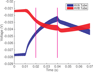
(b) Rev. unknown with $g^{gap}_{AVM}=33.33$.

Figure 3: Model Checking Reversal Property of Control Group, with $\delta=5e-5$, varying $g^{gap}_{\mathit{AVM}}$.

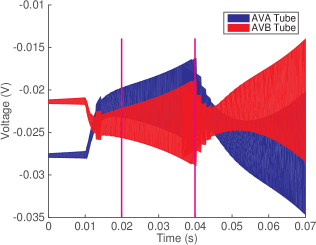
(a) Rev. property unknown with $\delta=1e$-$4$.

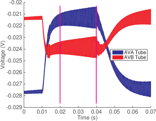
(b) Rev. property satisfied with $\delta=5e$-$5$.

Figure 4: Model Checking Reversal Property of Control Group by refining $\delta$.

5 Experimental Results

In this section, we apply reachability analysis to parameter rangers that produce three different behaviors (reversal, acceleration, no response) in the control and four ablation groups. When a tap stimulus is applied, the sensory neurons (ALM, AVM and PLM) propagate that signal to the motor neurons via interneurons. The gap-junctions formed by the sensory neurons are the most important functional connections to this process [1]. Therefore we vary only the gap-junction conductance, $g^{gap}_{i}$, of the sensory neurons and keep all other parameters constant, as per [16]. Our experiments characterize parameter ranges for reversal, acceleration and no response behaviors in all groups, except the ALM,AVM- group where reversal behavior is not observed.

In section 4, we explain that we use $10/g^{gap}_{i}$ as our parameter in the state vector instead of $g^{gap}_{i}$. Assume $p^{gap}_{i}=10/g^{gap}_{i}$, $i\in\{AVM,ALM,PLM\}$. The corresponding range for $p^{gap}_{i}$ is $[0.01,1]$. From the reachability analysis, we estimate ranges for $p^{gap}_{i}$ that can be converted back to $g^{gap}_{i}$.

In the following subsections, we will present our results for parameter range estimation for all three behaviors of the control and ablation groups. This process requires three experiments per group.

5.1 1-D Parameter Space

Here we vary one conductance at a time for two groups: the control and the ALM, AVM ablation groups.

5.1.1 Control:

For the control case, we varied $p^{gap}_{\mathit{AVM}}$. We found that the reversal property is satisfied in sub-range $[0.01,0.214]$ with $\delta=1e-6$ and the acceleration property in sub-range $[0.63,1]$ with $\delta=1e-5$. Recall, $\delta$ is the size of the finest cover used by the verification algorithm. We could not verify any property for the sample points in sub-range $(0.214,0.63)$. As shown in Table 1, the parameter range producing reversal, as identified by our procedure, dominates the parameter range for acceleration. Our procedure also shows that no value of $p^{gap}_{AVM}$ produces the no-response behavior for the control group.

The time required for our procedure is dependent upon the property, the interval for each dimension, and the size of $\delta$. For example, the time necessary to complete the procedure for the reversal property is approximately one hour.

5.1.2 ALM, AVM Ablation Group:

In this group two sensory neurons, ALM, and AVM, are ablated. As such, we vary only $p^{gap}_{\mathit{PLM}}$. Acceleration is satisfied over the interval $[0.01,0.3]$ with $\delta=5e-5$ and no response behavior is satisfied over $[0.75,1]$ with the same $\delta$. Despite using a very small $\delta$ for refinement, we did not observe any reversal behavior in this entire range. Examining Table 1 we see that acceleration is the dominant behavior for this group.

5.2 2-D Parameter Space

We lead with results for the control group, then examine various ablation groups.

5.2.1 Parameter Refinement in 2-D:

Fig. 5 helps paint a picture of how the $\delta$-refinement process discussed in Section 4 works in 2-D. We consider 4 refinement steps for the control group: $\delta=7e-5$, $\delta=6e-5$, $\delta=5.5e-5$, and $\delta=5e-5$. For $\delta=7e-5$, the property of interest is unknown at all points. With $\delta=6e-5$ the property is considered unknown for all red areas in the figure, including red and blue areas. Blue areas show where $\delta=5.5e-5$ are satisfied, and in the blue and yellow area both $\delta=6e-5$ and $\delta=5.5e-5$ have a satisfied property. The property is satisfied for the entire range of the graph when $\delta=5e-5$. Thus, the refinement process stops at $\delta=5e-5$, and the entire range of the 2-D parameter space is characterized.

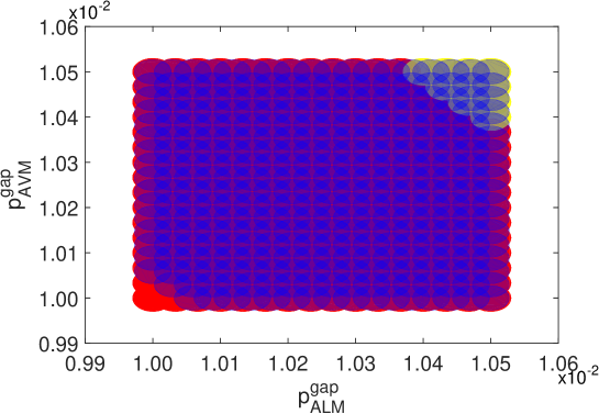
Figure 5: Example of 2-D Parameter Refinement. Red Regions are Unknown for both $\delta=6e-5$ and $\delta=5.5e-5$, Red/Blue Regions are Unknown for $\delta=6e-5$, but Satisfied for $\delta=5.5e-5$, and Yellow/Blue Regions are Satisfied for both.

5.2.2 Control

Here we consider the $p^{gap}_{\mathit{AVM}}$ and $p^{gap}_{\mathit{ALM}}$ conductances simultaneously. For this group, reversal is satisfied over the range $[0.01,0.0105]$ with $\delta=2e-5$ and acceleration is satisfied over $[0.63,0.6305]$ with the same $\delta$. Table 1 shows that reversal, like in the 1-D case, dominates and no response is not generated.

Table 1: Regions in the parameter space in which the properties are proven satisfied. A 1-D case shows interval size, a 2-D case shows area, and a 3-D case shows volume.

5.2.3 PLM Ablation Group:

As the PLM neuron is ablated in this group, varying only $p^{gap}_{\mathit{AVM}}$ and $p^{gap}_{\mathit{ALM}}$ is sufficient to produce all three behaviors. Here we find reversal satisfied over $[0.01,0.0105]$ with $\delta=2e-5$, acceleration over $[0.67,0.6705]$ with $\delta=5e-5$, and no response over $[0.9995,1]$ with $\delta=5e-5$. Table 1 shows that reversal dominates the other two behaviors, but all three are produced.

5.2.4 ALM Ablation Group:

To produce all three behaviors of this group we vary only $p^{gap}_{\mathit{AVM}}$ and $p^{gap}_{\mathit{PLM}}$. Reversal is satisfied over the interval $[0.01,0.0105]$ with $\delta=5e-5$, acceleration over $[0.67,0.6705]$ with $\delta=2e-5$, and no response over $[0.9995,1]$ with $\delta=5e-5$. We can see in Table 1 that this ablation group has a propensity to reverse. The astute reader would notice that this trend does not seem to match Fig. 2, unlike the rest of our results. We have run simulations with the equations from  [16], and the simulations also produce reversal, not acceleration. The results of the simulation and model checking consistently disagree with the behavior denoted in Fig. 2 for this ALM group. We are currently investigating why this is the case.

5.2.5 ALM, DVA Ablation Group:

All three behaviors of this group are produced by varying only $p^{gap}_{\mathit{AVM}}$ and $p^{gap}_{\mathit{PLM}}$. Here reversal is satisfied over $[0.02,0.0205]$ with $\delta=2e-5$, acceleration over $[0.67,0.6705]$ with $\delta=5e-5$, and no response over $[0.9995,1]$ with $\delta=5e-5$. Repeating our experiments for this group, Table 1 shows the dominant reversal behavior.

5.3 3-D Parameter Space

Since the ablation groups we have used in this paper all feature at least one of the primary sensory neurons (ALM, AVM, and PLM) ablated, we can only show the 3-D case for the original animal.

For the 3-D case, in addition to $p^{gap}_{\mathit{AVM}}$ and $p^{gap}_{\mathit{ALM}}$, we have the $p^{gap}_{\mathit{PLM}}$ conductance. Finally, we get a non-zero value for no response in the control, but Table 1 shows that this value is an order of magnitude smaller than acceleration and several orders smaller than reversal. Reversal is satisfied over $[0.01,0.0101]$ with $\delta=2e-5$, acceleration over $[0.631,0.6305]$ with $\delta=5e-5$, and no response over $[0.63,0.63005]$ with $\delta=5e-5$.

6 Conclusions

In this paper, we performed reachability analysis with discrepancy to automatically determine parameter ranges for three fundamental reactions by C. Elegans to tap-withdrawal stimulation: reversal of movement, acceleration, and no response. We followed the lead of the in vivo experimental results of [15] to obtain parameter-estimation results for gap-junction conductances for a number of neural-ablation groups. To the best of our knowledge, these results represent the first formal verification of a biologically realistic (nonlinear ODE) model of a neural circuit in a multicellular organism.

Our results are further organized into how many of these three conductances we considered simultaneously. For each of these cases, we were able to determine parameter ranges for which the three TW responses are guaranteed to hold. Moreover, with the exception of the ALM- ablation group (an exception Wicks himself has noted about the ODE circuit model), our results match the relative-percentage trends of Fig. 2.

Future work includes expanding the parameter ranges for TW responses, possibly by parallelizing the verification algorithm. We also plan to examine the additional ablation groups present in Fig. 2.

Acknowledgments.

We would like to thank Junxing Yang, Heraldo Memelli, Farhan Ali, and Elizabeth Cherry for their numerous contributions to this project. Our research is supported in part by the following grants: NSF IIS 1447549, NSF CAR 1054247, AFOSR FA9550-14-1-0261, AFOSR YIP FA9550-12-1-0336, CCF-0926190, and NASA NNX12AN15H.

References

- [1] M. Chalfie, J. E. Sulston, J. G. White, E. Southgate, J. N. Thomson, and S. Brenner. The neural circuit for touch sensitivity in Caenorhabditis Elegans. The Journal of Neuroscience, 5(4):956–964, 1985.
- [2] A. Donzé and O. Maler. Systematic simulation using sensitivity analysis. In Hybrid Systems: Computation and Control, pages 174–189. Springer, 2007.
- [3] P. S. Duggirala, S. Mitra, and M. Viswanathan. Verification of annotated models from executions. In Proceedings of the International Conference on Embedded Software, EMSOFT 2013, Montreal, Canada, Sep.-Oct. 2013. IEEE.
- [4] P. S. Duggirala, S. Mitra, M. Viswanathan, and M. Potok. C2E2: A verification tool for Stateflow models. In 21st International Conference on Tools and Algorithms for the Construction and Analysis of Systems, TACAS 2015, 2015.
- [5] P. S. Duggirala, L. Wang, S. Mitra, M. Viswanathan, and C. Muñoz. Temporal precedence checking for switched models and its application to a parallel landing protocol. In FM 2014: Formal Methods, 19th International Symposium, Proceedings, volume 8442 of Lecture Notes in Computer Science, pages 215–229. Springer, May 2014.
- [6] C. Fan and S. Mitra. Bounded verification using on-the-fly discrepancy computation. Technical Report UILU-ENG-15-2201, Coordinated Science Laboratory, University of Illinois at Urbana-Champaign, Feb. 2015.
- [7] R. Grosu, G. Batt, F. H. Fenton, J. Glimm, C. L. Guernic, S. A. Smolka, and E. Bartocci. From cardiac cells to genetic regulatory networks. In Proceedings of the 23rd International Conference on Computer Aided Verification, pages 396–411. Springer, 2011.
- [8] A. L. Hodgkin and A. F. Huxley. A quantitative description of membrane current and its application to conduction and excitation in nerve. Journal of Physiology, 117:500–544, 1952.
- [9] Z. Huang, C. Fan, A. Mereacre, S. Mitra, and M. Z. Kwiatkowska. Invariant verification of nonlinear hybrid automata networks of cardiac cells. In Computer Aided Verification, 26th International Conference, CAV 2014, Proceedings, volume 8559 of Lecture Notes in Computer Science, pages 373–390, Vienna, Austria, July 2014. Springer.
- [10] M. A. Islam, A. Murthy, A. Girard, S. A. Smolka, and R. Grosu. Compositionality results for cardiac cell dynamics. In Proceedings of the 17th International Conference on Hybrid Systems: Computation and Control. ACM, 2014.
- [11] S. M. Iyengar, C. Talcott, R. Mozzachiodi, E. Cataldo, and D. A. Baxter. Executable symbolic models of neural processes. Network Tools and Applications in Biology (NETTAB07), 2007.
- [12] W. Lohmiller and J. J. E. Slotine. On contraction analysis for non-linear systems. Automatica, 1998.
- [13] A. Murthy, M. A. Islam, R. Grosu, and S. A. Smolka. Computing bisimulation functions using SOS optimization and delta-decidability over the reals. In Proceedings of the 18th International Conference on Hybrid Systems: Computation and Control. ACM, 2015.
- [14] A. Tiwari and C. L. Talcott. Analyzing a discrete model of Aplysia central pattern generator. In Proceedings of the 6th Conference on Computational Methods in Systems Biology (CMSB), pages 347–366. Springer, 2008.
- [15] S. R. Wicks and C. H. Rankin. Integration of mechanosensory stimuli in Caenorhabditis Elegans. The Journal of Neuroscience, 15(3):2434–2444, 1995.
- [16] S. R. Wicks, C. J. Roehrig, and C. H. Rankin. A dynamic network simulation of the nematode tap withdrawal circuit: Predictions concerning synaptic function using behavioral criteria. The Journal of Neuroscience, 16(12):4017–4031, 1996.