The Physical Conditions in a Pre Super Star Cluster Molecular Cloud in the Antennae Galaxies

Abstract

We present an analysis of the physical conditions in an extreme molecular cloud in the Antennae merging galaxies. This cloud has properties consistant with those required to form a globular cluster. We have obtained ALMA CO and 870$\mu$m observations of the Antennae galaxy system with $\sim 0^{\prime\prime}.5$ resolution. This cloud stands out in the data with a radius of $\lesssim 24$ pc and mass of $>5\times 10^{6}$ M_⊙. The cloud appears capable of forming a globular cluster, but the lack of associated thermal radio emission indicates that star formation has not yet altered the environment. The lack of thermal radio emission places the cloud in an early stage of evolution, which we expect to be short-lived ($\lesssim 1$ Myr) and thus rare. Given its mass and kinetic energy, for the cloud to be confined (as its appearance strongly suggests) it must be subject to an external pressure of P/$k_{B}\gtrsim 10^{8}$ K cm^-3 – 10,000 times higher than typical interstellar pressure. This would support theories that high pressures are required to form globular clusters and may explain why extreme environments like the Antennae are preferred environments for generating such objects. Given the cloud temperature of $\sim 25$ K, the internal pressure must be dominated by non-thermal processes, most likely turbulence. We expect the molecular cloud to collapse and begin star formation in $\lesssim 1$ Myr.

1. Introduction

1.1. Globular Cluster Formation

Globular clusters are among the most ancient objects in the universe, often with ages $>12$ Gyr (Bolte & Hogan, 1995; Carretta et al., 2000) and are common around massive galaxies in the universe today (Harris et al., 2013). The present-day abundance of globular clusters is remarkable given that that the fraction expected to survive $\sim 10$ Gyr is extremely small, potentially lower than 1% (Fall & Zhang, 2001; Whitmore, Chandar, & Fall, 2007). Thus, this extreme type of star formation may have been a critical mode in the early evolution of today’s massive galaxies.

Initial theories about globular cluster formation suggested that these objects were among the first to gravitationally collapse in the early universe (Peebles & Dicke, 1968). Subsequent work, particularly after the launch of the Hubble Space Telescope, has demonstrated that clusters with extreme stellar densities often exceeding $\sim 10^{4}$ stars pc^-3 (e.g. Miocchi et al., 2013) can still form in the universe today (O’Connell et al., 1994) – the so-called “super star clusters” (SSCs). Since that time, numerous studies have indicated that the properties of SSCs are consistent with those expected of young globular clusters (e.g. McLaughlin & Fall, 2008).

A number of physical processes contribute to the destruction of clusters, including two-body relaxation, stellar mass loss and feedback, compressive and tidal shocks as clusters orbit their host galaxy, and tidal truncation. The extent to which each of these processes act on a specific cluster will depend on a variety of factors, including the orbital properties of the cluster (Gnedin & Ostriker, 1997). Indeed, the extent to which cluster disruption is mass-dependent is still debated (Fall et al., 2009; Bastian et al., 2012). For unresolved clusters in galaxies outside the local group, there is typically limited (if any) dynamical information, and for clusters younger than a few Myr, little dynamical evolution will have taken place. For all of these reasons, it is not possible to say whether any particular SSC will survive for a Hubble time.

While there is no generally accepted definition of “Super Star Cluster”, here we adopt a definition based on a cluster having the potential to evolve into a globular cluster, regardless of whether or not it actually will do so over the following $\sim$ 10 Gyr. This requirement results in both mass and radius limits on the range of objects that can be considered as SSCs. Specifically, most present-day globular clusters have half-light radii of $<10$ pc (although some have radii as large as $\sim 15$ pc, van den Bergh et al., 1991), and stellar masses of $\gtrsim 10^{5}$ M_⊙ (Harris et al., 1994). In addition, these clusters are expected to lose $\gtrsim 1/2$ of their mass due to dynamical effects over  10¹⁰ years (McLaughlin & Fall, 2008), which suggests that to be a globular cluster progenitor, a young star cluster should have a mass of $\gtrsim 2\times 10^{5}$ M_⊙. If star formation efficiency is $\sim 20-50$% (Ashman & Zepf, 2001; Kroupa et al., 2001), the initial molecular core from which the cluster is formed must have a mass of $\gtrsim 10^{6}$ M_⊙.

Optical techniques have been able to probe the evolution of SSCs (and presumably some future globular clusters) to ages as young as a few million years. Before this time, the clusters can be significantly shrouded by their birth material, limiting the usefulness of optical observations. Beginning in the late 1990’s efforts began to observe SSC evolution at even earlier ages ($\lesssim$ a few million years) by using radio observations to detect the free-free emission from the ionized gas around the cluster and internal to the cluster’s dust cocoon (Turner, Ho, & Beck, 1998; Kobulnicky & Johnson, 1999; Turner et al., 2000; Beck, Turner, & Kovo, 2000; Johnson et al., 2001; Johnson, 2002; Johnson et al., 2003; Beck et al., 2004; Turner & Beck, 2004; Johnson et al., 2004; Reines et al., 2008; Johnson, Hunt, & Reines, 2009; Tsai et al., 2009; Aversa et al., 2011; Kepley et al., 2014). We refer to these objects as “natal” SSCs, meaning that the clusters themselves have already formed, but they have not yet emerged from their birth material. Studies of natal clusters were able to place constraints on the relative lifetime of this enshrouded phase of SSC evolution to $\lesssim$ a million years and the gas density of the ionized hydrogen $n_{e}>10^{3}$ cm^-3(Johnson et al., 2003). A large number of subsequent studies have now identified additional compact thermal radio sources in a number of galaxies, although their low detection rate supports their relatively short lifetime (Tsai et al., 2009; Aversa et al., 2011).

However, determining the physical conditions that give rise to SSCs (and their surviving descendants – globular clusters) has been mired in the fundamental difficulty that once an SSC is present in the molecular cloud, it will dramatically alter it. Thus in order to observationally probe the conditions capable of creating an SSC requires not only identifying molecular clouds that are compact (radii $\lesssim 25$ pc, see Section 3.5) and massive ($\gtrsim 10^{6}$ M_⊙), but also for which massive stars have not begun to disrupt the environment. Efforts to observe the actual formation of SSCs – before the star clusters have formed – requires high spatial resolution millimeter observations to determine the physical properties of the material from which the clusters will form. Such work has largely been stymied by the available observing facilities and limited to only the most nearby galaxies.

One example of a relatively nearby starburst system in which some progress has been made is M82. At 3.6 Mpc (Freedman et al., 1994), relatively good linear resolution was achievable even before ALMA. This system was observed using the Owens Valley Radio Observatory (OVRO) in CO(2-1) with a linear resolution of 17 pc Keto et al. (2005). While the compact molecular clouds observed in M82 are likely to be associated with early SSC evolution, multiwavelength observations suggest that these clouds have already begun star formation (Keto et al., 2005), and have therefore disrupted their birth environment.

This paper reports results from an ALMA Early Science project studying the Antennae galaxies. In a high resolution survey of CO emission from the Antennae (Whitmore et al., 2014) the most immediately striking feature was a compact, high line width cloud with little associated star formation. This is coincident with a source identified by Herrera et al. (2011, 2012) as a potential proto-SSC using H₂ and earlier, lower resolution ALMA data. The strong compact H₂ emission appears to be due to warm (1700-2300 K) shocked gas. However, the size of the cold molecular component could only be constrained to $\lesssim 100$ pc, which precluded a conclusive identification.

The present paper characterizes this source, which we consider among the best candidates for a proto-SSC, and lays out the evidence for and against the source’s eventual evolution into a SSC or GC.

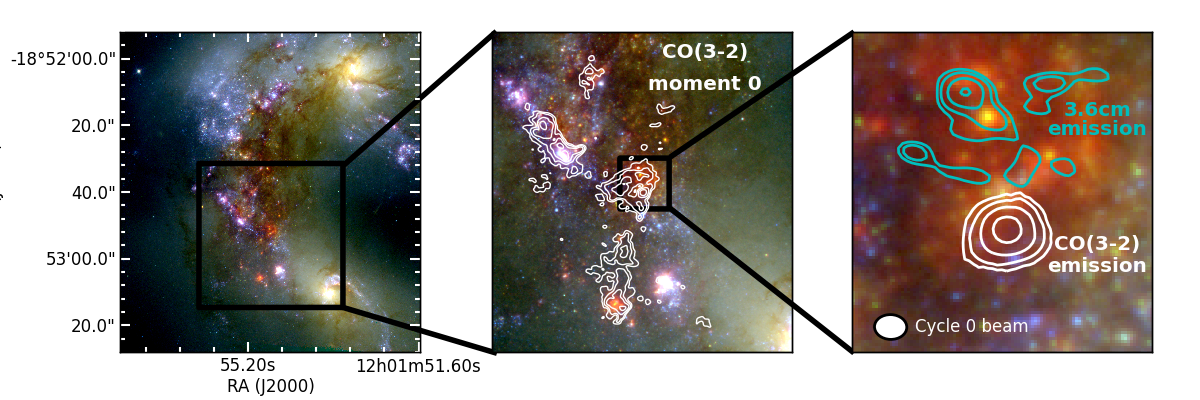
Figure 1.— The candidate proto super star cluster molecular cloud is located in the “Overlap” region of the Antennae merging galaxies. (left) HST color image of the central area of the Antennae Overlap region (red = Pa$\alpha$, green = F814W ($\sim$ I-band), blue = F435W ($\sim$B-band)), (middle) A magnified view of the “overlap” region overlaid with contours (2, 4, 8, and 16 Jy beam^-1 km s^-1) from the ALMA Cycle 0 CO(3-2) moment 0 map. (right) A zoomed-in view of the region surrounding the candidate proto super star cluster molecular cloud overlaid with both CO(3-2) contours of the molecular cloud after extraction from the data cube (0.4, 0.8, 1.6, 3.2 Jy beam^-1 km s^-1) and 3.6cm radio emission (-1, 4, 5, 7, 10$\sigma$, $\sigma=3.8\times 10^{-2}$ mJy beam^-1). The synthesized beam, shown in the right panel, has a size of $0.^{\prime\prime}56\times 0.^{\prime\prime}43$.

Table 1Interferometric CO Observations of the Antennae

Facility	Transition	Beam	Reference
CMA	12CO1-0	$4.91^{\prime\prime}\times 3.15^{\prime\prime}$	Wilson et al. (2000)
SMA	12CO3-2	$1.42^{\prime\prime}\times 1.12^{\prime\prime}$	Ueda et al. (2012)
SMA+PdBI	12CO2-1	$3.3^{\prime\prime}\times 1.5^{\prime\prime}$	Wei et al. (2012)
ALMA-SV	12CO2-1	$1.68^{\prime\prime}\times 0.85^{\prime\prime}$	Espada et al. (2012)
ALMA-SV	12CO3-2	$1.05^{\prime\prime}\times 0.60^{\prime\prime}$	Herrera et al. (2012)
ALMA-Cyc0	12CO3-2	$0.56^{\prime\prime}\times 0.43^{\prime\prime}$	this paper

2. ALMA Observations

We obtained ALMA observations of the Antennae system in CO(3-2) and 870$\;\mu$m continuum with the goal of probing the conditions of cluster formation and early evolution; data calibration is discussed in detail in the overview paper (Whitmore et al., 2014). Briefly, the observations consisted of a 13-point mosaic, and were carried out in the “extended” configuration, with a maximum baseline of $\sim 400$ m and 5 km s^-1 spectral channels. The resulting rms was determined using line-free channels and found to be 3.3 mJy/beam. With an angular resolution FWHM of $0.^{\prime\prime}56\times 0.^{\prime\prime}43$ ($59\times 45$ pc), these observations are well-matched to the expected diameter of the precursor giant molecular clouds of $\lesssim 50$ pc (or a radius of 25 pc, see Section 3.5). For this paper, we also recalibrated and reimaged the SV data, as well as compared it to previous results to check for consistency. The SV CO(2-1) data used in this paper was taken with a beam size of $1.68^{\prime\prime}\times 0.85^{\prime\prime}$. The rms of the SV CO(2-1) observations was also measured using line-free channels and found to be 6.5 mJy/beam.

The ALMA observations enable the study of a compact and luminous source in the CO(3-2) data cube (see Figure 1). This cloud is part of the super giant molecular cloud complex known as SGMC2 (Wilson et al., 2000); the full 3-D cube of SGMC2 is shown in Figure 2. The Antennae galaxy system was previously observed in both CO(2-1) and CO(3-2) by ALMA as part of the “science verification” (SV) process, which has already resulted in publications (see Table 1, Espada et al., 2012; Herrera et al., 2012).

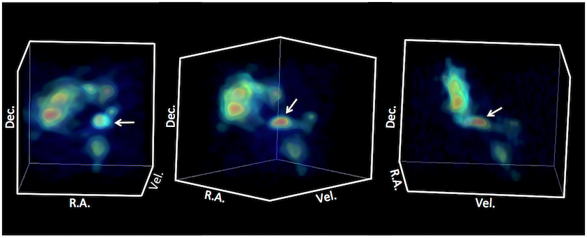
Figure 2.— A 3-D view of the data cube illustrates the spatial and velocity structure of the entire SGMC2 region. The candidate proto-super star cluster molecular cloud is indicated by the arrow, and the secondary cloud is spatially offset slightly to the north-west; the primary cloud stands out in the data cube due to its round shape, compact size, and larger velocity dispersion (it is visibly extended in velocity space, in contract to other clouds in the cube, including the secondary cloud which is offset to higher velocity). The spatial dimensions of the cube are $9.^{\prime\prime}6\times 9.^{\prime\prime}6$, and the velocity axis spans 1300-1800 km s^-1.

The specific source discussed here was singled out in the lower-resolution ALMA science verification data, with the CO(3-2) emission being coincident with strong H₂ emission – potentially indicating shocks due to infalling gas (Herrera et al., 2012). Even with lower resolution data ($\sim 100$ pc), it was speculated that this region might contain an SSC in the early stages of its evolution (Herrera et al., 2012). However, the spatial resolution of the SV CO(3-2) data is $\sim 100$ pc, or roughly twice that of the Cycle 0 data presented here. It is clear that in the SV data, the molecular cloud that is the subject of this paper is not resolved and is blended with other molecular material in the vicinity.

Table 2Measured Properties of the Molecular Cloud

R.A.	Dec.	VLSR	SCO3-2	$\sigma_{V}$	Size
(J2000)	(J2000)	(km s-1)	(Jy km s-1)	(km s-1)	FWHM (arcsec2)
12:01:54.73	-18:52:53.2	1524$\pm 3$	52$\pm 5$	49$\pm 3$	$0.66\pm 0.12\times 0.55\pm 0.07$

Note. — Properties of the clouds were measured both with the CPROPS program Rosolowsky & Leroy (2006), and with Gaussian fitting (FWHM $=2.35\sigma$). The quoted uncertainties reflect empirically determined variations in these values for different fitting attempts. The synthesized beam has $\it not$ been deconvolved in this table to strictly report measured properties. The deconvolved size is reported in Table 3.

2.1. Cloud Analysis

Determining the properties of this cloud requires that it first be isolated from other emission in the region. As shown in Figures 3 and 4, there is a redshifted secondary velocity component along this line of sight, that must be deconvolved from the primary source before analysis. We extract the primary cloud from the velocity cube for further analysis by creating a sub-cube around the cloud with dimensions of $\sim 1^{\prime\prime}\times 1^{\prime\prime}\times 300$ km s^-1. The integrated intensity contours of the extracted primary cloud are shown in Figure 1, and the observed properties are listed in Table 2. We determine the cloud size by deconvolving the synthesized beam from the extracted source, which yields a half-light radius for the cloud of $\lesssim 24\pm 3$ pc ($\lesssim 0.23^{\prime\prime}$). The derived properties of the cloud are given in Table 2. As a sanity check, the properties of the primary cloud were also determined using the CPROPS program on the entire data cube (not exclusively the sub-cube) (Rosolowsky & Leroy, 2006), and the resulting parameters agree to within the uncertainties. Thus, by-hand measurement of the half-light size, automated Gaussian fits, and moment based measurements all yield roughly consistent sizes for our cloud. As this is a marginally resolved object with a clearly measurable line width methodological uncertainties do not overwhelm any of our conclusions. Throughout this text, we refer to the properties of the extracted primary cloud only, unless noted otherwise.

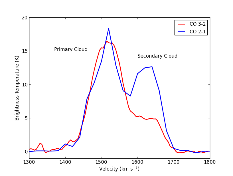
Figure 3.— The CO(3-2) and CO(1-0) spectra of a $\sim 1^{\prime\prime}\times 1^{\prime\prime}$ region around the candidate proto super star cluster molecular cloud taken from the full data cube (i.e. the primary cloud has not been extracted). The line emission indicates that there are two components along the line-of-sight that have different temperatures. Spectral profile of the CO(3-2) line from current work (ALMA Cycle 0 observations) and the CO(2-1) line from ALMA science verification (Espada et al., 2012). The CO(3-2) data is convolved to the CO(2-1) beam and both data sets are corrected for beam dilution. There is clearly more than one velocity component; in these convolved data, the secondary source was fit by a Gaussian and subtracted from the spectra. The CO(3-2)/CO(2-1) ratio is dramatically different in the two velocity components.

2.2. Relative Astrometric Solutions

A comparison between the CO(3-2) emission and data at other wavelengths, requires an understanding of the relative astrometric accuracy. Based on the phase stability of the ALMA observations, we estimate the absolute astrometric accuracy to be better than $\sim 0.2^{\prime\prime}$. Centimeter observations from the VLA have an astrometric accuracy better than $\sim 0.1^{\prime\prime}$ (Brogan et al., 2010), and therefore the 3.6 cm and CO(3-2) observations have a relative precision of better than the synthesized beam of the ALMA data, and we consider them to be astrometrically matched. We also register the astrometry of archival Hubble Space Telescope observations shown in Figure 1 by matching the Pa${\alpha}$ emission throughout the Antennae system to common features in the 3.6 cm emission.

3. Results

3.1. Cloud Temperature and Optical Depth

We constrain the temperature and optical depth of the cloud using the CO(3-2) and CO(2-1) emission. We retrieved, recalibrated, and reimaged CO(2-1) observations from ALMA’s science verification period, shown over-plotted in Figure 3. The CO(3-2) observations were convolved to the synthesized beam of the CO(2-1) observations and corrected for beam dilution using the Cycle 0 CO(3-2) source size, resulting in peak brightness temperatures of T${}_{3-2}=17\pm 3$ K and T${}_{2-1}=18\pm 3$ K. The largest angular scale to which the CO(3-2) observations are sensitive is $\sim 6^{\prime\prime}$, and therefore we do not expect that any flux is resolved out on the size scales of interest here. The secondary component has a significantly lower CO(3-2)/CO(2-1) ratio, indicating much cooler gas than the primary cloud.

RADEX non-LTE modeling (van der Tak et al., 2007) was used to analyze the CO(3-2) and CO(2-1) emission. The line intensities and their ratio were compared to a grid of RADEX models covering a range of values for kinetic temperature, CO column density, and H₂ volume density. The best-fit values result from a chi-squared minimization. Since the source is marginally resolved in CO(3-2), for CO(3-2) we set the beam filling fraction to 1, and for CO(2-1) we set it to the dilution factor, or the ratio of the CO(3-2) size to the CO(2-1) beamsize. The RADEX models indicate that these transitions are optically thick – the best fitting depth is $\tau\sim 3.5\pm 0.5$, but the data do not rule out significantly higher values. The lines appear to be close to thermalized, with an excitation temperature within a degree of the kinetic temperature of 25${}^{+10}_{-2}$ K; this temperature is on the upper end of the range of those found for dense molecular clouds in the Milky Way (Shirley et al., 2013). However, there is a degeneracy between the inferred temperature and density of the cloud, and the cloud could be warmer for densities $\lesssim 6\times 10^{4}$ cm^-3. In other words, the observed brightness could also be reproduced with a large column of subthermally excited, warm, relatively diffuse gas.

Table 3Derived Properties of the Molecular Cloud

Deconv.	Half Light	Mvirial	M${}_{X_{CO}}$	MRADEX	MCont.	TKin	$\rho$
FWHM (pc2)	R (pc2)	($10^{6}$ M⊙)	($10^{6}$ M⊙)	($10^{6}$ M⊙)	($10^{6}$ M⊙)	(K)	(g cm-3)
$<53\times 41$	$<27\times 21^{c}$	$29-85$	$3.3-15$	$>2.8$	$3.1-7.4$	$23-35$	$2-20\times 10^{-21}$

Note. — The FWHM as measured after deconvolving the synthesized beam and adopting a distance of 21.5 Mpc. The half light radius resulting from deconvolution assuming a Gaussian distribution of light. The cloud is consistent with either being marginally resolved or a point source at this resolution.

The temperature inferred here for the CO cloud is roughly 100$\times$ less than that inferred for the compact H₂ emission observed in this region of 1,700-2,300 K (Herrera et al., 2011). In addition, the H₂ FWHM line-width of $\sim 150$ km s^-1 Herrera et al. (2011) is significantly higher than the FWHM line-width of the CO emission measured here of 115 km s^-1 ($\sigma$ = 49 km s^-1). Therefore we infer that the origin of the CO and H₂ emission may not be identical. We speculate that the H₂ emission has a low filling factor, sampling only the most strongly shocked regions in and/or around the cloud.

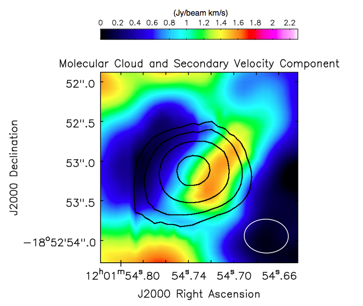
Figure 4.— These observations allow us to disentangle the molecular cloud associated with the secondary velocity component. Contours of the CO(3-2) moment 0 map of the molecular cloud extracted from the 3D data cube (0.4, 0.8, 1.6, 3.2 Jy beam^-1 km s^-1) overlaid on the color moment 0 map of the data cube with the primary cloud extracted. The cloud corresponding to the secondary velocity component can be seen in spatial projection with the primary cloud.

3.2. Cloud Mass

The mass of the cloud is estimated using four different methods, each subject to different caveats. First, given the source size, velocity dispersion of $\sigma_{v}=49\pm 6$ km s^-1, and assuming an isothermal sphere we calculate the virial mass to be in the range of M${}_{vir}=2.9-8.5\times 10^{7}$ M_⊙, which is consistent with the virial mass estimated from ALMA SV observations of $\sim 5\times 10^{7}$ M_⊙ (Herrera et al., 2012). This mass estimate will only be valid if the cloud is in gravitational virial equilibrium; any additional velocity in the cloud will result in this method overestimating the mass. Given the complex dynamical structure of SGMCs, we treat the estimated virial mass as an upper limit.

For the second method we use the RADEX models of the CO(3-2) and CO(2-1) observations to determine the $\chi^{2}$ best fit column density of N${}_{CO}\gtrsim 5\times 10^{18}$ cm^-2. If we assume an abundance ratio of $n_{H2}/n_{CO}=2\times 10^{4}$ (Blake et al., 1987; Wilson & Matteucci, 1992), this column density of CO corresponds to an H₂ mass of M${}_{non-LTE}=2.8\times 10^{6}$ M_⊙. However, the $\chi^{2}$ values are shallow toward higher values of N_CO, and only weakly constrain the upper bound. The models also indicate that the CO(3-2) has an optical depth of $\tau\gtrsim 3$, and therefore this mass estimate is a lower limit.

The third method we employ assumes a conversion factor, X_CO. Values for X_CO in starbursts are known to vary by at least a factor of four (Bolatto et al., 2013), and thus the mass estimated using X_CO should be regarded as uncertain by a corresponding factor. Here we adopt a “starburst” CO-to-H₂ conversion factor X${}_{CO}=0.5\times 10^{20}$ cm^-2(K km s^-1)^-1 (Bolatto et al., 2013). If we were to adopt a “standard” X${}_{CO}=2\times 10^{20}$ cm^-2(K km s^-1)^-1, the resulting cloud mass would be a factor of four larger. We further assume that CO(3-2) is thermalized with respect to CO(1-0) given the brightness temperatures of T${}_{3-2}=17\pm 3$ K and T${}_{2-1}=18\pm 3$ K ; if the lines are not thermalized and CO(3-2) is relatively underpopulated, this mass estimate will be low. This method results in M${}_{X_{CO}}=3.3-15\times 10^{6}$ M_⊙.

The last method estimates the dust mass from the continuum at 870 $\mu$m. The continuum is detected at the 5.4 $\sigma$ level (see Figure 5), with a peak brightness of $9.8\pm 3.4\times 10^{-4}$ Jy beam^-1. Assuming a dust emissivity of $\kappa=0.9\pm 0.13$ cm² g^-1 (Wilson et al., 2008), optically-thin continuum, and a gas-to-dust ratio of 120$\pm 28$, and dust temperature of 20 K (Wilson et al., 2008) this method results in a mass of M${}_{cont}=5\pm 3\times 10^{6}$ M_⊙. Based on the range of mass values determined above, we adopt a cloud mass of M$=0.3-1.5\times 10^{7}$ M_⊙. We note that the virial mass that would be inferred for this cloud appears to be a factor of 5-10$\times$ too high.

Given the estimated mass and size of this cloud, the resulting gas volume density is $\rho\gtrsim 100$ M_⊙ pc^-3. While there are molecular clouds found in the Milky Way with masses of $\sim 10^{6}$ M_⊙, their radii are $~{}2-4\times$ larger, resulting in significantly lower surface densities. Similarly massive clouds have also been identified in other nearby galaxies (Bolatto et al., 2008; Donovan Meyer et al., 2013); their surface densities are also far lower (see Figure 6).

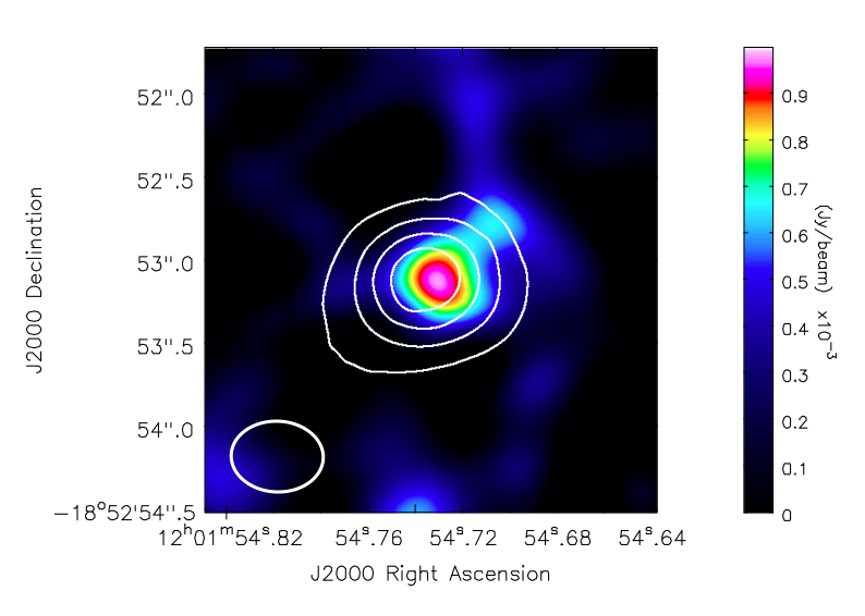
Figure 5.— Detecting the continuum emission associated with this source allows us to determine its dust mass. Contours of the CO(3-2) moment 0 map of the primary cloud overlaid on a color-scale image of the 870 $\mu$m continuum.

We estimate the mass of the stellar cluster that will potentially result from this molecular core by assuming a star formation efficiency (SFE, fraction of mass turned into stars over the lifetime of a cloud). The net efficiency can vary wildly, ranging from a few percent in the Milky Way (e.g. Lada & Lada, 2003), to $>50\%$ in cluster-forming cores by basic boundedness arguments. If we adopt a SFE typical for clusters of $\epsilon=M_{stars}/(M_{stars}+M_{gas})$ of $\sim 20\%-50\%$ (Ashman & Zepf, 2001; Kroupa et al., 2001), an initial cloud mass of $5\times 10^{6}-10^{7}$ M_⊙ would result in a cluster with a mass of $M_{star}=1-5\times 10^{6}$ M_⊙. This would be among the most massive SSCs that have formed in the Antennae if it forms a single cluster (Whitmore et al., 2010). Even if the star formation efficiency were as low as $\sim 5\%$, the resulting cluster would have a mass $>2\times 10^{5}$ M_⊙, still in the regime of super star cluster masses.

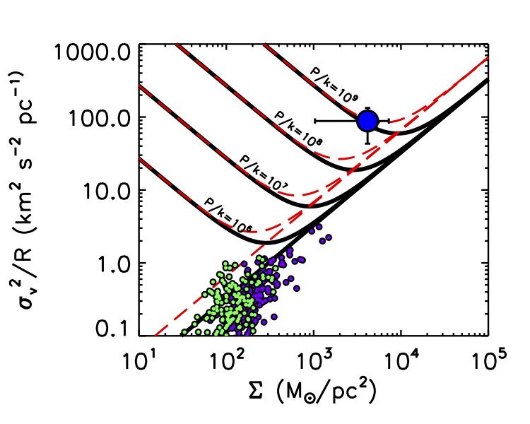
Figure 6.— The measured properties of the primary molecular cloud indicate that it may be subject to pressures of $\sim$P/$k_{B}=10^{9}$ K cm^-3. This plot shows the relationship between surface density and the size-line width coefficient with the candidate proto-super star cluster cloud plotted as the blue point (error bars represent 1$\sigma$). Lines corresponding to pure gravitational virial equilibrium (no external pressure) along with corresponding line for equilibrium with external pressures of P$/k_{B}=10^{6},10^{7},10^{8}$, and $10^{9}$  K cm^-3 are shown in black, corresponding conditions for clouds undergoing free-fall collapse are shown as red dashed lines Field, Blackman, & Keto (2011). For comparison, data points are shown from molecular cloud survey in nearby galaxies as light green points (Donovan Meyer et al., 2013), and Galactic clouds are shown as purple points (Heyer et al., 2009).

3.3. Constraining the Ionizing Flux Associated with the Cloud

In order to assess the extent to which star formation may have already affected the physical state of the ionized gas, we searched for ionizing flux potentially coming from stars within the molecular cloud. Figure 1 shows the Pa$\alpha$ emission in the region, and while there is diffuse emission associated with the SGMC in general, there is no discrete source associated with the molecular cloud in question. However, it is possible that given the embedded nature of this source, Pa$\alpha$ emission could suffer from significant extinction, and thus we also utilize radio observations to identify free-free emission that might be present.

We created two radio maps from archival 3.6 cm VLA observations (proposal codes AN079, AP478, AS796, AA301); one with a synthesized beam of $0.65^{\prime\prime}\times 0.42^{\prime\prime}$ to best match the beam of the ALMA CO(3-2) observations and resolve out diffuse emission, and a second with a synthesized beam of $1.12^{\prime\prime}\times 0.85^{\prime\prime}$, which has greater sensitivity to extended emission. In the higher resolution map, there is no discrete source coincident with the molecular cloud discussed here, and the 5$\sigma$ detection threshold of the radio emission corresponds to an ionizing flux of N${}_{Lyc}\approx 6\times 10^{50}$ s^-1. This is equivalent to $\sim 60$ O-type stars (Vacca et al., 1996). This limit is roughly three times lower than the previous limit placed on possible ionizing flux in this region of $2\times 10^{51}$ s^-1 using lower resolution 6 cm observations (Herrera et al., 2011). For comparison, the ionizing flux of 30 Dor has been estimated to be N${}_{Lyc}\approx 4\times 10^{51}$ s^-1 (Crowther & Dessart, 1998).

In the lower resolution map, while there is no discrete source coincident with the molecular cloud, there is diffuse emission in the region. Without velocity information for this diffuse emission, it is not possible to disentangle potential line-of-sight confusion in this complex region. However, to estimate the possible contribution from stars within this molecular cloud to the diffuse emission, we first fit and subtract Gaussian profiles to the other dominate sources in SGMC2. After subtracting the emission due to nearby sources, we measure the flux density due to diffuse emission in the cloud aperture to be $0.03$ mJy, which corresponds to an ionizing flux of $1.1\times 10^{51}$ s^-1, which corresponds to $\sim 100$ O-type stars (Vacca et al., 1996). However, the diffuse morphology of this emission is not consistent with it coming from a single compact source.

Thus, while both the Pa${\alpha}$ and cm radio observations show diffuse emission associated with the SGMC2 structure, there is no discrete source associated with the compact cloud discussed here (Figure 1). We constrain the possible ionizing flux that could be due to embedded stars in this cloud to be $\lesssim 60$ O-type stars. We can rule out an existing stellar cluster in this molecular core $\gtrsim 10^{4}$ M$\odot$ (Leitherer et al., 1999), roughly two orders of magnitude smaller than the anticipated cluster mass (Section 3.2). Either star formation has not begun or it is so deeply embedded that its ionizing radiation is confined by gas continuing to accrete onto the protostars.

3.4. Determination of Cloud Pressure

With a surface density of $\sim 4\times 10^{3}$ M_⊙ pc^-2 and size-linewidth coefficient of $\sigma^{2}/R=90$ km² s^-2 pc, the cloud is not consistent with being in either pure gravitational virial equilibrium or free-fall collapse (Figure 6, Heyer et al., 2009). Nevertheless, the morphology of the cloud indicates that gravity is playing a significant role (round, compact, and bright – making it stand out as a singular object in the data cube), suggesting that it is not a transient object. As illustrated in Figure 6, the observed line width value can be explained if the cloud is subject to external pressures of P/$k_{B}\sim 10^{9}$ K cm^-3, roughly five orders of magnitude higher than that typical in the interstellar medium of a galaxy (Jenkins et al., 1983). This is consistent with theoretical considerations that have argued SSC formation requires extreme pressures (P/$k_{B}\gtrsim 10^{8}$ K cm^-3) (Jog & Soloman, 1992; Elmegreen & Efremov, 1997; Ashman & Zepf, 2001). This high pressure is also in accord with previous findings of compressive shocks in the overlap region (Wei et al., 2012).

3.5. Expected Proto Super Star Cluster Cloud Size

The expected physical size of a molecular cloud capable of forming an SSC can be estimated based on virial theorem arguments. Following previous work (Elmegreen, 1989), the external cloud pressure $P_{e}$, cloud mass $M$, cloud radius $r$, and velocity dispersion $\sigma_{v}$ can be related by

$P_{e}=\dfrac{3\Pi M\sigma_{v}^{2}}{4\pi r^{3}}$,

where $\Pi$ is defined by $n_{e}=\Pi\langle n_{e}\rangle$, and here we adopt $\Pi=0.5$. It has been estimated that SSC formation requires internal pressures of $P_{0}/k\gtrsim 10^{8}\;$K cm^-3 (Elmegreen & Efremov, 1997). These high pressures inhibit the dispersal of the natal material and achieve sufficiently high star formation efficiencies in the cloud core. If we adopt a minimum mass of $M=10^{6}$ M_⊙ for a cloud capable of forming a SSC, the resulting cloud radius is $r\sim 25$ pc. Likewise, for the velocity dispersion of $\sigma_{v}=49$ km s^-1 observed for the cloud discussed here and the apparent external pressure of $P_{0}/k\gtrsim 10^{9}\;$K cm^-3 (see Figure 6), the expected radius is $r\sim 25$ pc, which is within the uncertainty of the cloud half-light radius of $\lesssim 24\pm 3$ pc extracted from these observations.

4. Discussion

4.1. On the Origin of the High Pressure Inferred for the Molecular Cloud

If the cloud is confined, as we expect from such a strong concentration of gas, then external pressure must play a key role. This high external pressure could result from the weight of the surrounding SGMC2 (if the SGMC is roughly in hydrostatic equilibrium) and/or large scale compressive shocks. The pressure generated by the surrounding molecular material can be estimated using P${}_{G}/k_{B}\approx 1.5$ cm^-3 K (M_cloud/M_⊙)²(r/pc)^-4 (Bertoldi & McKee, 1992). The SGMC2 region has an estimated total mass of $\sim 4\times 10^{8}$ M_⊙ (Wilson et al., 2000) and radius of $\sim 400$ pc, resulting in a pressure from the overlying molecular material of P/$k_{B}\sim 10^{7}$ K cm^-3, which is at least an order of magnitude less than the internal pressure inferred for this cloud.

Given that this cloud is not only in the “overlap” region of the Antennae, but also appears to be at the nexus of two filaments of CO(3-2) emission that are suggestive of colliding flows (Whitmore et al., 2014), a significant amount of external pressure could also be generated by ram pressure. This interpretation is consistent with previous work indicating strong H₂ line emission and an abrupt velocity gradient across this region (Herrera et al., 2011, 2012). However, the morphology of the cloud suggests an isotropic source of pressure, which is in tension with a ram pressure origin.

4.2. Timescales for Cloud Evolution and Star Formation

The relevant timescales for this cloud to evolve are driven by the free-fall time and the crossing time. The compact size and marginally-resolved round morphology suggest that self-gravity has had a significant role in shaping the source, although that is not possible to conclusively demonstrate with the data in hand. The cloud must be largely supported by turbulence: given the inferred density of the cloud (n$\sim 10^{3}$ cm^-3), if the pressure were entirely thermal, it would require a gas temperature of $\sim 10^{5}$ K, which is not reasonable or consistent with these observations that indicate $T\sim 25$ K. We conclude that this cloud is most likely supported by turbulence. This conclusion is also supported by the virial mass being nearly an order of magnitude larger than the mass inferred from the dust continuum, indicating significant internal motion contributing to the observed line width.

Thus, we adopt the turbulent crossing time as the appropriate timescale for the evolution of this cloud and estimate it as $t_{cr}\sim D/\sigma_{V}\sim 1$ Myr, where $D$ is the diameter of the region. If self-gravity is not important, the cloud will disperse on this timescale – the turbulence will dissipate on this timescale in any case. If self-gravity is important (as argued above), the cloud will collapse on this timescale. The free-fall time of the cloud can be estimated as $t_{ff}=(3\pi/32~{}G~{}\rho)^{1/2}\approx 8\times 10^{5}$ years. Given the strong associated H₂ emission (Herrera et al., 2012) and line-width, which indicates internal velocities higher than virial equilibrium, it is plausible that this cloud has already begun free-fall collapse, in which case we are witnessing a very short-lived stage of cluster evolution. Given these arguments, we expect this cloud to collapse on timescales $\lesssim 1$ Myr.

4.3. Expected Number of Proto-SSC Molecular Clouds

Given that this phase of SSC formation is expected to be extremely short-lived ($\lesssim 10^{5}-10^{6}$ yr), it is not surprising that this is the only clear example that we have found to date of a compact cloud without associated star formation that is sufficiently massive to form an SSC. Within $\sim 1$ Myr, we expect that this cloud will be associated with star formation, similar to the clouds observed in M82 by Keto et al. (2005).

The estimated current star formation rate (SFR) for the Antennae is $\sim 7-20$ M_⊙ yr^-1 (Zhang, Fall, & Whitmore, 2001; Brandl et al., 2009). If cluster formation follows a power-law distribution of $dN/dM\propto M^{-2}$ (Zhang & Fall, 1999) with lower and upper masses of $10^{2}$ and $10^{7}$ M_⊙, we expect $\sim 20$% of the stellar mass to be formed in clusters with M$>10^{6}$ M_⊙. Thus we expect only a few SSCs masses of $>10^{6}$ M_⊙ to form every $\sim 5\times 10^{5}$ years. Optical studies indicate that there are six SSCs with ages $<10^{7}$ years and masses $>10^{6}$ M_⊙ (Whitmore et al., 2010). This suggests that a massive cluster is formed every $<$10⁷/6 $\approx$ 1.7$\times$10⁶ years, in agreement with the estimate derived above from the total SFR. The predicted number of pre-stellar molecular clouds capable of forming an SSC with mass $>10^{6}$ M_⊙ can be generalized as,

$$N_{\rm SSC-GMC}\,\simeq\,0.2\times t_{collapse}\left(\frac{\rm SFR{(M_{\odot}yr^{-1})}}{\rm 10^{6}M_{\odot}}\right)$$ (1)

where t_collapse is the timescale for cloud collapse (see Section 4.2). Given a dynamical timescale for this cloud of $\sim 0.5-1$ Myr, we expect that if we observed the Antennae system at any point in its recent star forming history ($\sim 10^{7-8}$ yr), we would find at most one cloud of this evolutionary state and mass.

4.4. Implications for Globular Cluster Formation

The physical properties of this cloud can provide insight into a mode of star formation that may have been dominant in the earlier universe, when globular clusters were formed prolifically. In particular, the pressure of P/$k_{B}\gtrsim 10^{8}$ K cm^-3 supports the hypothesis that such high pressures are necessary to form SSCs (Ashman & Zepf, 2001; Elmegreen, 2002). Based on what appears to be a nearly universal power-law distribution of cluster masses, numerous studies have suggested that the formation of SSCs is statistical in nature, resulting from a “size of sample” – galaxies with higher star formation rates will form more clusters overall, and the formation of SSCs results from populating the tail of the mass distribution (Fall & Chandar, 2012). Based on these ALMA observations, we suggest an alternate interpretation: in a turbulent interstellar medium, the pressure distribution also has a power-law form, and the properties of clusters that form track the pressure distribution. Thus, while galaxies present a power-law distribution of cluster masses, only regions with sufficiently high pressure will be able to form the most massive SSCs. If pressures P/$k_{B}\gtrsim 10^{8}$ K cm^-3 are indeed required to form SSCs (and the surviving globular clusters), similarly high pressures must have been common during the peak of globular cluster formation a few billion years after the Big Bang.

References

- Ashman & Zepf (2001) Ashman, K. M. & Zepf, S. E. AJ, 122, 1888-1895 (2001)
- Aversa et al. (2011) Aversa, A. G., Johnson, K. E., Brogan, C. L., Goss, W. M., & Pisano, D. J. AJ, 141, 125-137 (2011)
- Bastian et al. (2012) Bastian, N., Adamo, A., Gieles, M., Silva-Villa, E. Lamers, H. J. G. L. M., Larson, S. S., Smith, L. J., Konstantopoulos, I. S., & Zackrisson, E. Mon. Not. R. Astron. Soc., 419, 2606-2622 (2012)
- Beck, Turner, & Kovo (2000) Beck, S. C., Turner, J. L., & Kovo, O. 2000, AJ, 120, 244
- Beck et al. (2002) Beck, S. C., Turner, J. L., Langland-Shula, L. E., Meier, D. S., Crosthwaite, L. P., & Gorjian, V. 2002, AJ, 124, 2516
- Beck et al. (2004) Beck, S. C., Garrington, S. T., Turner, J. L. & Van Dyk, S. D. 2004, AJ, 128, 1552
- Bertoldi & McKee (1992) Bertoldi, F. & McKee, C. F. ApJ, 395, 140-157 (1992)
- Blake et al. (1987) Blake, G. A., Sutton, E. C., Masson, C. R., & Phillips, T. G. ApJ, 315, 621-645 (1987)
- Bolatto et al. (2008) Bolatto, A. D., Leroy, A., Rosolowsky, W., Walter, F. & Blitz, L. ApJ, 686, 948-965 (2008)
- Bolatto et al. (2013) Bolatto, A. D., Wolfire, M., & Leroy, A. K. Ann. Rev. Astron. Astrophys, 51, 207-268 (2013)
- Bolte & Hogan (1995) Bolte, M. & Hogan, C. J. Nature, 376, 6539, 399-402 (1995)
- Brandl et al. (2009) Brandl, B. R., Snijders, L., den Brok, M., Whelan, D. G., Groves, B., van der Werf, P., Charmandaris, V., Smith, J. D., Armus, L., Kennicutt, R. C., Jr., Houck, J. R. ApJ, 699, 1982-2001 (2009)
- Brogan et al. (2010) Brogan, C., Johnson, K., & Darling, J. ApJ, 716, 51-56 (2010)
- Carretta et al. (2000) Carretta, E., Gratton, R.G., Clementini, G., & Fusi Pecci, F. ApJ, 533, 215-235 (2000)
- Crocker et al. (2010) Crocker, R. M., Jones, D. I., Melia, F., Ott, J., Protheroe, R. J. 2010, Nature, 463, 7277, 65
- Crowther & Dessart (1998) Crowther, P.A. & Dessart 1998, MNRAS, 296, 622
- Donovan Meyer et al. (2013) Donovan Meyer, D., Koda, J., Momose, R., Mooney, T., Egusa, F., Carty, M., Kennicutt, R., Kuno, N., Rebolledo, D., Sawada, T., Scoville, N., & Wong, T. ApJ, 772, 107-123 (2013)
- Elmegreen (1989) Elmegreen, B. G ApJ, 338, 178-196 (1989)
- Elmegreen & Efremov (1997) Elmegreen, B. G. & Efrefmov, Y. N. ApJ, 480, 235-245 (1997)
- Elmegreen (2002) Elmegreen, B. G. 2002, ApJ, 577, 206
- Espada et al. (2012) Espada, D. et al. ApJ, 760, 25-30 (2012)
- Fall & Zhang (2001) Fall, S. M. & Zhang, Q. Clusters. ApJ, 561, 751-765 (2001)
- Fall et al. (2009) Fall, S. M., Chandar, R., & Whitmore, B. C. ApJ, 704, 453-468 (2009)
- Fall & Chandar (2012) Fall, S. M. & Chandar, R. 2012, ApJ, 752, 96
- Field, Blackman, & Keto (2011) Field, G. B., Blackman, E. G., & Keto, E. R. 2011, MNRAS, 416, 710
- Freedman et al. (1994) Freedman, W. L. et al. ApJ, 427, 628-655 (1994)
- Gnedin & Ostriker (1997) Gnedin, O. Y. & Ostriker, J. P. ApJ, 474, 223-255 (1997)
- Harris et al. (1994) Harris, W. E. & Pudritz, R. E. ApJ, 429, 177-191 (1994)
- Harris et al. (2013) Harris, W. E., Harris, G. L. H., Alessi, M., ApJ, 772, 82-95 (2013)
- Herrera et al. (2011) Herrera, C. N., Boulanger, F., & Nesvadba, N. P. H. Astron. Astrophys, 534, 138-151 (2011)
- Herrera et al. (2012) Herrera C. N., Boulanger, F., Nesvadba, N. P. H., & Falgarone, E. Astron. Astrophys, 538, 9-13 (2012)
- Heyer et al. (2009) Heyer, M., Krawczyk, C., Duval, J., & Jackson, J. M. ApJ, 699, 1092-1103 (2009)
- Jenkins et al. (1983) Jenkins, E. B., Jura, M., & Loewenstein, M. ApJ, 270, 88-104 (1983)
- Jog & Soloman (1992) Jog, C.J. & Soloman, P.M. 1992, ApJ, 387, 152
- Johnson et al. (2001) Johnson, K. E., Kobulnicky, H. A., Massey, P., & Conti, P. S. 2001, ApJ, 559
- Johnson (2002) Johnson, K. E. Science, 297, 5582, 776-777 (2002)
- Johnson et al. (2003) Johnson, K. E. & Kobulnicky, H. A. ApJ, 597, 923-928 (2003)
- Johnson et al. (2004) Johnson, K. E., Indebetouw, R., Watson, C., & Kobulnicky, H. A. AJ, 128, 610-616 (2004)
- Johnson, Hunt, & Reines (2009) Johnson, K. E., Hunt, L. K., & Reines, A. E. 2009, AJ, 137, 3788
- Kepley et al. (2014) Kepley, A. A., Reines, A. E., Johnson, K. E., & Walker, L. M. 2014, AJ, 147, 43
- Keto et al. (2005) Keto, E., Ho, L. C., Lo, K. -Y., ApJ, 635, 1062-1076 (2005)
- Kobulnicky & Johnson (1999) Kobulnicky, H. A. & Johnson, K. E. ApJ, 527, 154-166 (1999)
- Kroupa et al. (2001) Kroupa, P., Aarseth, S., & Hurley, J. MNRAS, 321, 699-712 (2001)
- Lada & Lada (2003) Lada, C. J. & Lada, E. A. 2003, ARAA, 41, 57
- Leitherer et al. (1999) Leitherer, C. et al. ApJS, 123, 3-40 (1999)
- McLaughlin & Fall (2008) McLaughlin, D. E. & Fall, S. M. ApJ, 679, 1272-1287 (2008)
- Mengel et al. (2005) Mengel, S., Lehnert, M. D., Thatte, N., & Genzel, R. A&A, 443, 41-60 (2005)
- Miocchi et al. (2013) Miocchi, P., Lanzoni, B., Dalessandro, E., Vesperini, E., Pasquato, M., Beccari, G., Pallanca, C., & Sanna, N. ApJ, 774, 151-167 (2013)
- O’Connell et al. (1994) O’Connell, R. W., Gallagher, J. S., III, & Hunter, D. A. ApJ, 433, 65-79 (1994)
- Peebles & Dicke (1968) Peebles, P. J. E. & Dicke, R. H. ApJ, 154, 891-908 (1968)
- Reines et al. (2008) Reines, A. E., Johnson, K. E., & Goss, W. M. (2008), ApJ, 685, 39
- Rosolowsky & Leroy (2006) Rosolowsky, R. & Leroy, A. PASP, 118, 590-610 (2006)
- Schweizer, et al. (2008) Schweizer, F. et al. AJ, 136, 1482-1489 (2008)
- Shirley et al. (2013) Shirley, Y. L., Ellsworth-Bowers, T. P., Svoboda, B., Schlingman, W. M., Ginsburg, A., Rosolowsky, E., Gerner, T., Mairs, S., Battersby, C., Stringfellow, G. Dunham, M., Glenn, J., & Bally, J. ApJS, 209, 2-17 (2013)
- Tsai et al. (2009) Tsai, C. -W., Turner, J. L., Beck, S. C., Meier, D. S., Ho, P. T. P. AJ, 137, 4655-4669 (2009)
- Turner et al. (2000) Turner, J. L., Beck, S. C., & Ho, P. T. P. ApJ, 532, 109-112 (2000)
- Turner & Beck (2004) Turner, J. L. & Beck, S. C. ApJ, 602, 85-88 (2004)
- Turner, Ho, & Beck (1998) Turner, J. L., Ho, P. T. P., & Beck, S. C., 1998, 116, 1212
- Ueda et al. (2012) Ueda, J. et al., ApJ, 745, 65-79 (2012)
- Vacca et al. (1996) Vacca, W. D., Garmany, C. D., & Shull, J. M. ApJ, 460, 914-931 (1996)
- van den Bergh et al. (1991) van den Bergh, S., Morbey, C., Pazder, J. ApJ, 375, 594-599 (1991)
- van der Tak et al. (2007) van der Tak, F. F. S., Black, J. H., Schoier, F. L., Jansen, D. J., & van Dishoeck, E. F. Astron. Astrophys, 468, 627-635 (2007)
- Wei et al. (2012) Wei, L. H., Keto, E., Ho, L. C. ApJ, 760, 136-154 (2012)
- Whitmore, Chandar, & Fall (2007) Whitmore, B.C., Chandar, R., & Fall, S.M. 2007, AJ, 133, 1067
- Whitmore et al. (2010) Whitmore, B. C. et al. AJ, 140, 75-109 (2010)
- Whitmore et al. (2014) Whitmore, B. C, Brogan, C., Chandar, R., Evans, A., Hibbard, J., Johnson, K., Leroy, A., Privon, G., Remijan, A., Sheth, K. ApJ (in press)
- Wilson & Matteucci (1992) Wilson, T. L. & Matteucci, F. Astron. Astrophys. Rev., 4, 1-33 (1992)
- Wilson et al. (2000) Wilson, C. D., Scoville, N., Madden, S. C., & Charmandaris, V. ApJ, 542, 120-127 (2000)
- Wilson et al. (2008) Wilson, C. D. et al. ApJS, 178, 189-224 (2008)
- Zhang & Fall (1999) Zhang, Q. & Fall, S. M. ApJ, 527, 81-84 (1999)
- Zhang, Fall, & Whitmore (2001) Zhang, Q., Fall, S.M., Whitmore, B.C. 2001, ApJ, 561, 727