A Parallel Dual Fast Gradient Method for MPC Applications^∗

Abstract

We propose a parallel adaptive constraint-tightening approach to solve a linear model predictive control problem for discrete-time systems, based on inexact numerical optimization algorithms and operator splitting methods. The underlying algorithm first splits the original problem in as many independent subproblems as the length of the prediction horizon. Then, our algorithm computes a solution for these subproblems in parallel by exploiting auxiliary tightened subproblems in order to certify the control law in terms of suboptimality and recursive feasibility, along with closed-loop stability of the controlled system. Compared to prior approaches based on constraint tightening, our algorithm computes the tightening parameter for each subproblem to handle the propagation of errors introduced by the parallelization of the original problem. Our simulations show the computational benefits of the parallelization with positive impacts on performance and numerical conditioning when compared with a recent nonparallel adaptive tightening scheme.

I Introduction

Model Predictive Control (MPC) is a consolidated control technique that can efficiently handle constraints on the process to be controlled. Nevertheless, its application is not yet widespread in many domains where real-time computational constraints and requirements of certified solutions are of major concern, such as aerospace or automotive applications. There is a growing interest in both industry and academia for exploring parallel solutions to MPC problems ([1, 2, 3]), especially in light of the emerging many-core architectures, aiming to improve the computational efficiency of solving the underlying optimization problem.

Contribution. In this paper, we explore the use of parallelization techniques to efficiently solve a typical MPC problem for a linear discrete-time system, with a substantial computational speedup compared to nonparallel implementations. Our proposed algorithm combines the use of Alternating Direction Method of Multipliers (ADMMs [4], [5]) to handle the coupling constraints that arise from the dynamics of the system and inexact solvers (i.e., solvers that guarantee feasibility and optimality only asymptotically with the number of iterations), such as the Nesterov’s Dual Fast Gradient (DFG) method [10]. In particular, the first step of the proposed algorithm is to split the original MPC problem over the length $N$ of the prediction horizon into $N+1$ independent subproblems (time-splitting [3]) solved by $N+1$ parallel workers periodically exchanging information at predetermined synchronization points. Then, the second step is to solve these subproblems in parallel using an inexact solver and guarantee, at the same time, that the solution of the original MPC problem is recursively feasible and the system is closed-loop stable. The combination of parallelization and inexact solvers can result in infeasibility and closed-loop instability. We rely on an algorithm based on constraint tightening to overcome these issues. Loosely speaking, constraint-tightening algorithms solve an alternative problem in which the constraints have been tightened by a certain amount to compensate for the accuracy loss (and possible related infeasibility) introduced by the solver. We rely on an adaptive tightening strategy to select an appropriate amount of tightening for our algorithm. Every time new measurements are available from the plant, our algorithm chooses the amount of tightening required for each subproblem in order to compensate for the error introduced by the time-splitting combined with the inexact solver.

Related work. The time-splitting technique has been proposed in [3]. In contrast to [3], we combine ADMM with inexact solvers and focus on the requirements for recursive feasibility and closed-loop stability of the original problem.

Other constraint-tightening schemes have been proposed in the literature (outside the parallel framework). For example, the authors in [7] propose an algorithm in which the amount of tightening is chosen offline to guarantee suboptimality and feasibility of the solution for all the initial states of the MPC problem. Solutions based on adaptive constraint tightening have been recently proposed in [8], where the tightening parameter is chosen adaptively. Compared to [8], our tightening update rule allows for a nonuniform amount of tightening (the tightening varies along the prediction horizon). Furthermore, thanks to the modular structure of our approach, the optimizer solves simpler problems of fixed dimension, which is independent from $N$. As a consequence, an increase of $N$ does not affect the conditioning of the problem and the convergence of the solver. Hence, our approach leads to a performance improvement even when forcing full serialization of the parallel operations (i.e., serialized mode [9]).

Outline. In the following, Section II presents the initial problem formulation. Section III introduces the auxiliary subproblems and our proposed solver. Section IV describes our strategy to select the tightening of each subproblem to handle the parallelization error. Section V proposes an online update strategy of the tightening parameters that guarantees recursive feasibility, suboptimality, and closed-loop stability. Section VI presents numerical results using an academic example. Finally, Section VII concludes the paper.

Notation. For $u\in\mathbb{R}^{n}$, $\left\|u\right\|=\sqrt{\langle u,u\rangle}$ is the Euclidean norm and $\left[u\right]_{+}$ is the projection onto non-negative orthant $\mathbb{R}^{n}_{+}$. Given a matrix $A$, $[A]_{i}$ denotes the $i$-th row of A and $[A]_{i,j}$ the entry $(i,j)$ of A. Furthermore, $\mathbf{1}_{n}$ is the vector of ones in $\mathbb{R}^{n}$ and $I_{n}$ the identity matrix in $\mathbb{R}^{n\times n}$. In addition, $\textrm{eig}_{\max}(A)$ and $\textrm{eig}_{\min}(A)$ denote the largest and the smallest (modulus) eigenvalues of the matrix A, respectively. $P\in\mathbb{S}^{{n}}_{>0}$ denotes that $P\in\mathbb{R}^{n\times n}$ is positive definite.

II Problem Formulation

Consider the discrete-time linear system described below:

$$x(t+1)=Ax(t)+Bu(t)\quad\quad\forall t\geq 0,$$ (1)

where $x(t)\in\mathcal{X}\subseteq\mathbb{R}^{n}$ denotes the state of the system and $u(t)\in\mathcal{U}\subseteq\mathbb{R}^{m}$ denotes the control input. The sets $\mathcal{X}$ and $\mathcal{U}$ are simple proper convex sets (i.e., convex sets that contain the origin in their interior). Our goal is to steer $x(t)$ to the origin and satisfy the plant constraints. We use MPC to achieve these objectives. In this respect, consider the following finite-time optimal control problem:

$$\mathcal{V}^{*}(x_{\textrm{init}})= {\underset{x,u}{\text{min}}}~{}\frac{1}{2}\sum\limits_{t=0}^{N-1}(x_{t}^{T}Qx_{t}\!+\!u_{t}^{T}Ru_{t})+x_{N}^{T}P_{N}x_{N}$$ (2a)

s.t.: $$x_{t+1}=Ax_{t}+Bu_{t},\quad~{}~{}t\!=\!0,\ldots,N-1$$ (2b)

$$Cx_{t}+Du_{t}+g\leq 0,~{}t\!=\!0,\ldots,N-1$$ (2c)

$$x_{0}=x_{\textrm{init}}$$ (2d)

$$x_{N}\in\mathcal{X}_{N}.$$ (2e)

where $x_{t}$ and $u_{t}$ are more compact notations for $x(t)$ and $u(t)$, respectively. For $t\!=\!0,\ldots,N-1$ ($N$ denotes the prediction horizon), the states and the control inputs are constrained in the polyhedral set described by (2c), where $C\in\mathbb{R}^{p_{t}\times n}$, $D\in\mathbb{R}^{p_{t}\times m}$, $g\in\mathbb{R}^{p_{t}}$. Note that (2c) can include constraints on the state only, i.e., $x_{t}\in\mathcal{X}$, and/or constraints on the control inputs only, i.e., $u_{t}\in\mathcal{U}$. In (2a), $Q\in\mathbb{S}^{{n}}_{\geq 0}$ and $R\in\mathbb{S}^{{m}}_{>0}$. Our problem formulation considers also a terminal cost $x_{N}^{T}P_{N}x_{N}$ associated with a terminal polyhedral set $\mathcal{X}_{N}~{}:=~{}\{x\in\mathbb{R}^{n}|F_{N}x\mathbf{\leq}f_{N},F_{N}\in\mathbb{R}^{p_{N}\times n},f_{n}\in\mathbb{R}^{p_{N}}\}$.

Through the remaining of the paper, we assume:

Assumption 1.

The pair $(A,B)$ is stabilizable.

Assumption 2.

Suppose Assumption 1 holds. Given the gain $K_{f}\in\mathbb{R}^{m\times n}$ obtained by the infinite-horizon linear quadratic regulator (IH-LQR)—characterized by the matrices $A$, $B$, $Q$, and $R$—the following holds:

$$\forall x\in\mathcal{X}_{N}~{}\Rightarrow~{} \begin{cases}x\in\mathcal{X},~{}K_{f}u\in\mathcal{U},~{}\text{and}\\ (A+BK_{f})x\in\mu\mathcal{X}_{N},~{}0\leq\mu<1.\end{cases}$$

In addition, the terminal penalty $P_{N}\in\mathbb{S}^{{n}}_{>0}$ in the stage cost (2a) is defined by the solution of the algebraic Riccati equation associated with the IH-LQR.

In general, the MPC controller solves the optimization problem (2) every time new measurements are available from the plant and returns an optimal sequence of states and control inputs that minimizes the cost (2a). Let the optimal sequence be defined as follows:

$$\{\mathbf{x},\mathbf{u}\}:=\{x_{0},\ldots,x^{*}_{N},u_{0}^{*},\ldots,u_{N-1}^{*}\}.$$ (3)

Only the first element of $\mathbf{u}$ is implemented in closed-loop, i.e., the control law obtained using the MPC controller is given by:

$$\kappa_{\text{MPC}}(x_{\text{init}})=u_{0}^{*},$$ (4)

and the closed-loop system is described by

$$x(t+1)=Ax(t)+B\kappa_{\text{MPC}}(x_{\text{init}}).$$ (5)

II-A Parallelization

We aim to solve Problem (2) in parallel. Hence, we exploit a similar approach as the one proposed in [3]. Specifically, as in [3], Problem (2) is decomposed along the length of the prediction horizon $N$ into $N+1$ independent subproblems to be solved by $N+1$ parallel workers $\Pi_{t}$ ($t\!=\!0,\ldots,N$). Each $\Pi_{t}$ is allowed to communicate with its neighbours $\Pi_{t-1}$ and $\Pi_{t+1}$ at predefined synchronization points. The decomposition is possible thanks to the introduction of $N$ auxiliary variables $z_{t}~{}(t\!=\!1,\ldots,N)$ used to break the dynamic coupling that arises from (2b). These $z_{t}$ can be seen as the global variables of the algorithm. In particular, each $z_{t}$ stores the local predicted state $x_{t+1}$ of each subproblem and exchanges this stored information to guarantee consensus between neighboring subproblems, i.e., to ensure that the predicted state of the $(t)$-th subproblem, namely $x_{t+1}^{(t)}$, is equal to the current state of the $(t\!+\!1)$-st subproblem, namely $x_{t+1}^{(t+1)}$. Specifically, by introducing the consensus constraints $z_{t+1}\!=\!x_{t+1}^{(t)}\!=\!x_{t+1}^{(t+1)}$, defining $y_{t}:=[x_{t}^{(t)T}~{}u_{t}^{(t)T}]^{T}$, $H_{1}:=[I_{n}~{}0]$, $H_{2}:=[A~{}B]$, $\rho>0$ Problem (2) becomes:

$${\underset{y,z}{\text{min}}}~{}\sum\limits_{t=0}^{N}\mathbf{V}_{t}\big{(}y_{t},z_{t}\big{)}$$ (6a)

$$\text{s.t.: }G_{t}y_{t}+g_{t}\leq\!0,\quad~{}t\!=\!0,\ldots,N-1$$ (6b)

$$~{}~{}~{}~{}~{}~{}H_{1}y_{0}=x_{\textrm{init}},$$ (6c)

$$~{}~{}~{}~{}~{}~{}H_{1}y_{N}\in\mathcal{X}_{N},$$ (6d)

$$~{}~{}~{}~{}~{}~{}z_{t+1}=H_{2}y_{t},\quad~{}t\!=\!0,\ldots,N-1,$$ (6e)

$$~{}~{}~{}~{}~{}~{}z_{t+1}=H_{1}y_{t+1},~{}t\!=\!0,\ldots,N-1,$$ (6f)

where, defining $\xi_{t}:=[y_{t}^{T}z_{t}^{T}z_{t+1}^{T}]^{T}$:

• $\mathbf{V}_{0}(\xi_{0}):=\frac{1}{2}\xi_{0}^{T}\mathcal{Q}_{0}\xi_{0}$, where

  $$Q_{0}:=\begin{bmatrix}\mathcal{H}_{0}+\frac{\rho}{2}H_{2}^{T}H_{2}&\frac{\rho}{2}H_{2}\\ -\frac{\rho}{2}H_{2}&\rho I_{n}\end{bmatrix}$$

  and $H_{0}:=\text{diag}\{Q,R\}$.

• $\mathbf{V}_{t}(\xi_{t}):=\frac{1}{2}\xi_{t}^{T}\mathcal{Q}_{t}\xi_{t}$, where, for $t=1,\ldots,N-1$,

  $$Q_{t}:=\begin{bmatrix}\mathcal{H}_{0}+\frac{\rho}{2}(H_{2}^{T}H_{2}+H_{1}^{T}H_{1})&\frac{\rho}{2}H_{1}&\frac{\rho}{2}H_{2}\\ -\frac{\rho}{2}H_{1}&\rho I_{n}&0\\ -\frac{\rho}{2}H_{2}&0&\rho I_{n}\end{bmatrix}$$

• $\mathbf{V}_{N}(\xi_{N}):=\frac{1}{2}\xi_{N}^{T}\mathcal{Q}_{N}\xi_{N}$ where

  $$Q_{N}:=\begin{bmatrix}\mathcal{H}_{N}+\frac{\rho}{2}H_{1}^{T}H_{1}&\frac{\rho}{2}H_{1}\\ -\frac{\rho}{2}H_{1}&\rho I_{n}\end{bmatrix}$$

  and $H_{N}:=\text{diag}\{P_{N},0_{m\times m}\}$.

Furthermore, $G_{t}$ and $g_{t}$ vary for each subproblem as follows:

• $G_{t}:=[C~{}D]$ and $g_{t}:=g$, $t=0,\ldots,N-1$.

• $G_{N}:=[F_{N}~{}0_{p_{N}\times m}]$ and $g_{N}:=-f_{N}$.

Remark 1.

Note that we introduced a quadratic penalty in the cost of the form $\rho/2(\|H_{1}y_{t}-z_{t}\|^{2}+\|H_{2}y_{t}-z_{t+1}\|^{2})$, according to the ADMM strategy [4]. This penalty has no impact on the cost of the original problem (2), if the consensus constraints are satisfied.

In the following, we introduce the subproblems that derive from Problem (6). Let $v_{t+1}$ ($t\!=\!0,\ldots,N-1$) and $w_{t}$ ($t\!=\!1,\ldots,N$) be the Lagrange multipliers associated with the equality constraints (6e) and (6f), respectively. Then, let the augmented Lagrangian with respect to the multipliers $v_{t+1}$ and $w_{t}$ be defined as follows:

$$\mathcal{L}_{v_{t+1},w_{t}}\!\!:= \mathbf{V}_{t}(\xi_{t})\!+\!\rho[v_{t+1}^{T}(H_{2}y_{t}\!-\!z_{t+1})+w_{t}^{T}(H_{1}y_{t}\!-\!z_{t})].$$

Hence, we obtain the following $N+1$ independent subproblems, called original subproblems, associated with the $N+1$ workers $\Pi_{t}$ ($t\!=\!0,\ldots,N$):

$${\underset{y_{t},z_{t}}{\text{min}}}~{}\mathcal{L}_{v_{t+1},w_{t}}(y_{t},z_{t},z_{t+1})~{}\text{s.t.: }G_{t}y_{t}+g_{t}\leq 0.$$ (7)

II-B Overview of our proposed approach and terminology

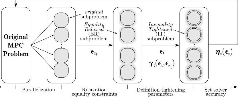
Figure 1: Notation and terminology.

Figure 1 summarizes the main steps that lead to a suboptimal solution of the aforementioned problem and introduces the keywords used in the remaining of the paper. Consider the MPC problem (2) and refer to this problem as the original MPC problem. The first step (parallelization, detailed in Section II-A) is to rewrite the original problem in $N+1$ independent subproblems (the original subproblems). The aim is to use a Dual Fast Gradient (DFG) method to solve these subproblems in order to certify—in terms of suboptimality and recursive primal feasibility, along with closed-loop stability—the MPC solution. The use of the inexact solver will eventually cause a violation of the consensus constraints (6e)-(6f) introduced to define the subproblems (7). Hence, the second step (relaxation equality constraints detailed in Section III-A) is introduced to relax the consensus constraints by a quantity $\epsilon_{z_{t}}$, preventing the occurrence of consensus-constraint violations. We refer to these subproblems as the equality relaxed (ER) subproblems. The set of inequality constraints of the ER subproblems includes the inequality constraints of the original subproblems (7) and the inequality constraints due to the relaxation of the consensus constraints (6e)-(6f). The third step (definition tightening parameters detailed in Sections III-C, IV, and V) is required to address the following remaining issues. First, the solution of each ER subproblem computed by the dual fast gradient method might violate the inequality constraints, due to the termination of the solver after a finite number of iterations. Hence, the constraints of the ER subproblems must be tightened by a quantity $\epsilon_{t}$ proportional to the desired level of suboptimality $\eta_{t}$ chosen by the algorithm. Second, due to the relaxation of the consensus constraints, the consolidated prediction, i.e., the predicted evolution of the state computed (a posteriori) using the control sequence obtained by the independent subproblems, might deviate from the predicted local solution computed by the independent subproblems and, eventually, violate the inequality constraints of the original problem. Hence, an additional tightening (dependent on $\epsilon_{z_{t}}$) must be introduced on the subset of inequality constraints of the ER subproblems that corresponds to the original inequality constraints. The proposed algorithm addresses the aforementioned issues by exploiting the inequality tightened (IT) subproblems. The IT subproblems differ from the ER subproblems in the definition of the feasibility region, which is tightened by a quantity $\gamma_{t}(\epsilon_{t},\epsilon_{z_{t}})$ that depends on both $\epsilon_{t}$ and $\epsilon_{z_{t}}$. The last step (set solver accuracy) selects a suboptimality level $\eta_{t}$ for each subproblem, that guarantees a primal feasible and suboptimal solution for the original MPC problem within a fixed number of iterations.

III Subproblem reformulation

In the following, we introduce the ER subproblems and the proposed algorithm to solve them using $N+1$ parallel workers. Furthermore, we introduce an initial formulation of the IT subproblems and derive conditions on the choice of the relaxation and tightening parameters to guarantee primal feasible and suboptimal solutions for of each subproblem.

III-A Equality constraint relaxation

Our goal is to obtain a solution for Problem (6) by solving the independent subproblems (7) in parallel using inexact solvers, such as the Nesterov’s DFG [10]. In order to use our proposed solver (introduced in Section 1), which relies on first-order methods, we introduce a reformulation of Problem (6) to take into account that the constraints (6e) and (6f) cannot be satisfied at the equality due to the iterative nature of the proposed solver and its asymptotic convergence properties. In particular, introducing the relaxation parameters $\epsilon_{z_{t}},\!\epsilon_{z_{t+1}}\!\!>\!\!0$, for each subproblem ($t\!=\!0,\ldots,N-1$), the former equality constraints (6e)-(6f) are replaced by the following inequality constraints:

$$|H_{1}y_{t}-z_{t}|\leq\epsilon_{z_{t}}\operatorname{\mathbf{1}}_{n} \Leftrightarrow|x_{t}^{(t)}-z_{t}|\leq\epsilon_{z_{t}}\operatorname{\mathbf{1}}_{n},$$ (8a)

$$|H_{2}y_{t}\!-\!z_{t+1}|\!\leq\!\epsilon_{z_{t+1}}\operatorname{\mathbf{1}}_{n} \Leftrightarrow|x_{t+1}^{(t)}\!-\!z_{t+1}|\leq\epsilon_{z_{t+1}}\operatorname{\mathbf{1}}_{n}.$$ (8b)

Thus, for each subproblem, we can realistically consider a feasible region defined by the following constraints:

$$[~{}G_{t}~{}~{}~{}~{}0~{}~{}~{}~{}~{}~{}0]~{}\xi_{t}+~{}g_{t}~{}~{}~{}~{}~{}~{}\leq 0,$$ (9a)

$$[~{}H_{1}~{}-I_{n}~{}~{}~{}~{}0]~{}~{}\xi_{t}-\epsilon_{z_{t}}\mathbf{1}_{n}~{}~{}\leq 0,$$ (9b)

$$[-H_{1}~{}~{}~{}I_{n}~{}~{}~{}~{}0]~{}~{}\xi_{t}-\epsilon_{z_{t}}\mathbf{1}_{n}~{}~{}\leq 0,$$ (9c)

$$[~{}H_{2}~{}~{}~{}~{}0~{}-I_{n}]~{}~{}\xi_{t}-\epsilon_{z_{t+1}}\mathbf{1}_{{n}}\leq 0,$$ (9d)

$$[-H_{2}~{}~{}~{}0~{}~{}~{}~{}I_{n}]~{}\xi_{t}-\epsilon_{z_{t+1}}\mathbf{1}_{{n}}~{}\leq 0,$$ (9e)

or, in a more compact notation:

$$G_{\xi_{t}}\xi_{t}+g_{\xi_{t}}\leq 0,$$ (10)

where $G_{\xi_{t}}\in\mathbb{R}^{p_{\xi_{t}}\times(n+m)+2n}$ and $p_{\xi_{t}}:=p_{t}+4n$.

In the remaining of the paper, we consider the following equality relaxed (ER) subproblems:

$$\mathbf{V}_{t}^{*}={\underset{\xi_{t}}{\text{min}}}~{}\mathbf{V}_{t}(\xi_{t})~{}\text{s.t.:}~{}G_{\xi_{t}}\xi_{t}+g_{\xi_{t}}\!\leq\!0,~{}t\!=\!0,\ldots,N.\vspace{-1cm}$$ (11)

Hence, let $\mu_{t}:=[\lambda_{t}^{T}~{}{w_{t}^{+}}^{T}~{}{w_{t}^{-}}^{T}~{}{v_{t+1}^{+}}^{T}~{}{v_{t+1}^{-}}^{T}]^{T}\in\mathbb{R}^{p_{\xi_{t}}}_{+}$ be the Lagrange multiplier associated with the new set of inequality constraints defined by (10), where $\lambda_{t}$, ${w_{t}^{+}}$ ${w_{t}^{-}}$, ${v_{t+1}^{+}}$, and ${v_{t+1}^{-}}$ are the multipliers associated with the constraints (9a),  (9b),  (9c),  (9d), and (9e), respectively. Then, to handle the complicated constraints (10), define, for each subproblem, the dual function $d_{t}(\xi_{t},\mu_{t})$ as follows:

$$d_{t}(\xi_{t},\mu_{t})={\underset{\xi_{t}}{\text{min}}}~{}\mathcal{L}_{\mu_{t}}(\xi_{t}),$$ (12)

where $\mathcal{L}_{\mu_{t}}(\xi_{t}):=\mathbf{V}_{t}(\xi_{t})+\mu^{T}_{t}\text{diag}\{I_{p_{t}},\rho I_{4n}\}(G_{\xi_{t}}\xi_{t}+g_{\xi_{t}})$. We refer to (12) as the inner subproblem. Hence, we aim to solve the following dual subproblems (outer subproblem) in parallel to obtain a solution for Problem (6):

$$d_{t}^{*}={\underset{\mu_{t}}{\text{max}}}~{}{d}_{t}(\xi_{t},\mu_{t}),~{}t\!=\!0,\ldots,N.$$ (13)

Remark 2.

The size of the ER subproblems remains unaffected if $N$ increases. Intuitively, this modularity is an additional feature that can be exploited to preserve some favorable numerical properties of the problem (e.g., conditioning, Lipschitz constant, etc.) even when the algorithm is running in serialized mode.

III-B Parallel dual fast gradient method

This section introduces Algorithm 1 that we use to solve the MPC problem (6) exploiting $N+1$ parallel workers $\Pi_{t}$. Note that, at this stage, we cannot yet ensure that the computed solution is feasible and suboptimal for Problem (2).

Algorithm 1 relies on Nesterov’s DFG in which the inner problem is solved in an ADMM fashion, as explained below. Specifically, as Figure 2 depicts, at each iteration of the algorithm, $\Pi_{t}$ computes a minimizer $\xi_{t}^{k}$ for $\mathcal{L}_{\mu_{t}}(\xi_{t})$ (steps 1-4), i.e., the algorithm returns a solution for each inner subproblem (12). In particular, our algorithm, in compliance with the ADMM strategy, first minimizes $\mathcal{L}_{\mu_{t}}$ with respect to $y_{t}$ in parallel for each subproblem (step 1). Then, using the information received by $\Pi_{t+1}$, i.e., the updated value of $y^{k+1}_{t+1}$ (synchronization step 2), our algorithm computes—in parallel for each subproblem—the value of the global variable $z_{t}$ according to the following rule (step 3):

$$z_{t}^{k+1}\!=\!\frac{1}{2}({H_{1}y_{t}^{k+1}\!+\!H_{2}y_{t-1}^{k+1}\!+\!v_{t}^{+}\!+\!w_{t}^{+}\!-\!v_{t}^{-}\!-\!w_{t}^{-}}).$$ (14)

Note that this strategy allows to handle the coupling introduced by the 2-norm in the cost function of (11). Then, (synchronization step 4) $\Pi_{t}$ receives (sends) the updated value of $z_{t+1}^{k+1}$ ($z_{t}^{k+1}$) from $\Pi_{t+1}$ (to $\Pi_{t-1}$), respectively. Finally, the worker $\Pi_{t}$ computes the new values of the multipliers $\mu_{t}^{k+1}$ (steps 5-7). We compute offline (for each subproblem) the Lipschitz constant $L_{\mu_{t}}$ associated with $\nabla_{\mu_{t}}d_{t}(\xi_{t},\mu_{t})$ to perform the multipliers’ update:

• $L_{\mu_{0}}=\text{diag}\bigg{\{}\frac{\|G_{0}\|^{2}_{2}}{\textrm{eig}_{\textrm{min}}(\mathbf{Q}_{0})}I_{p_{0}},\frac{\|\rho\text{diag}\{H_{2},-I\}\|^{2}_{2}}{\textrm{eig}_{\textrm{min}}(\mathbf{Q}_{0})}I_{2n}\bigg{\}}$.

• $L_{\mu_{t}}=\text{diag}\bigg{\{}\frac{\|G_{t}\|^{2}_{2}}{\textrm{eig}_{\textrm{min}}(\mathbf{Q}_{t})}I_{p_{t}},\frac{\|\rho\text{diag}\{H_{1},-I\}\|^{2}_{2}}{\textrm{eig}_{\textrm{min}}(\mathbf{Q}_{t})}I_{2n},\\ \frac{\|\rho\text{diag}\{H_{2},-I\}\|^{2}_{2}}{\textrm{eig}_{\textrm{min}}(\mathbf{Q}_{t})}I_{2n}\bigg{\}}$, ($t=1,\ldots,N-1$).

• $L_{\mu_{N}}=\text{diag}\bigg{\{}\frac{\|G_{N}\|^{2}_{2}}{\textrm{eig}_{\textrm{min}}(\mathbf{Q}_{N})}I_{p_{N}},\frac{\|\rho\text{diag}\{H_{1},-I\}\|^{2}_{2}}{\textrm{eig}_{\textrm{min}}(\mathbf{Q}_{N})}I_{2n}\bigg{\}}$.

Given $\xi_{t}^{0},\mu_{t}^{0},Q_{t},G_{t},g_{t},L_{\mu_{t}}$, and $\bar{k}_{t}$ for each $\Pi_{t}$ ($t\!=\!0,\ldots,N$)

while $k\leq\bar{k}_{t}$ do

     1. $\Pi_{t}$ computes $y_{t}^{k+1}\!=\!\operatorname{argmin}_{y_{t}}~{}\mathcal{L}_{\mu_{t}}(\xi_{t}^{k},\mu_{t}^{k}).$

     2. $\Pi_{t}$ receives $y_{t+1}^{k+1}$ from $\Pi_{t+1}$, send $y_{t}^{k+1}$ to $\Pi_{t-1}$.

     3. $\Pi_{t}$ updates $z_{t}^{k+1}$ according to (14).

     4. $\Pi_{t}$ receives $z_{t+1}^{k+1}$ from $\Pi_{t+1}$, sends $z_{t}^{k+1}$ to $\Pi_{t-1}$.

     5. $\Pi_{t}$ computes

$$\hat{\mu}_{t}^{k+1}=\bigg{[}\mu^{k}_{t}+L_{\mu_{t}}^{-1}\nabla^{T}_{\mu_{t}}d_{t}(\xi_{t}^{k+1},\mu_{t})\bigg{]}_{+}.$$

     6. Define: $a:=\!\frac{k+1}{k+3}I$, $b_{\mu_{t}}\!:=\!\!L_{\mu_{t}}^{-1}\frac{2}{(k+3)}$.

     7. $\Pi_{t}$ computes:

$$\mu_{t}^{k+1}\!=\!a\hat{\mu}_{t}^{k+1}\!+\!b_{\mu_{t}}\bigg{[}\!\sum_{s=0}^{k}\frac{s+1}{2}\nabla^{T}_{\mu_{t}}d_{t}(\xi_{t}^{s},\mu_{t})\bigg{]}_{+}.$$

end while

Algorithm 1 Parallel Dual Fast Gradient Method.

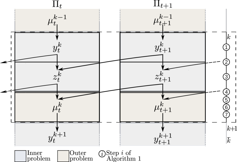
Figure 2: Iteration $k$ of Algorithm 1.

Note that our update rule is different from the one proposed in [6], where ADMM is used in combination with Nesterov’s fast gradient methods. At each iteration, the algorithm proposed in [6], first computes the exact minimizer $y_{t}$ and then updates $v_{t}$ and $w_{t}$. Our algorithm does not wait until the DFG returns a minimizer $y_{t}$ to update the multipliers $v_{t}$ and $w_{t}$, but starts updating their values along with the DFG iterations, encouraging the information exchange between neighboring subproblems. This algorithm is also different from the one proposed in [3]. In particular, the workers exchange the necessary pieces of information before the update of the Lagrange multipliers and none of the dual variables is exchanged between the neighboring workers, as Figure 2 highlights. Furthermore, the information exchange between neighboring workers is unidirectional, i.e., $\Pi_{t+1}$ sends the updated information to $\Pi_{t}$, but $\Pi_{t}$ does not send any updated information to $\Pi_{t+1}$.

Using an argument similar to the one of Theorem 1 in [8], we can compute the primal feasibility violation and the level of suboptimality of the solution of each ER subproblem returned by Algorithm 1.

Theorem 1.

([8]) Let $\mathbf{V}_{t}(\xi_{t})$ be strongly convex, the sequences ($\boldsymbol{\xi}_{t}^{k}$, $\hat{\mu}_{t}^{k}$, $\mu_{t}^{k}$) be generated by Algorithm 1, and $\boldsymbol{\hat{\xi}}_{t}^{k}:=\sum_{s=0}^{k}\frac{2(s+1)}{(k+1)(k+2)}\boldsymbol{\xi}^{s}$. Then, an estimate on the primal feasibility violation for the ER subproblem (11) is given by the following:

$$\|[\nabla_{\mu_{t}}^{T}d_{t}(\boldsymbol{\hat{\xi}}_{t}^{k})]_{+}\|\leq\frac{8R_{t}{\max\{L_{\mu_{t}}\}}}{(k+1)^{2}}=:\eta_{t},$$ (15)

where $R_{t}:=\|\mu^{*}_{t}\|$ . Moreover, an estimate on primal suboptimality is given by the following:

$$0\leq\mathbf{V}_{t}^{*}-\mathbf{V}_{t}(\boldsymbol{\hat{\xi}}_{t})\leq R_{t}\eta_{t}.$$ (16)

Algorithm 1 terminates after a fixed number of iterations that depends on $\eta_{t}$ and $R_{t}$ [8]:

$$\bar{k}_{t}:=\bigg{\lfloor}\sqrt{{8R_{t}\eta_{t}^{-1}{\max\{L_{\mu_{t}}\}}}}\bigg{\rfloor}.$$ (17)

III-C Tightening of the original inequality constraints

In order to guarantee the primal feasibility of each subproblem using Algorithm 1, we introduce $N+1$ auxiliary subproblems, namely the inequality tightened (IT) subproblems, which differ from the ER subproblems (11) in the definition of the feasible region. In particular, each IT subproblem can be defined as follows:

$$\mathbf{V}_{\epsilon_{t}}^{*}\!=\!\min_{\xi_{t}}\mathbf{V}_{t}(\xi_{t})~{}\text{s.t.:}~{}G_{\xi_{t}}\xi_{t}+g_{\xi_{t}}+\mathbf{\epsilon}_{t}\mathbf{1}_{p_{t}+4n}\leq 0,$$ (18)

where $\epsilon_{t}\geq 0$ is the tightening parameter, which depends on the suboptimality level $\eta_{t}$ that the proposed algorithm can reach within $\bar{k}_{t}$ iterations (17). According to [8], solving (18) using Algorithm 1 ensures, with a proper choice of $\epsilon_{t}$, that the solution of (18) is primal feasible and suboptimal for subproblem (11).

To define an $\epsilon_{t}$ similar to the one introduced in [8], we must compute an upper bound for the optimal Lagrange multiplier, namely $\mu^{*}_{t,\epsilon_{t}}$, associated with the IT subproblem (18). We use an argument similar to the one of Lemma 1 in [12]. In particular, we compute the aforementioned upper bound for $\mu^{*}_{t,\epsilon_{t}}$ according to the following lemma.

Lemma 1.

Assume that there exists a Slater vector $\tilde{y}_{t}\in\mathbb{R}^{n+m}$ such that $G_{t}\tilde{y}_{t}+g_{t}<0$. Then, there exists $\epsilon_{t}\geq 0$, $\epsilon_{t}<{\min}_{j=1,\ldots,p_{t}}\{-(G_{t}\tilde{y}_{t}+g_{t})_{j}\}$, $\epsilon_{z_{t}},\epsilon_{z_{t+1}}>\epsilon_{t}$, such that the upper bound for $\mu^{*}_{t,\epsilon_{t}}$ is given by

$$\|\mu_{t,\epsilon_{t}}^{*}\|\leq 2{R_{d_{t}}}:=2{\frac{\mathbf{V}_{t}(\tilde{\xi}_{t})-d_{t}(\tilde{\mu}_{t})}{\min\limits_{j=1,\ldots,p_{t}+2n}\{[\Gamma_{t}]_{j}\}}},$$ (19)

where $\Gamma_{t}\!\!:=\!\!\!\big{[}[-(G_{t}\tilde{y}_{t}\!+\!g_{t})^{T}\!-\!\epsilon_{t}\operatorname{\mathbf{1}}_{p_{t}}^{T}][2\rho(\epsilon_{z_{t}}-\epsilon_{t})\operatorname{\mathbf{1}}_{n}^{T}][2\rho(\epsilon_{z_{t+1}}-\epsilon_{t})\operatorname{\mathbf{1}}_{n}^{T}]\big{]}^{T}\in\mathbb{R}^{p_{t}+2n}$, and $d_{t}(\tilde{\mu}_{t})$ is the dual function for the original subproblem (13) evaluated at $\tilde{\mu}_{t}\in\mathbb{R}^{p_{t}+4n}$.

See Appendix A.

Remark 3.

Lemma 1 does not only provide an upper bound for $\|\mu_{t,\epsilon_{t}}^{*}\|$, but it also provides guidelines to select the values of $\epsilon_{z_{t}}$ and $\epsilon_{z_{t+1}}$ as a function of ${\min}_{j=1,\ldots,p_{t}}\{-(G_{t}\tilde{y}_{t}+g_{t})_{j}\}$, which only depends on the primal variable $\tilde{y}_{t}$. An alternative way to determine the relaxation parameters is to include $\epsilon_{z_{t}}$ and $\epsilon_{z_{t+1}}$ in the set of decision variables and penalize them in the cost function as it is usually done to handle soft constraints. This will, however, increase the number of decision variables in the problem formulation and it will have an impact on the original cost.

IV Tightening improvement to guarantee primal feasible consolidated predictions

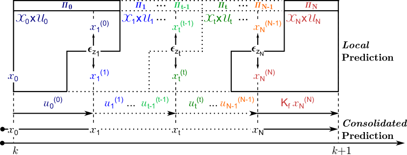
Figure 3: Local and consolidated  predictions. The different colors highlight the different subproblems (e.g., the dark blue color refers to the subproblem handled by worker $\Pi_{0}$, the blue color refers to subproblem handled by worker $\Pi_{1}$, etc.).

The previous section showed how to choose the tightening parameter $\epsilon_{t}$ of each IT subproblem to ensure that the $t$-th local solution, i.e., the solution computed by the $t$-th IT subproblem (18), is primal feasible for the $t$-th ER subproblem. This section provides guidelines to improve the choice of the tightening parameter of each IT subproblem (18) in order to guarantee the primal feasibility of the consolidated solution, i.e., the predictions obtained, starting from the initial state $x_{0}$, using the control sequence

$$\bar{\operatorname{\mathbf{u}}}_{\epsilon}:=\{\bar{u}_{0,{\epsilon_{0}}}^{(0)},\ldots,\bar{u}_{N-1,\epsilon_{N-1}}^{(N-1)}\},$$ (20)

where the elements of $\bar{\operatorname{\mathbf{u}}}_{\epsilon}$ are computed by the independent IT subproblems (18). Figure 3 highlights the difference between the local and the consolidated prediction. In particular, when a new measurement is available from the plant, the subsystems (18) compute in parallel $(x_{0},\bar{u}_{0,\epsilon_{0}}^{(0)}),$ $\ldots$,$(\bar{x}_{N-1,\epsilon_{N-1}}^{(N-1)},\bar{u}_{N-1,\epsilon_{N-1}}^{(N-1)}),$ and $x_{N,\epsilon_{N}}^{(N)}$, respectively. According to the results of the previous section, the pair $(\bar{x}_{t,\epsilon_{t}}^{(t)},\bar{u}_{t,\epsilon_{t}}^{(t)})$ is primal feasible for the $t$-th subproblem (11), thanks to the introduction of the IT subproblems. Nevertheless, due to the relaxation introduced on the equality constraints (8a)-(8b), there is a bounded mismatch between $x_{t+1}^{(t)}$ and $x_{t+1}^{(t+1)}$ ($t\!=\!0,\ldots,N-1$). Hence, starting from the initial state $x_{0}$, when the control sequence $\bar{\operatorname{\mathbf{u}}}_{\epsilon}$ is applied to compute the consolidated state prediction

$$\mathbf{\bar{x}}_{\epsilon}:=\{x_{0},\bar{x}_{1,\epsilon_{1}}\ldots,\bar{x}_{N,\epsilon_{N}}\},$$ (21)

the feasibility of $\mathbf{\bar{x}}_{\epsilon}$ is no longer guaranteed. Note, however, that $\bar{\operatorname{\mathbf{u}}}_{\epsilon}\in\operatorname{\mathcal{U}}:=\operatorname{\mathcal{U}}_{1}\times\ldots\times\operatorname{\mathcal{U}}_{N}$, i.e., $\bar{\operatorname{\mathbf{u}}}_{\epsilon}$ is feasible. Hence, no additional tightening is needed on the input constraints.

In the following, Section IV-A defines an upper bound on the maximal feasibility violation of $\mathbf{\bar{x}}_{\epsilon}$. This feasibility violation is a consequence of the local relaxations of the equality constraints. Then, Section IV-B introduces sufficient conditions to ensure the primal feasibility of the consolidated prediction and provides guidelines for the choice of the tightening parameters for each IT subproblem.

IV-A Upper bound on the maximal feasibility violation of $\mathbf{\bar{x}}_{\epsilon}$

Let $\bar{\operatorname{\mathbf{u}}}_{\epsilon}$ and $\mathbf{\bar{x}}_{\epsilon}$ be defined by (20) and (21), respectively. Moreover, from (8a) and (8b), the following holds:

$$|\bar{x}_{t,\epsilon_{t-1}}^{(t-1)}-\bar{x}_{t,\epsilon_{t}}^{(t)}|\leq 2\epsilon_{z_{t}}.$$ (22)

Our goal is to characterize how far the consolidated predicted state is from the local predicted state.

Lemma 2.

Let the $t$-step-ahead consolidated prediction $\bar{x}_{t,\epsilon_{t}}$ be defined by (21) and assume that (22) holds. Then, there exists $\alpha_{t}\in\mathbb{R},\alpha_{t}\geq 0$, such that the mismatch between $\bar{x}_{t,\epsilon_{t}}$ and the state of the $t$-th subproblem $\bar{x}_{t,\epsilon_{t}}^{(t)}$ is bounded, as follows:

$$|\bar{x}_{t,\epsilon_{t}}-\bar{x}_{t,\epsilon_{t}}^{(t)}|\leq\alpha_{t}.$$ (23)

See Appendix B.

Remark 4.

According to Lemma 2 a possible choice of $\alpha_{t}$ is the following:

$$\alpha_{t}:=2\sum_{j=0}^{t-1}\|A^{j}\|\epsilon_{z_{t-j}}.$$ (24)

IV-B Tightening parameter selection

According to Lemma 2, $\bar{x}_{t,\epsilon_{t}}$ differs from $\bar{x}_{t,\epsilon_{t}}^{(t)}$ by a quantity bounded by $\alpha_{t}$. Thus, $\bar{x}_{t,\epsilon_{t}}$ might violate the constraints of the $t$-th subproblem (7) by as much as $\alpha_{t}$, in the worst-case scenario. In particular, we must ensure that $C_{t}\bar{x}_{t,\epsilon_{t}}+D_{t}\bar{u}_{t,\epsilon_{t}}+g_{t}\leq 0$. Using the computed upper bound (23), the following holds:

$$\begin{array}[]{c}C_{t}\bar{x}_{t,\epsilon_{t}}^{(t)}+D_{t}\bar{u}_{t,\epsilon_{t}}^{(t)}+g_{t}+|C_{t}|\alpha_{t}\operatorname{\mathbf{1}}_{n}+\epsilon_{t}\operatorname{\mathbf{1}}_{p_{t}}\leq 0\\ ~{}~{}~{}~{}~{}~{}\Updownarrow{\text{\eqref{eq:up_bound_alpha}}}\\ C_{t}\bar{x}_{t,\epsilon_{t}}+D_{t}\bar{u}_{t,\epsilon_{t}}^{(t)}+g_{t}+|C_{t}|\alpha_{t}\operatorname{\mathbf{1}}_{n}+\epsilon_{t}\operatorname{\mathbf{1}}_{p_{t}}\leq 0,\end{array}$$

where $|C_{t}|$ indicates the absolute value of $C_{t}$. Recall that these mismatches are caused by the use of inexact solvers and that $\alpha_{t}$ depends on $\epsilon_{z_{t}}$. In the following, we provide guidelines to improve the choice of $\epsilon_{t}$ for each subproblem. Furthermore, we provide a modified upper bound for the optimal Lagrange multiplier associated with the tightened subproblems (18), which considers the additional tightening introduced by $\alpha_{t}$.

Lemma 3.

Consider the following IT subproblems:

$$\mathbf{V}^{*}_{\gamma_{t}}\!=\!\min_{\xi_{t}}~{}\mathbf{V}_{t}(\xi_{t})~{}\text{s.t.:}~{}G_{\xi_{t}}\xi_{t}+g_{\xi_{t}}+\mathbf{\gamma}_{t}\leq 0,$$ (25)

for $t\!=\!0,\ldots,N$, where $\gamma_{t}$$:=[$$(|C_{t}|\alpha_{t}\operatorname{\mathbf{1}}_{n}+\epsilon_{t}\operatorname{\mathbf{1}}_{p_{t}})^{T}$ $\epsilon_{t}\operatorname{\mathbf{1}}^{T}_{4n}]^{T}$. Consider the assumptions of Lemma 1 and the existence of $\alpha_{t}$ for all $t\!=\!1,\ldots,N$ according to Lemma 2. Then, for each subproblem, there exist $\epsilon_{t}\geq 0$, $\epsilon_{z_{t}},\epsilon_{z_{t+1}}>\epsilon_{t}$ such that the upper bound for the optimal Lagrange multiplier associated with the IT subproblems (25) is described by

$$\|\mu_{t,\gamma_{t}}^{*}\|\leq 2\mathcal{R}_{t}:=2{\frac{\mathbf{V}_{t}(\tilde{\xi}_{t})-d_{t}(\tilde{\mu}_{t})}{\min_{j=1,\ldots,p_{t}+2n}\{[\Gamma_{\alpha_{t}}]_{j}\}}},~{}t\!=\!0,\ldots,N,$$

$\Gamma_{\alpha_{t}}:=\big{[}[-(G_{t}\tilde{y}_{t}+g_{t})^{T}-(|C_{t}|\alpha_{t}\operatorname{\mathbf{1}}_{n})^{T}-\epsilon_{t}\mathbf{1}_{p_{t}}^{T}][2\rho(\epsilon_{z_{t}}-\epsilon_{t})\mathbf{1}_{n}^{T}][2\rho(\epsilon_{z_{t+1}}-\epsilon_{t})\mathbf{1}_{n}^{T}]\big{]}^{T}\in\mathbb{R}^{p_{t}+2n}$.

See Appendix C.

Remark 5.

The choice of $\epsilon_{t}$ ($t\!=\!0,\ldots,N$) is not unique and depends on the choice of $\epsilon_{z_{t}}$ ($t\!=\!1,\ldots,N$). For example, given $\alpha_{t}$ in (24), a possible choice of $\epsilon_{z_{t}}$ ($t\!=\!1,\ldots,N$) is:

$$\epsilon_{z_{t}}\!\leq\!\!\min \bigg{\{}\!\frac{\epsilon_{z_{N}}}{\|A^{N-t}\|},\!..,\!\frac{\epsilon_{z_{t+1}}}{\|A\|},\!\frac{\min\limits_{j=1,\ldots,p_{t}}\!\!\!\{-(G_{t}\tilde{y}_{t}+g_{t})_{j}\}}{1+2t\!\!\!\max\limits_{j=1,\ldots,p_{t}}\!\!\!\big{\{}\sum_{i=1}^{n}|[C_{t}]_{j,i}|\big{\}}}\!\bigg{\}}.$$ (26)

Consequently, the tightening parameters are given by:

$$\epsilon_{t}\!\leq\!\frac{1}{2}\min\Bigg{\{}\!\epsilon_{z_{t}},\epsilon_{z_{t+1}},\!\!{\min\limits_{j=1,\ldots,p_{t}}\!\!\!\{-(G_{t}\tilde{y}_{t}+g_{t})_{j}\}}\!\Bigg{\}},$$ (27)

for $t\!=\!0,\ldots,N$. This choice implies that first we select the relaxation parameters and then we adapt the tightening parameters on the original inequality constraints based on the choice of $\epsilon_{z_{t}}$ for all $t\!=\!1,\ldots,N$. An alternative is to fix $\epsilon_{t}$ for the inequality constraints and consequently compute $\epsilon_{z_{t}}$. In general, the choice of the parameters strongly depends on the system-state matrix $A$ in (1).

Remark 6.

In the context of this work, Algorithm 2, described in the next section, adapts the above derived parameters at each problem instance. If we consider a fixed tightening scheme, such as the one proposed by [7], $\epsilon_{t}$ and $\epsilon_{z_{t}}$ can be computed offline (for all the initial states in the region of attraction).

In the following, we show that by using $\{\mathbf{\bar{x}}_{\gamma},\bar{\operatorname{\mathbf{u}}}_{\gamma}\}$—$\bar{\operatorname{\mathbf{u}}}_{\gamma}$ is the control sequence obtained by solving the IT subproblems (25) and $\mathbf{\bar{x}}_{\gamma}$ is the corresponding consolidated prediction—the inequality constraints of the original MPC problem (2) are satisfied. Consequently, the predicted final state is in the terminal set of the original problem. If the desired level of suboptimality of Algorithm 1 is chosen as:

$$\eta_{t}:={\epsilon_{t}}/{2},$$ (28)

then, according to Theorem 1, there exists $\bar{\xi}_{t,{\gamma_{t}}}:=[\bar{y}_{t,{\gamma_{t}}}^{T}~{}\bar{z}_{{t},{\gamma_{t}}}^{T}~{}\bar{z}_{{t+1},{\gamma_{t}}}^{T}]^{T}$ such that $\|[\nabla^{T}_{\mu_{t}}d_{\gamma_{t}}(\bar{\xi}_{t,{\gamma_{t}}})]_{+}\|\leq\eta_{t}<\epsilon_{t}$. Using similar arguments as in [8], the following holds for $t\!=\!0,\ldots,N$:

$$\Bigg{[}G_{\xi_{t}}\bar{\xi}_{t,{\gamma_{t}}}+g_{\xi_{t}}+\begin{bmatrix}|C_{t}|\alpha_{t}\operatorname{\mathbf{1}}_{n}+\epsilon_{t}\operatorname{\mathbf{1}}_{p_{t}}\\ \epsilon_{t}\operatorname{\mathbf{1}}_{4n}\end{bmatrix}\Bigg{]}_{+}<\epsilon_{t}\operatorname{\mathbf{1}}_{p_{t}+4n}.$$

Hence, for all $j=1,\ldots,p_{t}$, the following holds

$$\bigg{[}[C_{t}\bar{x}_{t,{\gamma_{t}}}^{(t)}+D_{t}\bar{u}_{t,{\gamma_{t}}}^{(t)}+g_{t}+|C_{t}|\alpha_{t}\operatorname{\mathbf{1}}_{n}+\epsilon_{t}\operatorname{\mathbf{1}}_{p_{t}}]_{j}\bigg{]}_{+}\leq\epsilon_{t}.$$

Consequently, exploiting the upper bound (23), for all $j=1,\ldots,p_{t}$, we have:

$$[C_{t}\bar{x}_{t,{\gamma_{t}}}+D_{t}\bar{u}_{t,{\gamma_{t}}}+g_{t}+|C_{t}|\alpha_{t}\operatorname{\mathbf{1}}_{n}+\epsilon_{t}\operatorname{\mathbf{1}}_{p_{t}}]_{j}\leq\epsilon_{t}$$

which leads to $C_{t}\bar{x}_{t,{\gamma_{t}}}+D_{t}\bar{u}_{t,{\gamma_{t}}}+g_{t}<0\quad\forall t\!=\!0,\ldots,N$, where $\bar{x}_{t,{\gamma_{t}}}$ is the $t$-step-ahead consolidated prediction computed using the solution to the IT subproblem (25) with tighening parameter $\gamma_{t}$.

In summary, this section showed that there exists a choice of the relaxation and tightening parameters that guarantee a feasible consolidated prediction with respect to the original problem (2).

V Suboptimality, recursive feasibility, and closed-loop stability guarantees

In the following, we derive bounds for $\mathbf{V}_{\gamma}:=\sum_{t=0}^{N}\mathbf{V}_{t}(\mathbf{\bar{x}}_{\gamma},\bar{\mathbf{u}}_{\gamma})$, i.e., the cost obtained using $\{\mathbf{\bar{x}}_{\gamma},\bar{\operatorname{\mathbf{u}}}_{\gamma}\}$, with respect to the optimal cost $\mathcal{V}^{*}$ of the original problem.

Theorem 2.

Assuming that there exist $\epsilon_{t}$ ($t\!=\!0,\ldots,N$) and $\epsilon_{z_{t}}$ ($t\!=\!1,\ldots,N$) selected according to Lemma 3, then the following holds:

$$\mathcal{V}^{*}\leq\mathbf{V}_{\gamma}\leq\mathcal{V}^{*}+2\sum_{t=0}^{N}\mathcal{R}_{t}\sqrt{p_{t}}\bar{\gamma}_{t},$$ (29)

where $\bar{\gamma}_{t}:=\epsilon_{t}+\max\limits_{j=1,\ldots,p_{t}}\!\!\!\big{\{}\sum_{i=1}^{n}|[C_{t}]_{j,i}|\big{\}}\alpha_{t}$.

See Appendix D. Theorem 2 established the level of suboptimality of the consolidated prediction with respect to the original problem. In particular, the sequence $\{\bar{\mathbf{x}}_{\gamma},\bar{\mathbf{u}}_{\gamma}\}$ is suboptimal for the original problem and satisfies the original inequality constraints (including those associated with $\mathcal{X}_{N}$).

Recall that for the update of $\mathcal{R}_{t}$, our algorithm requires a strictly feasible vector $\tilde{y}_{t}$ for (6b). Hence, every time new measurements are available from the plant, our algorithm must provide a strictly feasible solution (not necessarily optimal) for the first $p_{t}$ inequality constraints of each ER subproblem. The following lemma provides guidelines to compute $\tilde{y}_{t}$.

Lemma 4.

Let $\bar{y}_{\gamma}$ be defined as $\bar{y}_{\gamma}:=[\bar{y}_{0,\gamma_{0}}^{T}\ldots\bar{y}_{N,\gamma_{N}}^{T}]=[(x_{0}^{T}~{}\bar{u}_{0,\gamma_{0}}^{T})\ldots(\bar{x}_{N-1,\gamma_{N-1}}^{T}~{}\bar{u}_{N-1,\gamma_{N-1}}^{T})~{}(\bar{x}_{N,\gamma_{N}}^{T}))]^{T}$. Then, a feasible $\tilde{y}^{+}$ at the next problem instance, is given by:

$$\tilde{y}^{+} =[\bar{y}_{{\gamma}_{[2:N+1]}}((A+BK_{f})\bar{x}_{N,\gamma_{N}})^{T}]^{T}$$ (30)

See Appendix E. We want to show that the cost decreases at each problem instance. Using a similar argument as in [13], under Assumption 2 on $\mathcal{X}_{N}$ and ensuring that $\bar{x}_{N,\gamma_{N}}\in\mathcal{X}_{N}$ (thanks to a proper choice of the tightening parameters, as the previous section showed), we can show that:

$$\!\!\sum\limits_{t=0}^{N}\!\mathbf{V}_{t}(\tilde{y}_{t}^{+})\!\leq\!\sum\limits_{t=0}^{N}\!\mathbf{V}_{t}(\bar{y}_{t,\gamma_{t}})\!-\!\!\mathbf{V}_{0}(y_{0,\gamma_{0}})~{}\forall y_{0,\gamma_{0}}\!\in\!\mathcal{Y}_{\textrm{attr}},$$ (31)

where $\mathcal{Y}_{\textrm{attr}}$ is the region of attraction. Hence, from (29) and (31), the following holds:

$$\sum\limits_{t=0}^{N}\mathbf{V}_{t}(\bar{y}_{t,\gamma_{t}}^{+})\overset{\text{\eqref{eq:up_low_cost_fun}}}{\leq}\mathcal{V}^{*}(x^{+})+\sum\limits_{t=0}^{N}f(\bar{\gamma}_{t}^{+},\mathcal{R}_{t}^{+})$$ (32a)

$$\leq\sum\limits_{t=0}^{N}\mathbf{V}_{t}(\tilde{y}_{t}^{+})+\sum\limits_{t=0}^{N}f(\bar{\gamma}_{t}^{+},\mathcal{R}_{t}^{+})$$ (32b)

$$\overset{\text{\eqref{eq:upper_bound_feasible_solution_next_problem_instance}}}{\leq}\sum\limits_{t=0}^{N}\mathbf{V}_{t}(\bar{y}_{t,\gamma_{t}})-\mathbf{V}_{0}(y_{0,\gamma_{0}})+\sum\limits_{t=0}^{N}f(\bar{\gamma}_{t}^{+},\mathcal{R}_{t}^{+})$$ (32c)

where $f(\epsilon_{t}^{+},\mathcal{R}_{t}^{+},\alpha_{t}^{+})\!\!:=\!\!(2\mathcal{R}_{t}^{+}\sqrt{p_{t}})\bar{\gamma}_{t}^{+}$, using $\bar{\gamma}_{t}^{+},\mathcal{R}_{t}^{+}$ to represent the updated values of these parameters according to $\tilde{y}^{+}_{\gamma}$. The inequality above shows that the total cost decreases at each problem instance if $\mathcal{X}_{N}$ is defined according to Assumption 2 and if the $N$-step-ahead consolidated prediction lies in the terminal set. Asymptotic stability of our controller follows if $\mathbf{V}_{0}(y_{0,\gamma_{0}})\geq\sum_{t=0}^{N}f(\bar{\gamma}_{t}^{+},\mathcal{R}_{t}^{+})$. Hence, we can modify the update of $\epsilon_{t}$ and $\epsilon_{z_{t}}$ to ensure that (32) is satisfied.

Remark 7.

A possible choice of $\epsilon_{z_{t}}$ $(t\!=\!1,\ldots,N)$ to fulfill (32) is the following:

$$\epsilon_{z_{t}}^{+}\leq\min\bigg{\{}\bar{\epsilon}_{z_{t}},\epsilon_{z_{t}}~{}\text{in \eqref{eq:choice_epsilon_z}}\bigg{\}},$$ (33)

$$\bar{\epsilon}_{z_{t}}={\mathbf{V}_{0}}\bigg{[}{4N\mathcal{R}_{t}^{+}\sqrt{p_{t}}\bigg{(}1+2t\max\limits_{j=1,\ldots,p_{t}}\!\!\!\big{\{}\sum_{i=1}^{n}|[C_{t}]_{j,i}|\big{\}}\bigg{)}}\bigg{]}^{-1}.$$

Consequently, $\epsilon_{t}$ can be selected according to (27) to preserve the definition of the upper bound on the optimal Lagrange multipliers given in Lemma 3.

Algorithm 2 summarizes the main steps needed to obtain a stabilizing control law when the original MPC problem is solved in parallel using inexact solvers. In particular, note that, if the measured state is in $\mathcal{X}_{N}$, from Assumption 2, the state and the control constraints are automatically satisfied without solving the MPC problem in parallel.

1:Given $A,B,\mathcal{X},\mathcal{U},\mathcal{X}_{N},N$

2:Compute offline: $K_{f},P_{f},F_{N},f_{N}$.

3:Measure: initial state $x_{\textrm{init}}$ at time $t=0$.

4:for $t=0$ to $N$ do

5:     Compute offline: $G_{\xi_{t}},g_{\xi_{t}},\mathcal{Q}_{t},\mathcal{W}_{t},c_{t}$.

6:     Compute: initial strictly feasible vector $\tilde{y}_{t}$.

7:     Compute: initial tightening according to Lemma 3.

8:end for

9:for $t=0$ to $\infty$ do

10:     Measure: initial state $x_{\textrm{init}}$.

11:     if $x_{\textrm{init}}\in\mathcal{X}_{N}$ then

12:         Compute: $u=K_{f}x_{\textrm{init}}$.

13:     else

14:         Compute in parallel (Alg. 1): $\bar{\xi}_{0,{\gamma_{t}}},\ldots,\bar{\xi}_{N,{\gamma_{N}}}$ exploiting (25).

15:         Compute: $u=\bar{u}_{\gamma_{0}}$.

16:         Update: $\tilde{y}\leftarrow\tilde{y}^{+}$ according to (30).

17:         for $t=0$ to $N-1$ do

18:              Update: $\epsilon_{z_{N\!-\!t}}\!\!\!\leftarrow\!\epsilon_{z_{N\!-\!t}}^{+}$ according to Lemma 3.

19:         end for

20:         for $t=1$ to $N$ do

21:              Update: $\epsilon_{t}\leftarrow\epsilon_{t}^{+}$ according to Lemma 3.

22:              Update: $\gamma_{t}\leftarrow\gamma_{t}^{+}$ according to Lemma 3.

23:         end for

24:     end if

25:     Implement $u$.

26:end for

Algorithm 2 MPC with adaptive parallel tightening scheme.

Remark 8.

Steps 17-23 are the only nonparallel ones of the algorithm (Algorithm 1 is instead fully parallelizable). The main reason is in the adaptive nature of the algorithm (see also Remark 6). Algorithm 2 adapts $\epsilon_{t}$ and $\epsilon_{z_{t}}$ every time new measurements are available from the plant. A fully parallel Algorithm 2 is possible using a fixed tightening strategy, in which $\epsilon_{t}$ and $\epsilon_{z_{t}}$ can be computed offline.

VI Evaluation

We evaluated Algorithm 2 using the LTI system described in [14]. The system (sampled at $T_{s}=0.5$ s) is described by:

$$x(t+1)=Ax(t)+Bu(t),~{}h(t)=Cx(t)+Du(t),$$

where $x(t)\!\in\!\mathcal{X}\!\!:=\!\!\big{\{}\!x(t)\!\in\!\mathbb{R}^{2}\big{|}|x_{i}(t)|\!\leq\!4(i=1,2),\!\forall t\!\geq\!0\big{\}}$, $u(t)\in\mathcal{U}:=\big{\{}u(t)\in\mathbb{R}^{2}\big{|}|u_{i}(t)|\leq 1~{}(i=1,2),\forall t\geq 0\big{\}}$, $h(t)\in\mathcal{H}:=\big{\{}h(t)\in\mathbb{R}^{2}\big{|}|h_{i}(t)|\leq 1~{}(i=1,2),\forall t\geq 0\big{\}}$, and the quadruple $(A,B,C,D)$ is given by:

$$A=\begin{bmatrix}1.09&0.22\\ 0.49&0.02\end{bmatrix},~{}B=\begin{bmatrix}1.22&0.88\\ -0.78&-0.34\end{bmatrix}$$

$$C=\begin{bmatrix}1.34&-0.16\\ -3.19&-0.56\end{bmatrix},~{}D=\begin{bmatrix}1.60&1.01\\ -0.68&0.77\end{bmatrix}$$

The weighting matrices $Q$, $R$, and $P_{N}$ in the cost (2a) and the IH-LQR gain $K_{f}$ are selected according to [14]. We implemented our design in MATLAB (to tune the controller and test the initial design) and in C (to run a performance analysis). In particular, in MATLAB, we used the Parallel Computing Toolbox™ to assign the computation of Algorithm 1 to 8 parallel workers, given a prediction horizon $N=7$. Furthermore, we relied on the MPT3 toolbox [11] to compute $\mathcal{X}_{N}$ and the optimal solution of Problem (2). Finally, we compared our design to [8].

We considered the following scenario. The initial state of the system is $x_{0}=[-0.101-3.7]^{T}$. The total number of complicated constraints (2c) for the original problem is 90. We used (26) and (27) to initialize $\epsilon_{z_{t}}$ and $\epsilon_{t}$, respectively. To update them, we relied on (33) and (27). The selected $x_{0}$ caused $u$ and $h$ to saturate (12 active constraints). In this scenario, the state enters $\mathcal{X}_{N}$ in 3 steps.

Figure 4 shows the mismatch between the local prediction and the consolidated prediction for one problem instance. As Figure 4 depicts, the mismatch (for both states) is below the predicted upper bound $\alpha_{t}$ for all the $N+1$ subproblems.

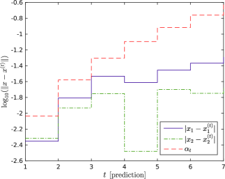
Figure 4: Mismatch between local and consolidated predictions.

Table I compares the proposed technique to [8]. The table reports the upper bound $\bar{k}$ on the number of iterations needed to achieve a suboptimal solution for Problem (2) and the level of suboptimality $\eta$. The table lists only the first four subproblems, which are the most significant due to the presence of active constraints in these subproblems. The method in [8] and our new proposed parallel algorithm produce a comparable behavior, thanks to an appropriate selection of the tightening parameters. The parallel algorithm, however, is able to achieve similar results to those in [8] using a smaller number of iterations. The larger values of $\bar{k}$ for [8] are probably caused by the value of the Lipschitz constant and by the problem conditioning, which affect the convergence requiring a higher accuracy for the solver. In particular, in our proposed framework, the DFG is applied to simpler problems characterized, in the worst case scenario, by a Lipschitz constant $\max_{t\!=\!0,\ldots,N}\{L_{\mu_{t}}\}=196$ and by a condition number $\max_{t\!=\!0,\ldots,N}\{\kappa_{t}\}=104$. In [8], the DFG solves a larger problem characterized by a Lipschitz constant $L_{s}=21994$ and by a condition number $\kappa_{s}=7020$. Hence, the modularity of our approach has positive implications on important properties for the convergence of the solver.

Table I lists the time required by the optimizer to return a suboptimal solution for Problem (2). To measure the performance, we implemented both algorithms in C on a Linux-based OS. We noticed that given the small size of the problem, running Algorithm 1 in parallel did not result in significant speedups compared to our algorithm running in serialized mode [9]. Nevertheless, in both cases, we registered a speedup (230x) compared to [8]. The modularity of the proposed algorithm is beneficial even for problems of small size, such as the one considered in this section for the comparison with [8]. We expect the benefits to be even more pronounced when considering problems of larger size.

TABLE I: PERFORMANCE ANALYSIS OF ALGORITHM 1 AND [8]. RESULTS SHOW THE MEDIAN OF 11 EXPERIMENTS.

Sample	Iterations (for subproblem)
time	$\bar{k}~{}{(\text{\cite[cite]{[\@@bibref{}{NecoaraOCAM}{}{}]}})}$	$\bar{k}_{0}$	$\bar{k}_{1}$	$\bar{k}_{2}$	$\bar{k}_{3}~{}~{}~{}\ldots$
0	$11\cdot 10^{4}$ (2.85 ms)	58931 (1.85 ms)	25	10	8
1	$12\cdot 10^{6}$ (302.84 ms)	18218 (0.57 ms)	3480	0	0
2	$11\cdot 10^{6}$ (267.56 ms)	2265 ( 0.07 ms)	0	0	0
	Suboptimality Level (for subproblem)
	$\eta~{}{(\text{\cite[cite]{[\@@bibref{}{NecoaraOCAM}{}{}]}})}$	$\eta_{0}$	$\eta_{1}$	$\eta_{2}$	$\eta_{3}~{}~{}~{}\ldots$
0	3.48	1.15	1.15	1.90	2.25
1	0.31	0.51	1.03	1.21	1.44
2	0.15	0.62	1.25	1.47	1.74

VII Conclusions

We proposed an algorithm tailored to MPC that guarantees recursive feasibility and closed-loop stability, when the solution of the MPC problem is computed using inexact solvers in a parallel framework. In particular, our algorithm combines ADMM and DFG methods and relies on an adaptive constraint-tightening strategy to certify the MPC law.

Our numerical analysis shows performance improvements compared to state-of-the-art nonparallel techniques [8]. Furthermore, our study shows that, for small-size problems, even if the solver is implemented in a serialized mode, there is substantial performance improvement with respect to the state of the art. We expect further benefits from the parallelization when the size of the problem increases. A scalability analysis of the proposed algorithm on many-core architectures is part of our ongoing work.

Appendix A Proof of Lemma 1

This section contains the proof of Lemma 1 presented in Section III-C.

Lemma 1.

Assume that there exists a Slater vector $\tilde{y}_{t}\in\mathbb{R}^{n+m}$ such that $G_{t}\tilde{y}_{t}+g_{t}<0$. Then, there exists $\epsilon_{t},\epsilon_{z_{t}},\epsilon_{z_{t+1}}\geq 0$, $\epsilon_{t}<{\min}_{j=1,\ldots,p_{t}}\{-(G_{t}\tilde{y}_{t}+g_{t})_{j}\}$, $\epsilon_{z_{t}},\epsilon_{z_{t+1}}>\epsilon_{t}$, such that the upper bound on $\mu^{*}_{t,\epsilon_{t}}$ is given by

$$\|\mu_{t,\epsilon_{t}}^{*}\|\leq 2{R_{d_{t}}}:=2{\frac{\mathbf{V}_{t}(\tilde{\xi}_{t})-d_{t}(\tilde{\mu}_{t})}{\min\limits_{j=1,\ldots,p_{t}+2n}\{[\Gamma_{t}]_{j}\}}},$$

where

$$\Gamma_{t}:=\begin{bmatrix}-(G_{t}\tilde{y}_{t}+g_{t})-\epsilon_{t}\operatorname{\mathbf{1}}_{p_{t}}\\ 2\rho(\epsilon_{z_{t}}-\epsilon_{t})\operatorname{\mathbf{1}}_{n}\\ 2\rho(\epsilon_{z_{t+1}}-\epsilon_{t})\operatorname{\mathbf{1}}_{n}\end{bmatrix}\in\mathbb{R}^{p_{t}+2n}$$

and $d_{t}(\tilde{\mu}_{t})$ is the dual function for the original subproblem (13) evaluated at $\tilde{\mu}_{t}\in\mathbb{R}^{p_{t}+4n}$.

The following inequality holds:

$$d(\tilde{\mu}_{t}) \leq\mathbf{V}_{t}(\tilde{\xi}_{t})+\mu_{t,\epsilon_{t}}^{*T}\nabla_{\mu_{t}}^{T}d_{t,\epsilon_{t}}(\mu_{t})$$

$$=\mathbf{V}_{t}(\tilde{\xi}_{t})+\lambda_{t,\epsilon_{t}}^{*T}(G_{t}\tilde{y}_{t}+g_{t}+\epsilon_{t}\mathbf{1}_{p_{t}})+$$

$$~{}~{}~{}+\rho w_{t,\epsilon_{t}}^{-*T}(-H_{1}\tilde{y}_{t}+z_{t}-\epsilon_{z_{t}}\mathbf{1}_{n}+\epsilon_{t}\mathbf{1}_{n})+$$

$$~{}~{}~{}+\rho w_{t,\epsilon_{t}}^{+*T}(H_{1}\tilde{y}_{t}-z_{t}-\epsilon_{z_{t}}\mathbf{1}_{n}+\epsilon_{t}\mathbf{1}_{n})+$$

$$~{}~{}~{}+\rho v_{t+1,\epsilon_{t}}^{-*T}(-H_{2}\tilde{y}_{t}+z_{t+1}-\epsilon_{z_{t+1}}\mathbf{1}_{n}+\epsilon_{t}\mathbf{1}_{n})+$$

$$~{}~{}~{}+\rho v_{t+1,\epsilon_{t}}^{+*T}(H_{2}\tilde{y}_{t}-z_{t+1}-\epsilon_{z_{t+1}}\mathbf{1}_{n}+\epsilon_{t}\mathbf{1}_{n})$$

$$\leq\mathbf{V}_{t}(\tilde{\xi}_{t})+\lambda_{t,\epsilon_{t}}^{*T}(G_{t}\tilde{y}_{t}+g_{t}+\epsilon_{t}\mathbf{1}_{p_{t}})+$$ (34)

$$~{}~{}~{}+2\rho~{}\text{max}\{w_{t,\epsilon_{t}}^{-*T},w_{t,\epsilon_{t}}^{+*T}\}(-\epsilon_{z_{t}}\mathbf{1}_{n}+\epsilon_{t}\mathbf{1}_{n})+$$

$$~{}~{}~{}+2\rho~{}\text{max}\{v_{t+1,\epsilon_{t}}^{-*T},v_{t+1,\epsilon_{t}}^{+*T}\}(-\epsilon_{z_{t+1}}\mathbf{1}_{n}+\epsilon_{t}\mathbf{1}_{n}),$$

where the last inequality takes into account that $w_{t,\epsilon_{t}}^{-*T},w_{t,\epsilon_{t}}^{+*T},v_{t+1,\epsilon_{t}}^{-*T},v_{t+1,\epsilon_{t}}^{+*T}\!\!\in\!\!\mathbb{R}^{n}_{+}$. Define $w_{t,\epsilon_{t}}^{*T}:=\max\{w_{t,\epsilon_{t}}^{-*T},w_{t,\epsilon_{t}}^{+*T}\}$ and $v_{t+1,\epsilon_{t}}^{*T}:=\max\{v_{t+1,\epsilon_{t}}^{-*T},v_{t+1,\epsilon_{t}}^{+*T}\}$. Consequently, using the definition of $w_{t}^{*T}$ and $v_{t+1}^{*T}$, the following holds:

$$\|\mu_{t,\epsilon_{t}}^{*}\|\leq\|[\lambda_{t,\epsilon_{t}}^{*T}~{}w_{t,\epsilon_{t}}^{*T}~{}v_{t+1,\epsilon_{t}}^{*T}]^{T}\|.$$ (35)

Furthermore, recalling that $\lambda_{t,\epsilon_{t}}^{*}\in\mathbb{R}^{p_{t}}_{+}$, $w_{t,\epsilon_{t}}^{*}\in\mathbb{R}^{n}_{+}$, and $v_{t+1,\epsilon_{t}}^{*}\in\mathbb{R}^{n}_{+}$, the following holds:

$$\|[\lambda_{t,\epsilon_{t}}^{*T}~{}w_{t,\epsilon_{t}}^{*T}~{}v_{t+1,\epsilon_{t}}^{*T}]^{T}\|\!\leq\![\lambda_{t,\epsilon_{t}}^{*T}~{}w_{t,\epsilon_{t}}^{*T}~{}v_{t+1,\epsilon_{t}}^{*T}]^{T}\!\!\operatorname{\mathbf{1}}_{p_{t}+2n}.$$ (36)

Hence, if we compute an upper bound for the vector $[\lambda_{t,\epsilon_{t}}^{*T}~{}w_{t,\epsilon_{t}}^{*T}~{}v_{t+1,\epsilon_{t}}^{*T}]^{T}$, we obtain an upper bound for $\|\mu_{t,\epsilon_{t}}^{*}\|$. Thus, from the inequality (34), it follows that:

$$\begin{bmatrix}\lambda_{t,\epsilon_{t}}^{*}\\ w_{t,\epsilon_{t}}^{*}\\ v_{t+1,\epsilon_{t}}^{*}\end{bmatrix}^{T}\underbrace{\begin{bmatrix}-(G_{t}\tilde{y}_{t}+g_{t})-\epsilon_{t}\mathbf{1}_{p_{t}}\\ 2\rho(\epsilon_{z_{t}}-\epsilon_{t})\mathbf{1}_{n}\\ 2\rho(\epsilon_{z_{t+1}}-\epsilon_{t})\mathbf{1}_{n}\end{bmatrix}}_{\Gamma_{t}}\leq\mathbf{V}_{t}(\tilde{\xi}_{t})-d(\tilde{\mu}_{t}).$$ (37)

Notice that choosing $\epsilon_{t}<\underset{j=1,\ldots,p_{t}}{\min}\{-(G_{t}\tilde{y}_{t}+g_{t})_{j}\}$, $\epsilon_{z_{t}},\epsilon_{z_{t+1}}>\epsilon_{t}$, i.e., according to the assumptions of the lemma, the elements of $\Gamma_{t}$ are all greater than zero.

Thus, using (35) and (36), it follows:

$$\frac{1}{2}\underset{j=1,\ldots,p_{t}+2n}{\min}\{[\Gamma_{t}]_{j}\}\|\mu_{t,\epsilon_{t}}^{*}\|\leq$$

$$\leq\begin{bmatrix}\lambda_{t,\epsilon_{t}}^{*}&w_{t,\epsilon_{t}}^{*}&v_{t+1,\epsilon_{t}}^{*}\end{bmatrix}\Gamma_{t}.$$ (38)

Consequently, the upper bound on the optimal Lagrange multiplier is given by:

$$\|\mu_{t,\epsilon_{t}}^{*}\|\leq 2\frac{\mathbf{V}_{t}(\tilde{\xi}_{t})-d(\tilde{\mu}_{t})}{\underset{j=1,\ldots,p_{t}+2n}{\min}\{[\Gamma_{t}]_{j}\}}.$$

Appendix B Proof of Lemma 2

This section contains the proof of Lemma 2 presented in Section IV-A.

Lemma 2.

Let the $t$-step-ahead consolidated prediction $\bar{x}_{t,\epsilon_{t}}$ be defined by (21) and assume that (22) holds. Then, there exists $\alpha_{t}\in\mathbb{R},\alpha_{t}\geq 0$, such that the mismatch between $\bar{x}_{t,\epsilon_{t}}$ and the state of $t$-th subproblem $\bar{x}_{t,\epsilon_{t}}^{(t)}$ is bounded, as follows:

$$|\bar{x}_{t,\epsilon_{t}}-\bar{x}_{t,\epsilon_{t}}^{(t)}|\leq\alpha_{t}.$$

In the following, we omit the dependence from $\epsilon_{t}$ to simplify the notation. The proof is constructive. For $t=0$, $x_{0}\equiv\bar{x}_{0}^{(0)}$. For $t=1$, $\bar{x}_{1}=Ax_{0}+B\bar{u}_{0}\equiv\bar{x}_{1}^{(0)}$, which is the 1-step-ahead state computed by the local subproblem 0, i.e., the subproblem associated to worker $\Pi_{0}$. Hence, the mismatch between $\bar{x}_{1}$ and $\bar{x}_{1}^{(1)}$ is simply given by

$$|\bar{x}_{1}-\bar{x}_{1}^{(1)}|\leq 2\epsilon_{z_{1}}=\alpha_{1}.$$

For $t\!=\!2,\ldots,N$, the following holds:

$$|\bar{x}_{2}-\bar{x}_{2}^{(2)}| =|\bar{x}_{2}-\bar{x}_{2}^{(1)}+\bar{x}_{2}^{(1)}-\bar{x}_{2}^{(2)}|$$

$$\leq|\bar{x}_{2}-\bar{x}_{2}^{(1)}|+|\bar{x}_{2}^{(1)}-\bar{x}_{2}^{(2)}|$$

$$\leq|A\bar{x}_{1}^{(0)}+B\bar{u}_{1}-A\bar{x}_{1}^{(1)}-B\bar{u}_{1}|+2\epsilon_{z_{2}}$$

$$\leq 2(\|A\|\epsilon_{z_{1}}+\epsilon_{z_{2}})=\alpha_{2},$$

$$~{}\vdots$$

$$|\bar{x}_{N}-\bar{x}_{N}^{(N)}|\leq 2(\|A^{N-1}\|\epsilon_{z_{1}}+\|A^{N-2}\|\epsilon_{z_{2}}$$

$$\quad\quad\quad\quad\quad\quad+\ldots+\epsilon_{z_{N}})=\alpha_{N},$$

which proves the lemma.

Appendix C Proof of Lemma 3

This section contains the proof of Lemma 3 presented in Section IV.

Lemma 3.

Consider the following IT subproblems:

$$\mathbf{V}^{*}_{\gamma_{t}}\!=\!\min_{\xi_{t}}~{}\mathbf{V}_{t}(\xi_{t})~{}\text{s.t.:}~{}G_{\xi_{t}}\xi_{t}+g_{\xi_{t}}+\mathbf{\gamma}_{t}\leq 0,$$ (39)

for $t\!=\!0,\ldots,N$, where $\gamma_{t}$$:=[$$(|C_{t}|\alpha_{t}\operatorname{\mathbf{1}}_{n}+\epsilon_{t}\operatorname{\mathbf{1}}_{p_{t}})^{T}$ $\epsilon_{t}\operatorname{\mathbf{1}}^{T}_{4n}]^{T}$. Given the assumptions of Lemma 1 and the existence of $\alpha_{t}$ for all $t\!=\!1,\ldots,N$ according to Lemma 2. Then, for each subproblem, there exist $\epsilon_{t}\geq 0$, $\epsilon_{z_{t}},\epsilon_{z_{t+1}}>\epsilon_{t}$ such that the upper bound on the optimal Lagrange multiplier associated with the IT subproblems (39) is described by

$$\|\mu_{t,\gamma_{t}}^{*}\|\leq 2\mathcal{R}_{t}:=2{\frac{\mathbf{V}_{t}(\tilde{\xi}_{t})-d_{t}(\tilde{\mu}_{t})}{\min_{j=1,\ldots,p_{t}+2n}\{[\Gamma_{\alpha_{t}}]_{j}\}}},~{}t\!=\!0,\ldots,N,$$

$$\Gamma_{\alpha_{t}}:=\begin{bmatrix}-(G_{t}\tilde{y}_{t}+g_{t})-|C_{t}|\alpha_{t}\operatorname{\mathbf{1}}_{n}-\epsilon_{t}\mathbf{1}_{p_{t}}\\ 2\rho(\epsilon_{z_{t}}-\epsilon_{t})\mathbf{1}_{n}\\ 2\rho(\epsilon_{z_{t+1}}-\epsilon_{t})\mathbf{1}_{n}\end{bmatrix}.$$

This lemma follows from Lemma 1 applied to the subproblems (25). From inequality (37) formulated for subproblem (25), the following must hold

$$\begin{bmatrix}\lambda_{t,\epsilon_{t}}^{*}\\ w_{t,\epsilon_{t}}^{*}\\ v_{t+1,\epsilon_{t}}^{*}\end{bmatrix}^{T}\underbrace{\begin{bmatrix}-(G_{t}\tilde{y}_{t}+g_{t})-|C_{t}|\alpha_{t}\operatorname{\mathbf{1}}_{n}-\epsilon_{t}\mathbf{1}_{p_{t}}\\ 2\rho(\epsilon_{z_{t}}-\epsilon_{t})\mathbf{1}_{n}\\ 2\rho(\epsilon_{z_{t+1}}-\epsilon_{t})\mathbf{1}_{n}\end{bmatrix}}_{\Gamma_{\alpha_{t}}}\leq$$

$$\leq\mathbf{V}_{t}(\tilde{\xi}_{t})-d(\tilde{\mu}_{t}).$$

Hence, in order to satisfy the inequality above, we can select the relaxation parameters $\epsilon_{z_{t}}$ and the tightening parameters $\epsilon_{t}$ according to the assumption of the lemma for $t\!=\!0,\ldots,N$, i.e., the following must hold:

(i) $$\frac{1}{2}\!\!\min\limits_{j=1,\ldots,p_{t}}\!\!\{-(G_{t}\tilde{y}_{t}+g_{t})_{j}\}\!\!\geq\!\!\!\max\limits_{j=1,\ldots,p_{t}}\!\!\!\big{\{}\sum_{i=1}^{n}|[C_{t}]_{j,i}|\big{\}}\alpha_{t}+\epsilon_{t}$$

(ii) $$\max\limits_{j=1,\ldots,p_{t}}\!\!\!\big{\{}\sum_{i=1}^{n}|[C_{t}]_{j,i}|\big{\}}\alpha_{t}+\epsilon_{t}>0$$

(iii) $$\epsilon_{z_{t}},\epsilon_{z_{t+1}}\geq\epsilon_{t}\geq 0,$$

where $\tilde{y}_{t}$ is a strictly feasible solution for the original $t$-th subproblem. Hence, there exists $\mathcal{R}_{t}$ such that the upper bound on the optimal Lagrange multiplier $\mu_{t,\gamma_{t}}^{*}$ is defined as follows:

$$\|\mu_{t,\gamma_{t}}^{*}\|\leq\frac{\mathbf{V}_{t}(\tilde{\xi}_{t})-d(\tilde{\mu}_{t})}{{\underset{j=1,\ldots,p_{t}+2n}{\min}\{[\Gamma_{t}{\alpha_{t}}]\}}}.$$

Appendix D Proof of Theorem 2

This section contains the proof of Theorem 2 presented in Section V.

Theorem 2.

Assuming that there exist $\epsilon_{t}$ ($t\!=\!0,\ldots,N$) and $\epsilon_{z_{t}}$ ($t\!=\!1,\ldots,N$) selected according to Lemma 3, then the following holds:

$$\mathcal{V}^{*}\leq\mathbf{V}_{\gamma}\leq\mathcal{V}^{*}+2\sum_{t=0}^{N}\mathcal{R}_{t}\sqrt{p_{t}}\bar{\gamma}_{t},$$

where $\bar{\gamma}_{t}:=\epsilon_{t}+\max\limits_{j=1,\ldots,p_{t}}\!\!\!\big{\{}\sum_{i=1}^{n}|[C_{t}]_{j,i}|\big{\}}\alpha_{t}$.

Due to the tightening of the original inequality constraints, $\mathbf{V}_{\gamma}\geq\mathcal{V}^{*}$, given that, as proved in Section IV-B, the feasible region of the tightened subproblems is inside the one of the original subproblems.

Recall that the consolidated prediction satisfies the equality constraints (2b) by construction. Hence, the following holds:

$$\mathbf{V}_{\gamma}\!\!\leq\!\! \sum\limits_{t=0}^{N}\big{[}\max\limits_{\lambda\geq 0}(\min\limits_{x_{t},u_{t}}\mathcal{V}_{t}(x_{t},u_{t})+\left\langle\lambda,C_{t}x_{t}+D_{t}u_{t}+g_{t}\right\rangle)$$

$$\quad\quad+\left\langle\lambda_{\gamma_{t}}^{*},[I_{{p_{t}}}~{}0]\gamma_{t}\right\rangle\big{]}$$

$$\leq \mathcal{V}^{*}+2\sum\limits_{t=0}^{N}\mathcal{R}_{t}\sqrt{p_{t}}(\epsilon_{t}+\!\!\!\max\limits_{j=1,\ldots,p_{t}}\!\!\!\big{\{}\sum_{i=1}^{n}|[C_{t}]_{j,i}|\big{\}}\alpha_{t}).$$

where $[I_{{p_{t}}}~{}0]\gamma_{t}$ selects the first $p_{t}$ components of the vector $\gamma_{t}$.

Appendix E Proof of Lemma 4

This section contains the proof of Lemma 4 presented in Section V.

Lemma 4.

Let $\bar{y}_{\gamma}$ be defined as $\bar{y}_{\gamma}:=[\bar{y}_{0,\gamma_{0}}^{T}\ldots\bar{y}_{N,\gamma_{N}}^{T}]=[(x_{0}^{T}~{}\bar{u}_{0,\gamma_{0}}^{T})\ldots(\bar{x}_{N-1,\gamma_{N-1}}^{T}~{}\bar{u}_{N-1,\gamma_{N-1}}^{T})~{}(\bar{x}_{N,\gamma_{N}}^{T}))]^{T}$. Then, $\tilde{y}^{+}$ at the next problem instance, is given by:

$$\tilde{y}^{+} =[\bar{y}_{{\gamma}_{[2:N+1]}}((A+BK_{f})\bar{x}_{N,\gamma_{N}})^{T}]^{T}$$

We can use a similar argument as the one of Lemma 4.2 in [8], recalling that $C_{t}=C$ for $t\!=\!0,\ldots,N-1$, $C_{t}=F_{N}$ for $t=N$, $D_{t}=D$ for $t\!=\!0,\ldots,N-1$, $D_{t}=0$ for $t=N$, and $\mathcal{X}_{N}\subseteq\mathcal{X}$ according to Assumption 2.

References

• [1] S. D. Cairano, M. Brand, and S. A.  Bortoff, “Projection-free parallel quadratic programming for linear model predictive control”. International Journal of Control, vol. 86, no. 8, pp. 1367–1385, 2013.
• [2] M. Kögel and R. Findeisen, “Parallel solution of model predictive control using the alternating direction multiplier method”, Proc. of the IFAC Conference on NMPC, vol. 4, no. 1, pp. 369–374, 2012.
• [3] G. Stathopoulos, T. Keviczky, and Y. Wang, “A hierarchical time-splitting approach for solving finite-time optimal control problems”, Proc. of the ECC, pp. 3089–3094, 2013.
• [4] S. Boyd et al. “Distributed optimization and statistical learning via the alternating direction method of multipliers”. In Foundations and Trends® in Machine Learning, vol. 3, no. 1, pp. 1–122, 2011.
• [5] D. P. Bertsekas, “Constrained optimization and Lagrange multiplier methods”. Athena Scientific, 1996.
• [6] M. Kögel and R. Findeisen, “Fast predictive control of linear, time-invariant systems using an algorithm based on the fast gradient method and augmented Lagrange multipliers”, Proc. of the IEEE CCA, pp. 780–785, 2011.
• [7] M. Rubagotti, P. Patrinos and A. Bemporad, “Stabilizing Linear Model Predictive Control Under Inexact Numerical Optimization”, In IEEE Trans. on Automatic Control, vol. 59, no. 6, pp. 1660–1666, 2014.
• [8] I. Necoara, L. Ferranti, and T. Keviczky, “An adaptive tightening approach to linear model predictive control based on approximation algorithms for optimization”, Optimal Control Applications and Methods, DOI: 10.1002/oca.2121, http://dx.doi.org/10.1002/oca.2121, to appear in 2015.
• [9] M. Voss and R. Eigenmann. “Reducing parallel overheads through dynamic serialization”, Proc. of the 13th IPDPS, pp. 88–92, 1999.
• [10] Y. Nesterov, “Smooth minimization of non-smooth functions”, Mathematical Programming, vol. 103, pp. 127–152, 2004.
• [11] M. Herceg, M. Kvasnica, C.N. Jones, and M. Morari. “Multi-Parametric Toolbox 3.0”, Proc. of the ECC, pp. 502–510, 2013.
• [12] A. Nedić and A. Ozdaglar. “Approximate primal solutions and rate analysis for dual subgradient methods”, SIAM Journal on Optimization, vol. 19, no. 4, pp. 1757–1780, 2009.
• [13] J.B. Rawlings and D.Q. Mayne. “Model Predictive Control: Theory and Design”, Nob Hill Publishing, 2009.
• [14] M. Rubagotti, P. Patrinos, and A. Bemporad. “Stabilizing Embedded MPC with Computational Complexity Guarantees”, Proc. of the ECC, pp. 3065–3070, 2013.