Griffiths phases and localization in hierarchical modular networks

Abstract

We study variants of hierarchical modular network models suggested by Kaiser and Hilgetag [Front. in Neuroinform., 4 (2010) 8] to model functional brain connectivity, using extensive simulations and quenched mean-field theory (QMF), focusing on structures with a connection probability that decays exponentially with the level index. Such networks can be embedded in two-dimensional Euclidean space. We explore the dynamic behavior of the contact process (CP) and threshold models on networks of this kind, including hierarchical trees. While in the small-world networks originally proposed to model brain connectivity, the topological heterogeneities are not strong enough to induce deviations from mean-field behavior, we show that a Griffiths phase can emerge under reduced connection probabilities, approaching the percolation threshold. In this case the topological dimension of the networks is finite, and extended regions of bursty, power-law dynamics are observed. Localization in the steady state is also shown via QMF. We investigate the effects of link asymmetry and coupling disorder, and show that localization can occur even in small-world networks with high connectivity in case of link disorder.

Introduction

In neuroscience, the criticality hypothesis asserts that the brain is in a critical state, at the boundary between sustained activity and an inactive regime. Theoretical and experimental studies show that critical systems exhibit optimal computational properties, suggesting why criticality may have been selected in the evolution of the nervous system [1]. Although criticality has been observed in cell cultures [2, 3], brain slices and anesthetized animals [4, 5], the debate regarding criticality in alert animals and humans continues [6, 7, 8]. Thus the criticality hypothesis remains controversial in brain science; for a review see [9].

Normally, for a system to be at criticality, certain control parameters need to be tuned precisely, raising the perennial question of how such tuning is achieved in the absence of outside intervention. The possibility of self-tuning is well known in statistical physics; the paradigm of self-organized criticality (SOC) has been studied since the pioneering work of [10]. Simple homogeneous models such as the stochastic sandpile exhibit criticality with power laws both in statics and dynamics. This has been understood as the result of a control mechanism that forces the system to an absorbing-state phase transition [11]

Real nervous systems, however, are highly inhomogeneous, so that one must take into account the effects of heterogeneities. It is well known in statistical physics that disorder can cause rare-region (RR) effects [12] that smear the phase transitions. These effects can make a discontinuous transition continuous, or generate so-called Griffiths phases (GP) [13], in which critical-like power-law dynamics appears over an extended region around the critical point. In these regions, moreover, non-Markovian, bursty behavior can emerge as a consequence of a diverging correlation time. The inter-communication times of the nodes (which possess no internal memory) follow a fat-tailed distribution [14]. Thus, heterogeneities widen the critical region and can contribute to the occurrence of power laws. This provides an alternative mechanism for critical-like behavior without fine tuning, although attaining the GP does require some rough tuning, of the sort that is not difficult to find in biological systems.

It was shown recently that the topological heterogeneity of the underlying networks can result in GPs in finite-dimensional systems [15] and can be a reason for the working memory in the brain [16]. Although many networks exhibit the small-world property and so have an infinite topological dimension, naturally occurring networks are always finite, exhibit cutoffs, and therefore GPs can be expected as a consequence of inhomogeneous topology [17].

Many real networks can be partitioned seamlessly into a collection of modules. Each module is expected to perform an identifiable task, separate from the function of others [18]. It is believed that the brain is organized hierarchically into modular networks across many scales, starting from cellular circuits and cortical columns via nuclei or cortical areas to large-scale units such as visual or sensory-motor cortex. At each level, connections within modules are denser than between different modules [19, 20, 21, 22]. Although empirical data confirm this modular organization on some scales [23], the detailed organization of brain networks is not yet experimentally accessible.

Two particular kinds of hierarchical modular networks (HMN-1,HMN-2) model were proposed and investigated numerically and analytically in [24]. On large-world HMNs, which imply a finite topological dimension $D$, models of the spread of activity exhibit power-law dynamics and rare region effects. However, these power laws are system-size dependent, so that true GP behavior has not yet been proven. These authors also simulated spreading on empirical brain networks, such as the human connectome and the nervous system of C. elegans. Available empirical networks are much smaller than the synthetic ones and deviations from power laws are clearly visible. Both anatomical connections [19] and the synchronization networks of cortical neurons [27] suggest small-world topology [26]. The brain network modules of [24] are weakly coupled in such a way that these HMNs are near the percolation threshold, as in the case of the models introduced in [15]. Note, however that requiring the network to be near percolation again raises tuning and robustness issues. Having weaker ties would lead to fragmented networks, while stronger ties result in infinite $D$ and the absence of a GP. In the present work we do not assume such fine tuning: we maintain a high density of short edges, rendering the networks well connected. Another way of preserving the integrity of HMN networks with finite dimension involves the random tree-like structures studied here.

To study synchronization [28], commonly expected in brain dynamics, the Kuramoto model [29] has been implemented [30] on the same networks as studied in [24]. In this case even weaker rare-region effects were found, resulting in stretched exponential dynamics. One of the main purposes of our study is to delineate conditions a GP. While the networks studied are of finite size, repeating the process on many network realizations and averaging over them, we clearly see convergence towards GP dynamics. We assume that multiple random network realizations may occur in the brain over time, due to reconfigurations of the synapses or as a consequence of weakly coupled sub-modules and changes in overall intensity of connections between different brain regions due to neuromodulation.

In addition to the dimension, other topological features, which have yet to be studied systematically, may also influence RR effects. The clustering coefficient, defined as

$$C(N)=1/N\sum_{i}\frac{2n_{i}}{k_{i}(k_{i}-1)}\ ,$$ (1)

where $n_{i}$ denotes the number of direct links interconnecting the $k_{i}$ nearest neighbors of node $i$, exhibits different scaling behavior in modular networks than in unstructured networks. While in SF networks it decays as $C(N)\sim N^{-3/4}$ and in random networks as $C(N)\sim N^{-1}$, in HMNs it is constant. Furthermore, while in SF networks the clustering is degree-number independent, in HMNs it decays as $C(k)\sim k^{-\beta}$, with $\beta$ in the range 0.75 - 1 [31]. This means that the higher the node degree, the smaller is its clustering coefficient, possibly reducing its infectiousness in an epidemic process. This suggests an enhancement of localization as in SF models with disassortative weighting schemes [32].

In this work we study spreading models defined on HMNs embedded in 2D space, and investigate how various inhomogeneities (topological or intrinsic) contribute to the occurrence of localization and GPs. We begin by considering purely topological heterogeneity; later we study cases with disorder in the connections as well. It is well known that intrinsic link disorder can appear as the consequence of asymmetry, connecting nodes in the cortex (see [33]). It has also been demonstrated that weights can vary over 4-6 orders of magnitude; most (including the majority of long-range connections) are actually quite weak [34].

The relation of RR effects to localization in the steady state has been studied recently [17]. Here we discuss localization results obtained via a quenched mean-field (QMF) approximation.

In addition to serving as models of brain connectivity, hierarchical modular networks are abundant in nature. They occur in social relations [35], in the WWW [36], metabolic [37] and information systems [38] for example. Thus the results reported here should find application in these and related areas.

Hierarchical modular networks

Recent studies indicate that activity in brain networks persists between the extremes of rapid extinction and global excitation. This so-called limited sustained activity (LSA) does not occur in spreading models defined on structureless, small-world networks. On the other hand, brain networks are known to exhibit hierarchical modular structure. This motivated Kaiser and Hilgetag (KH) to perform numerical studies on such networks, to investigate topological effects on LSA [39]. Their hierarchical model reflects general features of brain connectivity on large and mesoscopic scales. Nodes in the model were intended to represent cortical columns rather than individual neurons. The connections between them were taken as excitatory, since there appear to be no long-distance inhibitory connections within the cerebral cortex [40].

Kaiser and Hilgetag generated networks beginning at the highest level, and adding modules to the next lower level, with random connectivity within modules. They explored hierarchical networks with different numbers of levels, and numbers of sub-modules at each level. The average degree (over all nodes in the network) was set to $\langle k\rangle=50$, motivated by experimental studies. They investigated different topologies by varying the edge density across the levels. All the networks studied by KH are of small-world type, i.e., they have an infinite topological dimension.

The spreading model investigated by KH is a two-state threshold model, in which, at each time step, inactive nodes are activated with probability $\lambda$ if at least $m$ of their neighbors are currently active, and active nodes deactivate spontaneously with probability $\nu$. This model is very similar to reaction-diffusion models known in statistical physics [41, 42, 43], with a synchronous cellular automaton (SCA) updates. Starting from an initial state in which a localized set of nodes is active, these authors followed the density of active sites and their localization up to $t\simeq 200$ time steps on networks of sizes $N\leq 512$.

Kaiser and Hilgetag found that LSA can be found in a larger parameter range in HMNs, as compared with random and non-hierarchical small-world networks. The optimal range of LSA was found in networks in which the edge density increased from the top level ($l=l_{max}$) to the bottom ($l=l_{1}$). Such topologies foster activity localization and rare-region effects.

In this paper we investigate HMNs which possess increasing edge density from top to bottom levels, as did KH, but with finite topological dimension. We will show that although localization is seen in small world networks, to observe GPs, with power-law dynamics, we need networks of finite topological dimension.

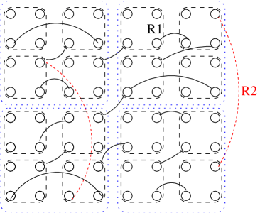
Figure 1: Two lowest levels of the HMN2d hierarchical network construction. Dashed lines frame bottom level nodes, which are fully connected there, dotted lines frame the nodes of the next level. The solid lines denoted R1 are randomly chosen connections among the bottom level modules, ensuring single connectedness of the network, while those denoted R2 provide random connections on the next level. Links can be directed.

To generate a hierarchical modular network, we define $l_{max}$ levels on the same set of $N=4^{l_{max}}$ nodes; on the $l^{th}$ level we define $4^{l}$ modules. We achieve this by splitting each module into four equal sized modules on the next level, as if they were embedded in a regular, two-dimensional (2d) lattice (see Figure 1). The probability $p_{l}$ that two nodes are connected by an edge follows $p_{l}\simeq b2^{-sl}$ as in [39], where $l$ is the greatest integer such that the two nodes are in the same module on level $l$. After selecting the number of levels and nodes we fix the average node degree, $b=\langle k\rangle/2$, and generate the adjacency matrix $A$ by proceeding from the highest to the lowest level. We fill the submatrices with zeros and ones and copy them to appropriate diagonal locations of $A$. We allow unidirectional connections, which is more realistic. In fact, disorder associated with the link orientations turns out to be necessary to observe GPs. Finally, we connect the lowest-level modules with an edge, chosen randomly from nodes of $l_{1}$. This provides a short-linked base lattice that guarantees connectivity.

In a preliminary study, the extra edges, corresponding to the base lattice, were not added. The resulting networks typically consist of a large number of isolated connected components; the GP effects observed in these structures are a consequence of fragmented domains of limited size. Measurements of axon-length distributions in several real neural networks show a large peak at short distances followed by a long flat tail. Thus there is a dense set of local edges in addition to a sparse network of long-range connections, best fit by an exponential function [44]. Typical estimates indicate that $\simeq 90\%$ of all cortical connections are formed at the local level (i.e., within a radius of $0.5$mm); only the remainder leave the local gray matter and project to remote targets. Therefore, we also investigate a variant of HMN2d networks in which the lowest-level modules are fully connected, and there is a single link among the nodes of modules on level $l_{2}$. To broaden further the range of structures, we study hierarchical modular trees (HMTs), which possess the minimum number of edges required for connectivity, and so have no loops. Construction of HMTs is described in the Supplementary material.

Relation to Benjamini-Berger networks

Due to the embedding, there is a correspondence with Benjamini-Berger (BB) networks [45]. BB networks are generated on Euclidean lattices, with short links connecting nearest neighbors. In addition, the network contains long links, whose probability decays algebraically with Euclidean distance $R$:

$$p(R)\sim R^{-s}\ .$$ (2)

Here we consider modified BB networks, in which the long links are added level by level, from top to bottom, as in [39]. The levels : $l=1,...,l_{max}$ are numbered from the bottom to top. The size of domains, i.e., the number of nodes in a level, grows as $N_{l}=4^{l}$ in the 4-module construction, related to a tiling of the two dimensional base lattice. Due to the approximate distance-level relation, $R\simeq 2^{l}$, the long-link connection probability on level $l$ is:

$$p_{l}=b\left(\frac{1}{2^{s}}\right)^{l}\ .$$ (3)

Here $b$ is related to the average degree of a node $\langle k\rangle$.

It is known that in a one-dimensional base lattice the BB construction results in a marginal case, $s=2$, in which the topological dimension is finite and changes continuously with $b$. For $s<2$ we have small world networks, while for $s>2$ the the topological dimension is the same as the base lattice ($d=1$) in BB networks. The HMN-1 networks studied by Moretti and Muñoz [24] are similar to the BB model, without the 1d base lattice, but with the inclusion of a HMN topology. These authors simulated spreading models on HMN-1 with finite topological dimension at $p_{l}\sim(\frac{1}{4})^{l}$ and found GPs. Given the above mapping, this result is not very surprising, because this HMN corresponds to the $s=2$ case, staying close to the percolation threshold of the network. To ensure connectivity, Moretti and Muñoz added extra links to the large connected components [24]; they assert that the topological dimension remains finite, despite the additional links. In networks with finite sizes this is certainly true, however in the infinite size limit such a system is also infinite dimensional, so that we don’t expect true GPs. For the HMN-2, the number of connections between blocks at every level is a priori set to a constant value. In this case numerics of [24, 25] suggest GP effects.

Here we embed the HMNs in 2d base lattices, which is closer to the real topology of cortical networks. In this case the threshold for marginality (i.e., continuously changing dimension and exponents) is expected to be at $s=4$. We confirm this by explicit measurements of the topological dimension. Furthermore, we study two-dimensional HMNs with different $s$ values and find GP effects for finite topological dimensions, both at the percolation threshold (for $s=3$), and for $s=6$, where the tail distribution of the link lengths decays very rapidly, in agreement with empirical results for axon lengths.

In addition to the CP ($m=1$), we also consider threshold models ($m\geq 2$), which are expected to be more realistic for neuronal systems.

Dimension measurements

To measure the dimension of the network we first compute the level structure by running a breadth-first search from several, randomly selected seeds. We count the number of nodes $N(r)$ with chemical distance $r$ or less from the seeds and calculate averages over the trials. We determined the dimension of the network from the scaling relation $N\sim r^{d}$, by fitting a power-law to the data for $N(r)$.

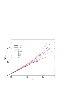
Figure 2: Number of nodes within the chemical distance $r$ in the $s=3$ HMN2d models with $l_{max}=9$. Different curves correspond to different parameters: $b=\langle k\rangle/2$ as indicated. The dashed line shows a power-law fit for $b=2$, with $N(r)\sim r^{1.4}$, suggesting a topological dimension of $d=1.4$ at the percolation threshold.

At $s=3$ we observe a percolation threshold near $\langle k\rangle=4$, for which the topological dimension is finite: $d\simeq 1.4$ (see Figure 2). Note that the curves with large $\langle k\rangle$ exhibit saturation, corresponding to a finite-size effect. The case $s=4$ appears to correspond to a marginal dimension, for which, above the percolation threshold $\langle k\rangle>6$, one observes a continuously varying topological dimension (see Figure 3). A more detailed, local slopes analysis via the effective topological dimension

$$d_{\rm eff}=\frac{\ln[N(r))/N(r^{\prime})]}{\ln(r/r^{\prime})}\ ,$$ (4)

is shown in the inset of Figure 3, where $r$ and $r^{\prime}$ are neighboring measurement points. Saturation to $s$-dependent dimensions can be read off the plot for $r>100$.

Figure 3: Number of nodes within chemical distance $r$ in HMN2d networks with $s=4$ and $l=9$ levels. Different curves correspond to different $b=\langle k\rangle/2$ values as indicated. Inset: local slopes $d_{eff}$ of the $N(r)$ curves, defined in equation. 4.

Random hierarchical trees also exhibit a finite topological dimension. Figurere 4 shows $N(r)$ for a set of ten independent random trees. The average of $N(r)$ over the set of ten trees follows a power law to good approximation, with $d\simeq 0.72$. (Note that in this case $N(r)$ is an average over all nodes.) For regular trees, by contrast, $N(r)$ grows exponentially with $r$, as shown in Figure 5. Thus the regular tree construction results in a structure with infinite topological dimension.

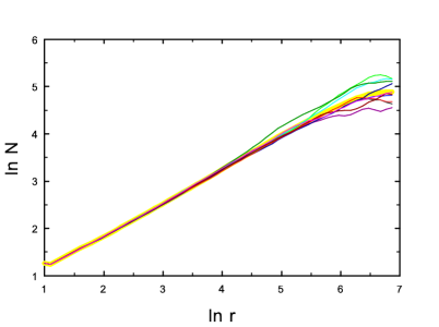
Figure 4: Number of nodes within chemical distance $r$ in a set of ten random hierarchical trees with 262144 nodes (thin curves). The broad yellow curve is an average over the set of ten structures.

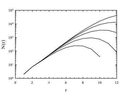
Figure 5: Number of nodes within chemical distance $r$ in regular hierarchical trees with 1024, 4096, …, 262144 nodes (lower to upper curves).

Dynamic simulations

Contact process

The contact process (CP) [46, 47], a Markov process defined on a network, can be interpreted as a simple model of information spreading in social [48], epidemic spreading [49, 50, 51], or in brain networks [24]. In the CP sites can be active or inactive. Active sites propagate the activity to their neighbors at rate $\lambda/k$, or spontaneously deactivate with rate $\nu=1$ (for simplicity).

We perform extensive activity-decay simulations for HMN2d models with $2b=\langle k\rangle=4$ and maximum levels: $l_{max}=8,9,10$. In these networks we use directed links between nodes, similar to real nervous systems. We follow $\rho(t)$ in $10-100$ runs for each independent random network sample, starting from fully active initial states, and averaging $\rho(t)$ over thousands of independent random network samples for each $\lambda$. In the marginal long-link decay case at $s=4$, a clear GP behavior is found (see Figure 6).

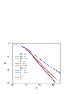
Figure 6: CP on asymmetric HMN2d networks with $s=4$: decay of activity for $\lambda$ values as indicated. System sizes $l_{max}=8,9,10$ (thin, medium, and thick lines, respectively). Size-independent power laws are evidence of a Griffiths phase.

We show that a GP can occur for more general parameters than those studied in [24], by following the density decay in networks with $s=3$ and $\langle k\rangle=4$ (i.e., at the percolation threshold). Size-independent, nonuniversal power laws can be seen in Figure 7.

When we increase the average degree $\langle k\rangle$, the GP shrinks to a smaller range of $\lambda$ values, as in [15], tending toward a simple critical phase transition. However, it is hard to determine at precisely which value of $\langle k\rangle$ this happens. We note that the connectivity of the network is not assured, without the addition of extra links. Strictly speaking, however, with this extension $s\leq 4$ networks become infinite-dimensional in the $N\to\infty$ limit.

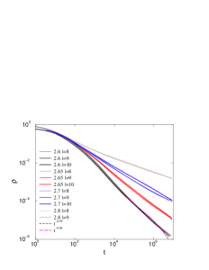
Figure 7: CP on asymmetric HMN2d networks as in Figure 6, but for $s=3$.

More importantly, GPs are also found in networks connected on the base level via short edges. We study the activity decay for $s=6$, which corresponds to fast decaying tail distribution for the long links, preserving finite topological dimension $d$. In this construction the average degree at the bottom level is $\langle k\rangle\simeq 6$, decreasing systematically with $l$, so that $\langle k\rangle\simeq 1$ for $l_{max}$. Note that that the ratio of short to long links is $\sim 0.11$, in agreement with results for real neural networks [44]. Simulations again yield size-independent power-law decay curves, confirming GP behavior, as shown in Figure 8.

We also determined the effective decay exponent in the usual manner (see [43]), via

$$\alpha_{\rm eff}(t)=-\frac{\ln[\rho(t)/\rho(t^{\prime})]}{\ln(t/t^{\prime})}\ ,$$ (5)

where $\rho(t)$ and $\rho(t^{\prime})$ are neighboring data points. The critical point can be located at $\lambda_{c}=2.53(1)$, showing mean-field scaling: $\rho(t)\sim t^{-1}$. Above this threshold power-laws can still be seen for smaller sizes ($l_{max}=8,9$), up to $\lambda\simeq 2.55$, but corrections to scaling become stronger; the curves for $l_{max}=10$ exhibit saturation. This is surprising, because in a disordered system with short ranged interactions one would expect a critical phase transition with an ultra-slow, logarithmic scaling. However, recent studies of the CP in higher dimensions find mean-field criticality and GP [52]. Our result suggests that the topological heterogeneity generated by the long edges is not strong enough to induce an infinite-randomness fixed point. Otherwise we must assume very strong corrections to scaling in this case.

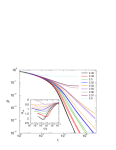
Figure 8: CP on asymmetric HMN2d networks with $s=6$ and $\langle k\rangle\simeq 4$: decay of activity for $\lambda$ values as indicated. System sizes as in Figure 6. Size-independent power laws are observed for $2.45<\lambda<2.53$. Inset: local slopes of the curves in the main plot. In the GP $\alpha_{eff}$ tends to nonuniversal values with logarithmic corrections. At $\lambda_{c}=2.53(1)$ we observe convergence to $\alpha_{eff}=1$; above this threshold the effective exponents of larger systems veer upwards toward zero as $t$ tends to infinity.

Disorder due to the randomly chosen orientations of the links turns out to be relevant. For symmetric links our simulations yield nonuniversal power laws, which appear to be sensitive to the system size, suggesting the lack of a true GP in the infinite-size limit.

Burstyness in the CP

We study the distribution of inter-event times in the CP on asymmetric, HMN2d networks with $s=6$, in a manner similar to that described in [14]. Starting from fully active states, on networks of size $l_{max}=10$, we measured $\langle\Delta t\rangle$ between successive activation attempts. We followed the evolution up to $t_{max}=2^{18}$ Monte Carlo steps (MCs), averaging over $1000-2000$ independent random networks with $10-100$ runs for each. Througout this paper time is measured by MCs. As Figure 9 shows, fat-tailed distributions, $P(\Delta t)\sim(\Delta t)^{-x}$, emerge in the GP for $2.46<\lambda<2.6$, while $P(\Delta t)$ decays exponentially outside this region. The slopes of the decay curves are determined via least-squares fits in the window $20<\Delta t<7000$. For $\lambda=2.5$ we find $x=1.753(4)$, while for $\lambda=2.52$ the exponent is slightly larger: $x=1.81(1)$. These values are close to the auto-correlation exponent of the critical $1+1$ dimensional CP as in [14], but exhibit deviations due to the heterogeneities. This is understandable, since the effective dimension of this HMN2d is close to one. The scaling variable $P^{*}(\Delta t)\equiv(\Delta t)^{1.79}P(\Delta t)$ exhibits log-periodic oscillations. This is the consequence of the modular structure of the network. Furthermore, as in other GP models, logarithmic corrections to scaling are expected.

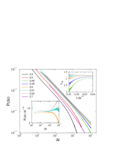
Figure 9: CP on asymmetric HMN2d networks with $s=6$. Main plot : probability distribution, $P(\Delta t)$, of inter-event times for $\lambda$ values as indicated; system size $l_{max}=10$. Power-law tails are evident for $2.46<\lambda<2.6$, with continuously changing exponents. Right inset: local slopes of the same curves, defined similarly as in equation (5) for: $\lambda=2.46,2.48,2.5,2.52,2.7$. Left inset: $P^{*}(\Delta t)\equiv(\Delta t)^{1.79}P(\Delta t)$ for $\lambda=2.5,2.51,2.52$.

We expect similar nonuniversal, control parameter dependent tails in $P(\Delta t)$ in the GPs exhibited by the other HMN2d networks. Furthermore, as shown in [14], power-law distributions should arise for other initial conditions, such as localized activity. This suggests that bursty inter-communication events in brain dynamics arise spontaneously near the critical point, in the GP.

CP on random hierarchical trees

We simulate the CP with symmetric links on random hierarchical trees (RHTs) of 262 144 nodes. We first perform quasistationary (QS) simulations [53], of the CP on a single RHT. For one structure this yields $\lambda_{c}\simeq 2.72$; for another, independently generated structure of the same kind, we find $\lambda_{c}\simeq 2.76$.

Our principal interest is in the decay of activity starting from all nodes active. The decay of activity on a single RHT appears to follow the scenario familiar from the CP on regular lattices: power-law decay is observed at $\lambda_{c}$ but not at nearby values, as illustrated in Figure 10. The randomness associated with a single RHT appears to be insufficient to generate a Griffiths phase.

By contrast, evidence of a GP is found if we average over many RHTs. The activity averaged over a large set ($10^{3}$ - $10^{4}$) of independent realizations, each on a different RHT, shown in Figure 11, decays asymptotically as a power-law over a fairly broad range of subcritical $\lambda$ values. The decay exponent $\alpha$ extrapolates to zero at $\lambda=2.760(2)\simeq\lambda_{c}$, as shown in the inset. We note that the average is over all realizations, including those that become inactive before the maximum time of $2\times 10^{6}$ MCs. If we instead restrict the average of $\rho(t)$ to trials that survive to time $t$ (or greater), the result is a stretched exponential, $\rho(t)\sim\exp[-Ct^{\beta}]$, where $C$ is a constant and the exponent $\beta$ varies with $\lambda$. For $\lambda=2.70$, for example, $\beta\simeq 0.25$.

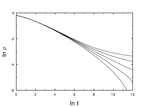
Figure 10: CP on a random hierarchical tree: activity versus time for $\lambda=2.73$, $2.74$, …, $2.77$ (lower to upper); system size: $N=262144$. Power-law decay is evident only for $\lambda=2.75$, close to the estimate $\lambda_{c}=2.76$ derived from QS simulations. Each curve represents an average over $100$ realizations; all realizations are performed on the same network.

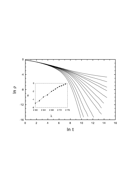
Figure 11: CP on a random hierarchical trees: activity versus time for $\lambda=2.60$, $2.62$, $2.64$, $2.68$, $2.69$, …, $2.75$ (lower to upper); system size $N=262144$. Each curve represents an average over $10^{3}$ - $10^{4}$ realizations, each performed on a different network. Inset: decay exponent $-\alpha$ versus $\lambda$.

Threshold model simulations

Threshold models represent an attempt to capture the activation threshold of real neurons, by requiring at least $m$ active neighbors associated with incoming links to activate a node with probability $\lambda$. In case of active nodes spontanous deactivation occurs with probability $\nu$ written in the reaction-diffusion model notation as:

(a)

$mA\to(m+1)A$ with probability $\lambda$,

(b)

$A\to\emptyset$ with probability $\nu$.

We use SCA updating, as in [39]. Since there is no spatial anisotropy (which might generate activity currents), we can assume that the SCA follow the same asymptotic dynamics as the corresponding model with random sequential updating. Thanks to the synchronous updates, we can speed up the simulations by $\sim n_{p}$ times by distributing the nodes among $n_{p}$ multiprocessor cores; by swapping the random number generation on parallel running graphics cards we obtain a further reduction of $50\%$ decrease in the simulation times. The spatio-temporal evolution of the HMN2d network with $m=6$, in a single network realization, starting from a fully active state, is shown in Figure 12. After a sharp initial drop in activity, due to spontaneous deactivation of nodes with few neighbors, one observes domains (modules) on which activity survives for a long time, suggesting rare region effects.

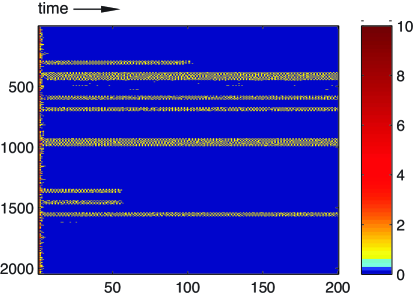
Figure 12: Spatio-temporal evolution of the density of the $m=6$ threshold model, proportional to the color coding on the right. The simulation is started from an active state, with $\nu=0.9$ and $\lambda=1$.

Results for threshold models

We begin by discussing the $m=2$ case, for which extensive simulations are performed. We generate networks with average degree $\langle k\rangle=24$ and $s=6$. Note that in this case values of $\langle k\rangle$ higher than the percolation threshold are needed to avoid modules having separated activities. As before, we averaged over hundreds of independent random networks and thousands of independent realizations. We followed the density up to $t_{max}=10^{5}$ MCs, starting from a fully active initial condition.

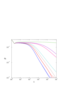
Figure 13: Decay of activity in the $m=2$ threshold model with $s=6$, and $\langle k\rangle=24$. The curves correspond to branching rates: $\lambda=0.65,0.66,0.67,0.68,0.83$ (lower to upper) and $\nu=0.7$ fixed. Levels: $l_{max}=8,9$ (thin, thick lines). Size-independent power-laws, reflecting a GP are observed.

In this case the mean activity density decays more rapidly than in mean-field theory, and is size-independent (see Figure 13). For large branching probabilities, $\langle\rho(t)\rangle$ seems to take a constant value, suggesting an active steady state, but at late times some deviation is observed, possibly due to finite-size effects.

Homogeneous triplet creation models (i.e., $m=3$) are expected to exhibit a mean-field-like discontinuous phase transition in two or more dimensions(see for example [54]). Disorder induces rounding effects, producing continuous phase transitions or GPs [55, 25]. We study a threshold model with $m=3$ and $s=6$, using $\langle k\rangle=36$. Our results are similar to those for $m=2$: non-universal power-laws, again suggesting a GP.

Quenched Mean-field approximation for SIS

Heterogeneous mean-field theory provides a good description of network models when fluctuations are irrelevant. This approximation is attractive because is can be solved analytically in many cases; the results agree with simulation [56, 57]. This analysis treats nodes with different degrees as distinct, but finally averages over all degree values, providing a homogeneous solution for the order parameter. To describe the effects of quasi-static heterogeneities in a more precise way, the so-called Quenched Mean-Field (QMF) approximation was introduced [58, 59]. For SIS models this leads to a spectral analysis of the adjacency matrix $A_{ij}$ of the network. The susceptible-infected-susceptible (SIS) [60] model is similar to the CP, except that branching rates are not normalized by $k$, leading to symmetric governing equations. A rate equation for the SIS model can be set up for the vector of activity probabilities $\rho_{i}(t)$ of node $i$ at time $t$:

$$\frac{d\rho_{i}(t)}{dt}=-\rho_{i}(t)+\lambda(1-\rho_{i}(t))\sum_{j=1}^{N}A_{ij}w_{ij}\rho_{j}(t)\leavevmode\nobreak\ .$$ (6)

Here the $w_{ij}=w_{ji}$ are weights attributed to the edges. For large times the SIS model evolves to a steady state, with an order parameter $\rho\equiv\langle{\rho_{i}}\rangle$. Since this equation is symmetric under the exchange $i\leftrightarrow j$, a spectral decomposition can be performed on a basis of orthonormal eigenvectors $\mbox{\boldmath$e$}(y)$.

$$\rho_{i}=\sum_{\Lambda}c(\Lambda)e_{i}(\Lambda).$$ (7)

Non-negativity of the matrix $B_{ij}\equiv A_{ij}w_{ij}$ assures a unique, real, non-negative largest eigenvalue $y_{M}$.

In the long-time limit the system evolves into a steady state and we can express the solution via $B_{ij}$ as

$$\rho_{i}=\frac{\lambda\sum_{j}B_{ij}\rho_{j}}{1+\lambda\sum_{j}B_{ij}\rho_{j}}\ .$$ (8)

Stability analysis shows that $\rho_{i}>0$ above a threshold $\lambda_{c}$, with an order parameter $\rho\equiv\langle{\rho_{i}}\rangle$. In the eigenvector basis equation (8) can be expanded by the coefficients $c(\Lambda)$ as

$$c(\Lambda)=\lambda\sum_{\Lambda^{\prime}}\Lambda^{\prime}c(\Lambda^{\prime})\sum_{i=1}^{N}\frac{e_{i}(\Lambda)e_{i}(\Lambda^{\prime})}{1+\lambda\sum_{\widetilde{\Lambda}}\widetilde{\Lambda}c(\widetilde{\Lambda})e_{i}(\widetilde{\Lambda})}$$ (9)

and near the threshold we can express $\rho_{i}\sim c_{i}(\Lambda_{1})e_{i}(\Lambda_{1})$ with the principal eigenvector. In the QMF approximation $1/\lambda_{c}=y_{1}$ and the order parameter can be approximated by the eigenvectors of the largest eigenvalues

$$\rho(\lambda)\approx a_{1}\Delta+a_{2}\Delta^{2}+...\ ,$$ (10)

where $\Delta=\lambda\Lambda_{1}{-}1{\ll}1$ with the coefficients

$$a_{j}=\sum_{i=1}^{N}e_{i}(\Lambda_{j})/[N\sum_{i=1}^{N}e_{i}^{3}(\Lambda_{j})].$$ (11)

As proposed in [59], and tested on several SIS network models [17], localization in the active steady state can be quantified by calculating the inverse participation ratio (IPR) of the principal eigenvector, related to the eigenvector of the largest eigenvalue $\mbox{\boldmath$e$}(y_{1})$ of the adjacency matrix as

$$I(N)\equiv\sum_{i=1}^{N}e_{i}^{4}(y_{1})\ .$$ (12)

This quantity vanishes $\sim 1/N$ in the case of homogeneous eigenvector components, but remains finite as $N\to\infty$ if activity is concentrated on a finite number of nodes. Numerical evidence has also been provided for the relation of localization to RR effects, slowing down the dynamics to follow power-laws [17].

We study localization of the SIS in the HMN2d models introduced in the previous section*s. We analyze the eigenvectors of $B_{ij}$ for $b=2$ ($\langle k\rangle\simeq 4$), varying $s$, using system sizes ranging from $N=256$ to $N=262144$. In particular, we performed a FSS scaling study of the IPR in these systems. First we determined the behavior on the small world network of [39] corresponding to $s=3/2$. As one can see in Figure 14, the localization at small sizes disappears as $I(N)\sim 1/N^{3}$. By contrast, for $s=3$ and $s=4$, the graphs are finite-dimensional, and the IPR increases with $N$, tending to a finite limiting value, suggesting localization.

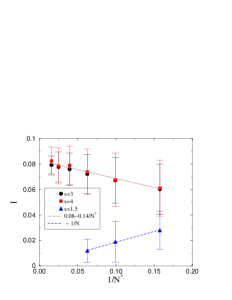
Figure 14: Finite size scaling of the inverse participation ratio in weakly coupled HMN2d models, with maximum levels $l_{max}=4,5,..9$. The $s=3$ (bullets) and $s=4$ (boxes) results suggest localization (finite $I$) in the infinite-size limit. Lines are power-law fits to the data. For $s=1.5$, corresponding to the symmetrized, small-world network (model-6 of [39]) no evidence of localization is seen.

One might question the relevance of network models with small connectivity to mammalian brains, in which $\langle k\rangle$ is on the order of $10^{3}$. To answer this we study $s\leq 4$ models with higher connectivity, i.e., $\langle k\rangle\simeq 50$. As Figure 15 shows, the sign of localization, which is weak but nonzero for $\langle k\rangle=4$, now disappears. Next, we add random weights $w_{ij}$, distributed uniformly over the interval $(0,1)$, to the links of the networks. A consequence of this explicit disorder is localization even in highly connected networks, as shown in Figure 15. This result is in agreement with the expectation of limited sustained activity in brain networks [39], meaning that the link disorder prevents over-excitation of a network of high connectivity.

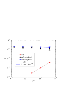
Figure 15: Finite size scaling of the inverse participation ratio in HMN2d models with higher average degree ($\langle k\rangle\simeq 50$) for maximum levels: $l_{max}=4,5,6,7,8$. Bullets: $s=3$ with uniform randomly distributed weights; boxes: without weights. Diamonds: $s=4$ with randomly distributed weights. Lines show power-law fits to the data. In the unweighted case, no localization effect can be seen, and $I$ decays linearly with $N$.

Localization suggests rare-region effects, thus a dynamic GP. Nevertheless, simulations of the CP on such networks do not show extended regions of power-laws for $s\leq 4$, but rather a nontrivial (non-mean-field) continuous phase transition (Figure 16). Decay simulations for $l=9$ yield $\rho(t)\simeq t^{-0.50(1)}$ at $\lambda_{c}\simeq 2.588(1)$, albeit with a cutoff due to the finite system size. This agrees with our result for 1D BB networks with $s=3$ [15]. Spreading simulations starting from single, randomly placed seed result in the survival probability scaling at this critical point: $P(t)\simeq t^{-0.50(1)}$ (that is, the symmetry $\alpha=\delta$ holds to within uncertainty). Here the density increases initially as $\rho(t)\simeq t^{0.23(1)}$. One can understand these results, noting that the localization values are rather small, $I\sim 0.08$, so that RR effects are too weak to generate observable GP effects in the dynamics.

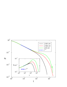
Figure 16: Evolution of the activity in the weighted CP on HMN2d networks with $s=4$, $l=9$, and $k=\langle 50\rangle$, for $\lambda=2.585$, $2.588$, and $2.59$ (lower to upper). Main plot: decay in case of a fully active initial state. Inset: growth of activity starting from a single active node for the same values of $\lambda$. Dashed lines are power-law fits for $\lambda_{c}\simeq 2.588$.

Naturally, for $s>4$ networks, where already the topological disorder is strong enough to create a GP, inhomogeneities in the interaction strengths amplify the RR effects. This induces GPs even for larger values of $\langle k\rangle$, as well as in the threshold models. Further studies of disorder effects are under way.

Conclusions

We investigate the dynamical behavior of spreading models on hierarchical modular networks embedded in two-dimensional space, with long links whose probability decays as a power-law with distance. This corresponds to an exponentially decreasing connection probability, as a function of the level in the hierarchical construction. The aim of this study is to understand the effects of intrinsic and topological disorder, in particular, extended critical regions in the parameter space, without any (self) tuning mechanism.

If we eliminate the underlying lattice structure we observe power-law dynamics for networks near the percolation threshold, when the effective dimension is finite. However, size-independent power-laws, corresponding to GPs, are only seen if we have directed links. Since connectivity of these structures is not guaranteed, we also study random hierarchical trees, with full connectivity. GPs are observed upon averaging over many independent network realizations. The relation to brain networks can be envisaged in the large-size limit, if we regard independent realizations as (almost decoupled) sub-modules of the entire brain.

When we ensure connectivity via short edges on the lowest level, we find GPs for rapidly decaying long-link probabilities. Both of these network assumptions are in accordance with empirical brain networks. Above the GP, at the critical point, we find mean-field-like decay of activity, in agreement with results on the CP with quenched disorder on higher-dimensional, regular lattices. We have also shown that bursty behavior arises naturally in the GPs, due to autocorrelations which decay via a power-law.

We perform a quenched mean-field study of the SIS model on these networks; in the SIS, nodes are connected symmetrically. Finite size scaling of the inverse participation ratio suggests localization on large-world networks and de-localization on small world structures. However, when we add intrinsic weight disorder, localization can be seen even on small-world networks. Weight disorder is again to be expected in real brain networks, since the strength of couplings varies over many orders of magnitude. Despite this, we saw no GP effects in the dynamics of weighted CPs with $s=4$. Instead, we find a nontrivial critical scaling, as has already been observed in other networks. The possibility of a narrow GP in this case is an open issue.

In conclusion, we believe our synthetic HMN2ds are closer to experimental brain networks than previously proposed models, and find numerical evidence for GPs in extended phases in simple models with spreading dynamics. Although we eliminate any self-tuning mechanisms, we still find nontrivial slow dynamics as well as localization of activity, which is crucial for understanding real brain network data.

Author contributions statement

Géza Ó. wrote, ran and analysed the CP and SIS simulations on HMN2d-s and performed the QMF analysis. R. D. wrote, ran and analyzed the HMT simulations. Gergely Ó. wrote and ran the HMN2 threshold model simulations and dimension measurements on them. Géza Ó. and R. D. wrote the main manuscript text. Géza Ó. prepared figures 1-3, 6-9, 13-16, R. D. prepared figures 4,5,10,11,17-20. Gergely Ó. prepared figure 12. All authors reviewed the manuscript.

Additional information

The authors declare no competing financial interests.

Supplementary information

Although the set of nodes is isomorphic to a square lattice of $N=2^{L}\!\times 2^{L}$ sites, we shall label the nodes not by their Cartesian coordinates but rather using a base-4 notation. At level $l$, the full set of $4^{l}$ nodes is divided into four quadrants labeled 0, 1, 2, and 3, proceeding counterclockwise from the lower left. At level $l-1$, each of the quadrants is similarly divided into four subquadrants, labeled in the same manner. Division into subquadrants continues all the way down to level 1, in which the elements are individual nodes. A given site can be specified by the labels of the quadrant, subquadrant, etc. to which it belongs. Denoting the labels at levels 1, 2,…, L, by $g_{1},...,g_{L}$, the address of a site is $n=\sum_{l=1}^{L}g_{l}\,4^{l-1}$ (see Fig. S17).

Figure 17: Definition of node labels for a network with $L=2$

Consider a set of four nodes, 0, 1, 2, and 3. There are six possible links between them: (0,1), (0,2), (0,3), (1,2), (1,3), and (2,3). A tree with four nodes has exactly three links. Of the $\binom{6}{3}=20$ subsets of three links, sixteen yield a connected tree [for example: {(0,1), (1,2), (2,3)}], while four correspond to a cycle of three nodes, leaving the fourth node isolated [example: {(1,2), (1,3), (2,3)}]. To construct a tree of four nodes, we choose one of the sixteen link sets ${\cal B}_{i}$ at random.

A hierarchical tree is constructed by first linking the four quadrants via three edges. The link set ${\cal B}_{i}$ is chosen at random. Then, for each link, we choose sites at random within each of the two quadrants connected by the link, to serve as the connected nodes. Now we repeat this process within each of the subquadrants, and so on, until we reach the basic modules of four sites. The latter are again connected by sets of three links, chosen independently from the basic collection of sixteen link sets. At the end, each basic module is connected internally, and to a module at the next level, etc., so that we have a connected graph of $N$ nodes and $N-1$ edges. Although we have chosen to begin the construction at level $L$, we could equally have begun at level 1, or some intermediate level: the choices of link sets and nodes at the various levels are mutually independent. These steps are illustrated in the Figs. S18, S19, S20.

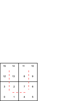
Figure 18: First step in constructing a network with $L=2$: define the link set at level 2.

Figure 19: Second step: choose nodes consistent with link set at level 2. At the next step (not shown) we choose link sets for each of the four-site modules.

Figure 20: Final step: choose nodes at level 1 consistent with the corresponding link sets.

At level 1 the number of links per node is 3/4; at level $j$, there are $4^{L-j}$ blocks connected via $4^{L-j}-1$ links. The number of links per node at this level is therefore $(4^{L-j}-1)/4^{L}\simeq 1/4^{j}$. Let $p_{j}$ denote the probability that a randomly chosen edge linking blocks at level $j$ be present. At level 1, links connect nodes within four-site modules. Since there are six possible links, and since just three are present within each module, we have $p_{1}=1/2$. At level 2, a link connects nodes within a 16-node module; at this level a node is linked to one of the 12 nodes outside its basic 4-site module. There are $(16\cdot 12)/2=96$ possible links, and since only three are present, $p_{2}=1/32$. At level $j$, an edge links nodes within a module containing $4^{j}$ nodes. The number of possible links at this level is $4^{j}(3\cdot 4^{j-1})/2$, so that $p_{j}=1/2^{4j-3}$, and, in general, $p_{j}/p_{j-1}=1/16$. Since a tree represents a minimally connected structure, $p_{j}$ cannot decay faster than this rate, in any connected hierarchical network based on four-node modules.

Although our principal interest is in random trees, as described above, we may also consider regular trees; these are constructed by using the same link set at each level. The resulting structure turns out to have infinite topological dimension, as discussed in Section ”Dimension measurements”.

References

- [1] Legenstein R. and Maass W., New Directions in Statistical Signal Processing: From Systems to Brain (eds S. Haykin, J. C. Principe, T. Sejnowski, J. McWhirter) 127 V154 (MIT Press, 2008).
- [2] Beggs J. and Plenz D., Neuronal avalanches in neocortical circuits. J. Neurosci. 23, 11167-11177 (2003).
- [3] Tetzlaff C, Okujeni S, Egert U, Wörgötter F, Butz M, Self-Organized Criticality in Developing Neuronal Networks. PLoS Comput. Biol. 6, e1001013 (2010).
- [4] Hahn G et al., Neuronal avalanches in spontaneous activity in vivo. J. Neurophysiol. 104, 3312-3322 (2010).
- [5] Ribieiro T. L. et al., Spike Avalanches Exhibit Universal Dynamics across the Sleep-Wake Cycle. PLoS ONE 5, e14129 (2010).
- [6] Bédard C, Kröger H., and Destexhe A, Does the 1/f Frequency Scaling of Brain Signals Reflect Self-Organized Critical States? Phys. Rev. Lett. 97, 118102 (2006).
- [7] Dehghani N et al., Avalanche Analysis from Multielectrode Ensemble Recordings in Cat, Monkey, and Human Cerebral Cortex during Wakefulness and Sleep. Front. Physiol. 3, 302 (2012).
- [8] Priesemann V, Valderrama M, Wibral M and Le Van Quyen M., Neuronal Avalanches Differ from Wakefulness to Deep Sleep VEvidence from Intracranial Depth Recordings in Humans. PLoS Comput. Biol. 9, e100298 (2014).
- [9] Beggs J. M. and Timme N., Being Critical of Criticality in the Brain. Front. Physiol. 3, 163 (2012).
- [10] Bak P., Tang C. and Wiesenfeld K., Self-organized criticality. Phys. Rev. A 38, 364 V374 (1988).
- [11] Pruessner G., Self Organized Criticality, (Cambridge University Press, 2012).
- [12] Vojta T., Rare region effects at classical, quantum and nonequilibrium phase transitions J. Physics A: Math. and Gen. 39, R143-R205 (2006).
- [13] Griffiths R. B., Nonanalytic Behavior Above the Critical Point in a Random Ising Ferromagnet. Phys. Rev. Lett. 23, 17-19 (1969).
- [14] Ódor, G. Slow, bursty dynamics as a consequence of quenched network topologies. Phys. Rev. E 89, 042102 (2014).
- [15] Muñoz M. A., Juhász R., Castellano C., and Ódor G., Griffiths Phases on Complex Networks. Phys. Rev. Lett. 105, 128701 (2010).
- [16] Johnson S., Torres J. J., and Marro J., Robust Short-Term Memory without Synaptic Learning. PLoS ONE 8, e50276 (2013).
- [17] Ódor G., Spectral analysis and slow spreading dynamics on complex networks. Phys. Rev. E 88, 032109 (2013).
- [18] Newman M. E. J., Networks: An Introduction, (Oxford Univ. Press, 2010).
- [19] Sporns O, Chialvo D. R., Kaiser M. and Hilgetag C. C, Organization, development and function of complex brain networks. Trends Cogn. Sci. 8, 418 V425 (2004).
- [20] Sporns O., Networks Of The Brain, (MIT Press, 2010)
- [21] Kaiser M, A tutorial in connectome analysis: topological and spatial features of brain networks. NeuroImage 57, 892 V907 (2011).
- [22] Meunier D., Lambiotte R. and Bullmore E., Modular and hierarchically modular organization of brain networks. Front. Neurosci. 4, 200 (2010).
- [23] Hilgetag C.C., Burns G.A., O’Neill M.A., Scannell J.W., Young M.P. Anatomical connectivity defines the organization of clusters of cortical areas in the macaque monkey and the cat. Phil. Trans. R. Soc. Lond. B 355, 91-100 (2000).
- [24] Moretti P., Muñoz M. A., Griffiths phases and the stretching of criticality in brain networks Nat. Commun. 4, 2521 (2013).
- [25] Villa Martin P. M., Moretti P. and and Muñoz M. A., Rounding of abrupt phase transitions in brain networks. J. Stat. Mech. P01003 (2015).
- [26] Humpries M. D., Gurney K. and Prescott T.J., The brainstem reticular formation is a small-world, not scale-free, network. Proc. Biol. Sci. 273, 503 V511 (2006).
- [27] Yu S., Huang D., Singer W., Nikolic D., A Small World of Neuronal Synchrony. Cereb. Cortex 18, 2891 V2901 (2008).
- [28] Rosenblum M. G., Pikovsky A. and Kurths J., Synchronization V A Universal Concept In Nonlinear Sciences (Cambridge University Press, 2001).
- [29] Kuramoto Y., Self-entrainment of a population of coupled non-linear oscillators. Lect. Notes Phys. 39, 420-422 (1975).
- [30] Villegas P., Moretti P., Muñoz M. A., Frustrated hierarchical synchronization and emergent complexity in the human connectome network. Sci. Rep. 4, 5990 (2014).
- [31] Ravasz E. and Barabási A., Hierarchical organization in complex networks., Phys. Rev. E 67, 026112 (2003).
- [32] Ódor G. and Pastor-Satorras R., Slow dynamics and rare-region effects in the contact process on weighted tree networks. Phys. Rev. E 86, 026117 (2012).
- [33] Felleman D. J. and Van Essen D. C., Distributed hierarchical processing in the primate cerebral cortex. Cereb. Cortex 1, 1-47 (1991).
- [34] Markov N. T. et al., Weight consistency specifies regularities of macaque cortical networks. Cereb. Cortex 21, 1254-72 (2010).
- [35] Granovetter M. S., The strength of weak ties. Am. J. Sociol. 78, 1360-1380 (1973).
- [36] Flake G. W., Lawrence S., and Giles C.L., Efficient identification of web commnunities Proceedings of the Sixth International Conference on Knowledge Discovery and Data Mining [150-160] (ACM, Boston, MA 2000).
- [37] Ravasz E., Somera A. L., Mongru D. A., Oltvai Z. N. and Barabási A.-L., Hierarchical organization of modularity in metabolic networks. Science 297, 1551-1555 (2002).
- [38] Vazquez A., Pastor-Satorras R. and Vespignani A., Large-scale topological and dynamical properties of the Internet. Phys. Rev. E 65, 066130 (2002).
- [39] Kaiser M. and Hilgetag C. C., Optimal hierarchical modular topologies for producing limited sustained activation of neural networks. Front. in Neuroinform. 4, 8 (2010).
- [40] Latham P. E. and Nirenberg S., Synergy, Redundancy, and Independence in Population Codes, Revisited. Neural Comp. 16,, 1385-1412 (2004).
- [41] Marro J. and Dickman R., Nonequilibrium Phase Transitions in Lattice Models, (Cambridge University Press, Cambridge, 1999).
- [42] Ódor, G., Universality classes in nonequilibrium lattice systems. Rev. Mod. Phys. 76, 663-724 (2004).
- [43] Ódor G., Universality in Nonequilibrium Lattice Systems, (World Scientific, Singapore, 2008).
- [44] Kaiser M., Hilgetag C. C. and van Ooyen A., A simple rule for axon outgrowth and synaptic competition generates realistic connection lengths and filling fractions. Cereb. Cortex 19, 3001-3010 (2009).
- [45] Benjamini I. and Berger N.,The diameter of long-range percolation clusters on finite cycles. Rand. Struct. Alg. 19, 102-111 (2001).
- [46] Harris T. E., Contact Interactions on a Lattice, Ann. Prob. 2, 969-988 (1974).
- [47] Liggett T. M., Interacting Particle Systems, (Springer-Verlag, 1985, Berlin).
- [48] Pastor-Satorras R. and Vespignani A., Evolution and Structure of the Internet: A Statistical Physics Approach (Cambridge University Press, Cambridge, 2004).
- [49] van Ballegooijen W. M. and Boerlijst M. C., Emergent trade-offs and selection for outbreak frequency in spatial epidemics. PNAS. USA 101, 18246-18250 (2004).
- [50] Sun G.-Q. et al., Influence of infection rate and migration on extinction of disease in spatial epidemics. J. of Theor. Bio. 264, 95-103 (2010).
- [51] Sun G.-Q. et al., Phase transition in spatial epidemics using cellular automata with noise. Ecol. Res. 26, 333-340 (2011).
- [52] Vojta T., Igo J., Hoyos J. A., Rare regions and Griffiths singularities at a clean critical point: The five-dimensional disordered contact process. Phys. Rev. E 90, 012139 (2014).
- [53] Oliveira M. M. and Dickman R., How to simulate the quasistationary state Phys. Rev. E 71, 016129 (2005).
- [54] Ódor, G. Phase transition classes in triplet and quadruplet reaction-diffusion models. Phys. Rev. E 67, 056114 (2003).
- [55] V. Martin P. M., Bonachela J. A. and Muñoz M.A., Quenched disorder forbids discontinuous transitions in nonequilibrium low-dimensional systems. Phys. Rev. E 89, 012145 (2014).
- [56] Boguñá M., Castellano C., and Pastor-Satorras R., Langevin approach for the dynamics of the contact process on annealed scale-free networks. Phys. Rev. E 79, 036110 (2009).
- [57] Mata A. S., Ferreira R. S., Ferreira S. C., Heterogeneous pair-approximation for the contact process on complex networks. New J. Phys. 16, 053006 (2014).
- [58] Chakrabarti D., Wang Y., Wang C., Leskovec J., and Faloutsos C., Epidemic thresholds in real networks. ACM Trans. Inf. Syst. Secur. 10, 1-26 (2008).
- [59] Goltsev A. V., Dorogovtsev S. N., Oliveira J. G., and Mendes J. F. F., Localization and Spreading of Diseases in Complex Networks. Phys. Rev. Lett. 109, 128702 (2012).
- [60] Bailey N. T. J., The Mathematical Theory of Infectious Diseases 2nd ed. (Griffin, London, 1975).