Emulating the CFHTLenS Weak Lensing data: Cosmological Constraints from moments and Minkowski functionals

Abstract

Weak gravitational lensing is a powerful cosmological probe, with non–Gaussian features potentially containing the majority of the information. We examine constraints on the parameter triplet $(\Omega_{m},w,\sigma_{8})$ from non-Gaussian features of the weak lensing convergence field, including a set of moments (up to $4^{\rm th}$ order) and Minkowski functionals, using publicly available data from the 154 deg² CFHTLenS survey. We utilize a suite of ray–tracing N-body simulations spanning 91 points in $(\Omega_{m},w,\sigma_{8})$ parameter space, replicating the galaxy sky positions, redshifts and shape noise in the CFHTLenS catalogs. We then build an emulator that interpolates the simulated descriptors as a function of $(\Omega_{m},w,\sigma_{8})$, and use it to compute the likelihood function and parameter constraints. We employ a principal component analysis to reduce dimensionality and to help stabilize the constraints with respect to the number of bins used to construct each statistic. Using the full set of statistics, we find $\Sigma_{8}\equiv\sigma_{8}(\Omega_{m}/0.27)^{0.55}=0.75\pm 0.04$ (68% C.L.), in agreement with previous values. We find that constraints on the $(\Omega_{m},\sigma_{8})$ doublet from the Minkowski functionals suffer a strong bias. However, high-order moments break the $(\Omega_{m},\sigma_{8})$ degeneracy and provide a tight constraint on these parameters with no apparent bias. The main contribution comes from quartic moments of derivatives.

I Introduction

Weak gravitational lensing (hereafter WL) is emerging as a promising technique to constrain cosmology. Techniques have been developed to construct cosmic shear fields with shape measurements in large galaxy catalogues. Although the shear two–point function (2PCF) is the most widely studied cosmological probe (see, e.g. (Kilbinger et al., 2013)), alternative statistics have been shown to increase the amount of cosmological information one can extract from weak lensing fields. Among these, high–order moments ((Bernardeau et al., 1997; Hui, 1999; Van Waerbeke et al., 2001; Takada and Jain, 2002; Kilbinger and Schneider, 2005)), three–point functions ((Schneider and Lombardi, 2003; Takada and Jain, 2003; Zaldarriaga and Scoccimarro, 2003)), bispectra ((Takada and Jain, 2004; Dodelson and Zhang, 2005; Sefusatti et al., 2006; Bergé et al., 2010)), peak counts ((Jain and Van Waerbeke, 2000; Marian et al., 2009; Maturi et al., 2010; Yang et al., 2011; Marian et al., 2013; Bard et al., 2013; Dietrich and Hartlap, 2010; Lin and Kilbinger, 2015)) and Minkowski Functionals ((Kratochvil et al., 2012; Petri et al., 2013)) have been shown to improve cosmological constraints in weak lensing analyses.

In this work, we use the publicly available CFHTLenS data, consisting of a catalog of $\approx$4.2 million galaxies, combined with a suite of ray-tracing simulations in 91 different cosmological models to derive constraints on the cosmological parameters $\Omega_{m}$, $\sigma_{8}$ and the dark energy (DE) equation of state $w$. The statistics we consider in this work are the Minkowski functionals (MFs) and the low–order moments (LM) of the convergence field. Cosmological parameter inferences from CFHTLenS have been obtained using the 2PCF (Kilbinger et al., 2013), and a number of authors have investigated the constraining power of CFHTLenS using statistics that go beyond the usual quadratic ones. Fu et al. (Fu et al., 2014) used three–point correlations as an additional probe for cosmology, and found modest ($10-20\%$) improvements over the 2PCF. These results rely on the third order statistics systematic tests performed by Simon et al. (Simon et al., 2015).

Liu et al. (Liu et al., 2014a) have found a more significant ($50-60\%$) tightening of the $\Omega$ and $\sigma_{8}$ constraints, utilizing the abundance of WL peaks. Cosmological constraints using WL peaks in CFHTLenS Stripe82 data have also been investigated by Liu et. al. (Liu et al., 2014b). Finally, closest to the present paper, Shirasaki & Yoshida (Shirasaki and Yoshida, 2014) investigated constraints from Minkowski Functionals, including systematic errors. Our study represents two major improvements over previous work. First, constraints from the MFs in ref. (Shirasaki and Yoshida, 2014) were obtained through the Fisher matrix formalism, assuming linear dependence on cosmological parameters. Our study utilizes a suite of simulations sampling the cosmological parameter space, mapping out the non-linear parameter-dependence of each descriptor. Second, we include the LMs as a set of new descriptors; these yield the tightest and least biased constraints.

This paper is organized as follows: we first give an overview of the CFHTLenS catalogs, and summarize the adopted data reduction techniques. Next, we give a description of our simulation pipeline, including the ray–tracing algorithm, and the procedure used to sample the parameter space. We call the statistical weak lensing observables – the power spectrum, Minkowski functionals, and moments – ”descriptors” throughout the paper. We discuss the calculation of the descriptors, including dimensional reduction using a principal component analysis, and the statistical inference framework we used. We then describe our main results, i.e. the cosmological parameter constraints. To conclude, we then discuss our findings and comment on possible future extensions of this analysis.

II Data and simulations

II.1 CFHTLenS data reduction

In this section, we briefly summarize our treatment of the public CFHTLenS data. For a more in–depth description of our data reduction procedure, we refer the reader to (Liu et al., 2014a).

The CFHTLenS survey covers four sky patches of 64, 23, 44 and 23 deg² area, for a total of 154 deg². The publicly released data consist of a galaxy catalog created using SExtractor (Erben et al., 2013), and includes photometric redshifts estimated with a Bayesian photometric redshift code (Hildebrandt et al., 2012) and galaxy shape measurements using lensfit (Heymans et al., 2012; Miller et al., 2013).

We apply the following cuts to the galaxy catalog: mask $<1$ (see Table B2 in (Erben et al., 2013)), redshift $0.2<z<1.3$ (see (Heymans et al., 2012)), fitclass = 0 (which requires the object to be a galaxy) and weight $\mathrm{w}>0$ (with larger $\mathrm{w}$ indicating smaller shear measurement uncertainty). Applying these cuts leaves us 4.2$\times 10^{6}$ galaxies, 124.7 deg² sky coverage, and average galaxy density $n_{gal}\approx 9.3\,\mathrm{arcmin}^{-2}$. The catalog is further reduced by $\sim 25\%$ when one rejects fields with non–negligible star–galaxy correlations. These spurious correlations are likely due to imperfect PSF removal, and do not contain cosmological signal. These cuts are consistent with the ones adopted by the CFHTLenS collaboration (see (Fu et al., 2014)).

The CFHTLenS galaxy catalog provides us with the sky position $\boldsymbol{\theta}$, redshift $z(\boldsymbol{\theta})$ and ellipticity $\mathbf{e}(\boldsymbol{\theta})$ of each galaxy, as well as the individual weight factors $w(\boldsymbol{\theta})$ and additive and multiplicative ellipticity corrections $c(\boldsymbol{\theta}),m(\boldsymbol{\theta})$. Because the CFHTLenS fields are irregularly shaped, we first divide them into 13 squares (subfields) to match the shape and $\approx 12$ deg² size of our simulated maps (see below). These square-shaped subfield maps are pixelized according to a Gaussian gridding procedure

$$\bar{\mathbf{e}}(\boldsymbol{\theta})=\frac{\sum_{i=1}^{N_{s}}W(|\boldsymbol{\theta}-\boldsymbol{\theta}_{i}|)\mathrm{w}(\boldsymbol{\theta}_{i})[\mathbf{e}^{obs}(\boldsymbol{\theta}_{i})-c(\boldsymbol{\theta}_{i})]}{\sum_{i=1}^{N_{s}}W(|\boldsymbol{\theta}-\boldsymbol{\theta}_{i}|)\mathrm{w}(\boldsymbol{\theta}_{i})[1+m(\boldsymbol{\theta})]},$$ (1)

$$W_{\theta_{G}}(\boldsymbol{\theta})=\frac{1}{2\pi\theta_{G}^{2}}\exp{\left(-\frac{\boldsymbol{\theta}^{2}}{2\theta_{G}^{2}}\right)},$$ (2)

where the smoothing scale $\theta_{G}$ has been fixed at 1.0 arcmin (but varied occasionally to 1.8 and 3.5 arcmin for specific tests described below) and $m,c$ refer to the multiplicative and additive corrections of the galaxies in the catalog.

Using the ellipticity grid $\bar{\mathbf{e}}(\boldsymbol{\theta})$ as an estimator for the cosmic shear $\gamma^{1,2}(\boldsymbol{\theta})$, we perform a non–local Kaiser–Squires inversion (Kaiser and Squires, 1993) to recover the convergence $\kappa(\boldsymbol{\theta})$ from the $E$–mode of the shear field,

$$\kappa(\mathbf{l})=\left(\frac{l_{1}^{2}-l_{2}^{2}}{l_{1}^{2}+l_{2}^{2}}\right)\gamma^{1}(\mathbf{l})+2\frac{l_{1}l_{2}}{l_{1}^{2}+l_{2}^{2}}\gamma^{2}(\mathbf{l}).$$ (3)

The simulated $\kappa$ maps we create below are $12~{}\mathrm{deg}^{2}$ in size and have a resolution of $512\times 512$ pixels. The CFHTLenS catalogs contain masked regions (which include the rejected fields and the regions around bright stars). We first create gridded versions of the observed $\kappa$ maps matching the size and pixel resolution of our simulated maps, with each pixel containing the number of galaxies ($n_{gal}$) falling within its window. We then smooth this galaxy surface density map with the same Gaussian window function as equation (2) and remove regions where $n_{gal}<5\,\mathrm{arcmin}^{−2}$ (see (Shirasaki and Yoshida, 2014)). Regions with low galaxy number density can induce large errors in the cosmological parameter inferences.

II.2 Simulation design

We next give a description of our method to sample the parameter space with a suite of N–body simulations. We wish to investigate the non–linear dependence of the descriptors (in this work, Minkowski Functionals and moments of the $\kappa$ field) on the parameter triplet $\mathbf{p}=(\Omega_{m},w,\sigma_{8})$, while keeping the other relevant parameters $(h,\Omega_{b},n_{s})$ fixed to the values (0.7, 0.046, 0.96) (see (Hinshaw et al., 2013)). We sampled the $D$–dimensional ($D=3$ in this case) parameter space using an irregularly spaced grid. The grid was designed with a method similar to that used to construct an emulator for the matter power spectrum in the Coyote simulation suite (Heitmann et al., 2009). Given fixed available computing resources, the irregular grid design is more efficient than a parameter grid with regular spacings: to achieve the same average spacing between models in the latter approach would require a prohibitively large number of simulations.

We limit the parameter sampling to a box whose sides range over $\Omega_{m}\in[0.07,1],\,w\in[-3.0,0],\,\sigma_{8}\in[0.1,1.5]$. These are large ranges, with most of the corresponding 3D parameter volume ruled out by other cosmological experiments. However, our focus in this work is to quantify the constraints from CFHTLenS alone, which, by itself has strong parameter degeneracies. We next map this sampling box $\Pi$ into a hypercube of unit side. We want to construct an irregularly spaced grid consisting of $N$ points $\mathbf{x}_{i}\in[0,1]^{D}$. Let a design $\mathcal{D}$ be the set of this irregularly spaced $N$ points. Our goal is to find an optimal design, in which the points are spread as uniformly as possible inside the box. Following ref. (Heitmann et al., 2009), we choose our optimal design as the minimum of the cost function

$$\mathcal{C}(\mathcal{D})=\frac{2D^{1/2}}{N(N-1)}\sum_{i<j}^{N}\frac{1}{|\mathbf{x}_{i}-\mathbf{x}_{j}|}.$$ (4)

This problem is mathematically equivalent to the minimization of the Coulomb potential energy of $N$ unit charges in a unit box, which corresponds to spreading the charges as evenly as possible. Finding the optimal design $\mathcal{D}_{m}$ that minimizes (4) can be computationally very demanding, and hence we decided to use a simplified approach. Although approximate, the following iterative procedure gives satisfactory accuracy for our purposes:

1. We start from the diagonal design $\mathcal{D}_{0}$: $x_{i}^{d}\equiv i/(N-1)$ for $d=1...D$.

2. We shuffle the coordinates of the particles in each dimension independently $x_{i}^{d}=\mathcal{P}_{d}\left(\frac{1}{N-1},\frac{2}{N-1},...,1\right)$, where $\mathcal{P}_{1},...,\mathcal{P}_{D}$ are random independent permutations of $(1,2,...,N)$.

3. We pick a random particle pair $(i,j)$ and a random coordinate $d\in\{1,...,D\}$ and swap $x_{i}^{d}\leftrightarrow x_{j}^{d}$.

4. We compute the new cost function. If the value is less than in the previous step, we keep the exchange, otherwise we revert the coordinate swap.

5. We repeat steps 3 and 4 until the relative cost function change is less than a chosen accuracy parameter $\epsilon$.

We have found that for $N=91$ grid points O($10^{5}$) iterations are sufficient to reach an accuracy of $\epsilon\sim 10^{-4}$. Once the optimal design $\mathcal{D}_{m}$ has been determined, we invert the mapping $\Pi\rightarrow[0,1]^{3}$ to arrive at our simulation parameter sampling $\mathbf{p}_{s}$. We show the final list of grid points in Table 1 and Figure 1.

$N$	$\Omega_{m}$	$w$	$\sigma_{8}$	$N$	$\Omega_{m}$	$w$	$\sigma_{8}$	$N$	$\Omega_{m}$	$w$	$\sigma_{8}$	$N$	$\Omega_{m}$	$w$	$\sigma_{8}$
1	0.136	-2.484	1.034	26	0.380	-2.424	0.199	51	0.615	-1.668	0.185	76	0.849	-0.183	0.821
2	0.145	-2.211	1.303	27	0.389	-0.939	0.454	52	0.624	-2.757	0.327	77	0.859	-1.182	1.415
3	0.155	-0.393	0.652	28	0.399	-1.938	1.500	53	0.634	-1.575	0.976	78	0.869	-2.031	0.227
4	0.164	-2.181	0.313	29	0.409	-2.940	0.737	54	0.643	-2.454	1.444	79	0.878	-2.697	0.524
5	0.173	-0.423	1.231	30	0.418	-1.758	0.383	55	0.652	-1.029	1.458	80	0.887	-0.363	0.439
6	0.183	-0.909	0.269	31	0.427	-2.910	0.411	56	0.661	-0.486	0.892	81	0.897	-0.999	0.468
7	0.192	-1.605	1.401	32	0.436	-0.060	0.878	57	0.671	-2.364	0.793	82	0.906	-1.698	1.273
8	0.201	-2.787	0.807	33	0.446	-1.212	1.486	58	0.681	-2.970	0.610	83	0.915	-2.544	1.175
9	0.211	-0.333	0.341	34	0.455	-2.637	1.373	59	0.690	-1.332	0.482	84	0.925	-0.636	1.259
10	0.221	-1.485	0.666	35	0.464	-2.121	0.906	60	0.700	-0.273	0.283	85	0.943	-2.394	0.835
11	0.239	-1.848	0.962	36	0.474	-1.302	0.114	61	0.709	-2.061	0.425	86	0.953	-1.545	0.355
12	0.249	-2.727	0.369	37	0.483	-1.515	0.680	62	0.718	-1.728	1.472	87	0.963	-2.151	0.510
13	0.258	-1.395	0.241	38	0.493	-0.243	0.297	63	0.728	-0.120	0.596	88	0.972	-0.666	0.694
14	0.267	-2.667	1.317	39	0.502	-1.152	1.189	64	0.737	-2.847	1.203	89	0.981	-1.242	1.048
15	0.276	-0.849	1.429	40	0.512	-0.819	0.849	65	0.746	-0.090	1.118	90	0.991	-1.908	1.020
16	0.286	-1.272	1.104	41	0.521	-2.334	0.538	66	0.755	-0.456	1.359	91	1.000	-1.425	0.708
17	0.295	-1.878	0.100	42	0.530	0.000	0.624	67	0.765	-2.091	1.076	–	–	–	–
18	0.305	-0.879	0.765	43	0.540	-0.030	1.161	68	0.775	-1.122	1.132	–	–	–	–
19	0.315	-2.241	0.638	44	0.549	-1.818	1.287	69	0.784	-1.062	0.779	–	–	–	–
20	0.324	-2.001	1.217	45	0.558	-2.577	1.146	70	0.794	-1.365	0.156	–	–	–	–
21	0.333	-0.213	0.552	46	0.568	-0.516	1.331	71	0.803	-2.607	0.255	–	–	–	–
22	0.342	-2.817	1.062	47	0.577	-3.000	0.948	72	0.812	-1.788	0.722	–	–	–	–
23	0.352	-0.576	1.090	48	0.587	-2.304	0.128	73	0.821	-2.880	0.863	–	–	–	–
24	0.361	-0.606	0.171	49	0.596	-0.696	0.496	74	0.831	-0.759	0.213	–	–	–	–
25	0.370	-0.303	1.345	50	0.606	-0.789	0.142	75	0.840	-2.274	1.387	–	–	–	–

Table 1: List of the CFHTemu1 grid points in the 3D cosmological parameter space.

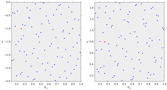
Figure 1: $(\Omega_{m},w)$ and $(\Omega_{m},\sigma_{8})$ projections of the final simulation design. The blue points correspond to the CFHTemu1 simulation set, which consists of one $N$–body simulation per point, while the red point corresponds to the CFHTcov simulation set, which is based on 50 independent $N$–body simulations.

For each parameter point on the grid $\mathbf{p}_{s}$ we then run an $N$–body simulation and perform ray tracing, as described in § II.3, to simulate CFHTLenS shear catalogs. Throughout the rest of this paper, we refer to this set of simulations as CFHTemu1. Additionally, we have run 50 independent $N$–body simulations with a fiducial parameter choice $\mathbf{p}_{0}=(0.26,-1.0,0.8)$, for the purpose of accurately measuring the covariance matrices, needed for the parameter inferences in §III.2. This additional suite of 50 simulations will be referred to as CFHTcov.

II.3 Ray–Tracing Simulations

The goal of this section is to outline our simulation pipeline. The fluctuations in the matter density field between a source at redshift $z$ and an observer located on Earth will cause small deflections in the trajectories of light rays traveling from the source to the observer. We estimate the dark matter gravitational potential running $N$–body simulations with $N=512^{3}$ particles, using the public code Gadget2 (Springel, 2005). We adopted a comoving box size of $240h^{-1}$Mpc, corresponding to a mass resolution of $7.4\times 10^{9}h^{-1}M_{\odot}$. The simulations include dark matter only, and the initial conditions were generated with N-GenIC at $z=100$, based on the linear matter power spectrum created with the Einstein-Boltzmann code CAMB Lewis et al. (2000). Data cubes were output at redshift intervals corresponding to $80h^{-1}$ (comoving) Mpc.

Using a procedure similar to refs. (Jain et al., 2000; Hilbert et al., 2009), the equation that governs the light ray deflections can be written in the form

$$\frac{d^{2}\mathbf{x}(\chi)}{d\chi^{2}}=-\frac{2}{c^{2}}\nabla_{\mathbf{x}_{\perp}}\Phi(\mathbf{x}_{\perp}(\chi),\chi),$$ (5)

where $\chi$ is the radial comoving distance, $\mathbf{x}_{\perp}=\chi\boldsymbol{\beta}$ refers to two transverse coordinates (with $\boldsymbol{\beta}$ the angular sky coordinates, using the flat sky approximation)a, $\mathbf{x}(\chi)$ is the trajectory of a single light ray, and $\Phi$ is the gravitational potential.

Suppose that a light ray reaches the observer at an angular position $\boldsymbol{\theta}$ on the sky: we want to know where this light ray originated, knowing it comes from a redshift $z_{s}$. To answer this question we need to integrate equation (5) with the initial condition $\boldsymbol{\beta}(0;\boldsymbol{\theta})=\boldsymbol{\theta}$ up to a distance $\chi_{s}=\chi(z_{s})$ to obtain the source angular position $\boldsymbol{\beta}(\chi_{s};\boldsymbol{\theta})$. Since light rays travel undeflected from the observer to the first lens plane, the derivative initial condition in the Cauchy problem (5) reads $\dot{\boldsymbol{\beta}}(0;\boldsymbol{\theta})=0$. We indicate the derivative of $\boldsymbol{\beta}$ with respect to $\chi$ as $\dot{\boldsymbol{\beta}}$. We use our proprietary implementation Inspector Gadget (see, e.g., Kratochvil et al. (2010)) to solve for the light ray trajectories based on a discretized version of equation (5) that is based on the multi–lens–plane algorithm (see (Hilbert et al., 2009) for example). Applying random periodical shifts and rotations to the $N$–body simulation data cubes, we generate $R=1000$ pseudo–independent realizations of the lens plane system used to solve (5). Once we obtain the light ray trajectories, we infer the relevant weak lensing quantities by taking angular derivatives of the ray deflections $A(\chi_{s};\boldsymbol{\theta})=\partial\boldsymbol{\beta}(\chi_{s};\boldsymbol{\theta})/\partial\boldsymbol{\theta}$ and performing the usual spin decomposition to infer the convergence $\kappa$ and the shear components $(\gamma^{1},\gamma^{2})$,

$$A(\chi_{s};\boldsymbol{\theta})=(1-\kappa(\chi_{s};\boldsymbol{\theta}))\boldsymbol{I}-\gamma^{1}(\chi_{s};\boldsymbol{\theta})\sigma^{3}-\gamma^{2}(\chi_{s};\boldsymbol{\theta})\sigma^{1}$$ (6)

where $\boldsymbol{I}$ is the $2\times 2$ identity and $\sigma^{1,3}$ are the first and third Pauli matrices. We perform this procedure for each of the $R$ realizations of the lens planes and we obtain $R$ pseudo–independent realizations of the $\boldsymbol{\gamma}$ weak lensing field. We use these different random realizations to estimate the means (from the CFHTemu1 simulations) and covariance matrices (from the CFHTcov simulations) of our descriptors. Since the random box rotations and translations that make up the CFHTcov simulations are based on 50 independent $N$–body runs, we believe the covariance matrices measured from this set to be more accurate than the ones measured from the CFHTemu1 set.

The convergence $\kappa$ is related to the magnification, while the two components of the complex shear $\boldsymbol{\gamma}=\gamma^{1}+i\gamma^{2}$ are related to the apparent ellipticity of the source. Given a source with intrinsic complex ellipticity $\mathbf{e}_{s}=e^{1}_{s}+ie^{2}_{s}$, its observed ellipticity will be modified to

$$\mathbf{e}=\begin{cases}\frac{\mathbf{e}_{s}+\mathbf{g}}{1+\mathbf{g}^{*}\mathbf{e}_{s}}\,\,\,\,\,\,\,\,|\mathbf{g}|\leq 1\\ \\ \frac{1+\mathbf{ge}_{s}^{*}}{\mathbf{e}_{s}^{*}+\mathbf{g}^{*}}\,\,\,\,\,\,\,\,|\mathbf{g}|>1\end{cases}$$ (7)

where $\mathbf{g}\equiv\boldsymbol{\gamma}/(1-\kappa)$ is the reduced shear.

For each simulated galaxy, we assign an intrinsic ellipticity by rotating the observed ellipticity for that galaxy by a random angle on the sky, while conserving its magnitude $|\mathbf{e}|$. To be consistent with the CFHTLenS analysis, we adopt the weak lensing limit ($|\boldsymbol{\gamma}|\ll 1,\kappa\ll 1$), i.e. $\mathbf{g}\approx\boldsymbol{\gamma}$ and $\mathbf{e}\approx\mathbf{e}_{s}+\boldsymbol{\gamma}$. We also add the multiplicative shear corrections by replacing $\boldsymbol{\gamma}$ with $(1+m)\boldsymbol{\gamma}$. We note that the observed ellipticity for a particular galaxy already contains the lensing shear by large scale structure (LSS), but the random rotation makes this contribution at least second order in $\kappa$ by destroying the shape spatial correlations induced by lensing from LSS. Consistent with the weak lensing approximation, the lensing signal from the simulations is first order in $\kappa$ and hence the randomly rotated observed ellipticities can be safely considered as intrinsic ellipticities.

We analyze the simulations in the same way as we analyzed the CFHTLenS data – constructing the simulated $\kappa$ maps as explained in §II.1. These final simulation products are then processed together with the $\kappa$ maps obtained from the data to compute confidence intervals on the parameter triplet $(\Omega_{m},w,\sigma_{8})$.

III Statistical methods

The goal of this section is to describe the framework to combine the CFHT data and our simulations, and to derive the constraints on the cosmological parameter triplet $(\Omega_{m},w,\sigma_{8})$. Briefly, we measure the same set of statistical descriptors from the data and from the simulations; these are then compared in a Bayesian framework in order to compute parameter confidence intervals.

III.1 Descriptors

The statistical descriptors we consider in this work are the Minkowski Functionals (MFs) and the low–order moments (LMs) of the convergence field. The three MFs $(V_{0},V_{1},V_{2})$ are topological descriptors of the convergence field $\kappa(\boldsymbol{\theta})$, probing the area, perimeter and genus characteristic of the $\kappa$ excursion sets $\Sigma_{\kappa_{0}}$, defined as $\Sigma_{\kappa_{0}}=\{\kappa>\kappa_{0}\}$. Following refs. (Petri et al., 2013; Kratochvil et al., 2012) we use the following local estimators to measure the MFs from the $\kappa$ maps:

$$V_{0}(\kappa_{0})=\frac{1}{A}\int_{A}\Theta(\kappa(\boldsymbol{\theta})-\kappa_{0})d\boldsymbol{\theta},$$

$$V_{1}(\kappa_{0})=\frac{1}{4A}\int_{A}\delta_{D}(\kappa(\boldsymbol{\theta})-\kappa_{0})\sqrt{\kappa_{x}^{2}+\kappa_{y}^{2}}d\boldsymbol{\theta},$$ (8)

$$V_{2}(\kappa_{0})=\frac{1}{2\pi A}\int_{A}\delta_{D}(\kappa(\boldsymbol{\theta})-\kappa_{0})\frac{2\kappa_{x}\kappa_{y}\kappa_{xy}-\kappa_{x}^{2}\kappa_{yy}-\kappa_{y}^{2}\kappa_{xx}}{\kappa_{x}^{2}+\kappa_{y}^{2}}d\boldsymbol{\theta}.$$

Here $A$ is the total area of the field of view and $\kappa_{x,y}$ denotes gradients of the $\kappa$ field, which we evaluate using finite differences. In this notation $\Theta(x)$ is the Heaviside function and $\delta_{D}(x)$ is the Dirac delta function. The first Minkowski functional, $V_{0}$, is equivalent to the cumulative one–point PDF of the $\kappa$ field, while $V_{1},V_{2}$ are sensitive to the correlations between nearby pixels. The one–point PDF of the $\kappa$ field, $\partial V_{0}$, can be obtained by differentiation $\partial V_{0}(\kappa_{0})=dV_{0}(\kappa_{0})/d\kappa_{0}$.

In addition to these topological descriptors, we consider a set of low–order moments of the convergence field (two quadratic, three cubic and four quartic). We choose these moments to be the minimal set of LMs necessary to build a perturbative expansion of the MFs up to $O(\sigma_{0}^{2})$ (see (Munshi et al., 2012; Matsubara, 2010)). We adopt the following definitions

$$\begin{matrix}\mathrm{LM_{2}}:\sigma_{0,1}^{2}=\langle\kappa^{2}\rangle,\langle|\nabla\kappa|^{2}\rangle,\\ \\ \mathrm{LM_{3}}:S_{0,1,2}=\langle\kappa^{3}\rangle,\langle\kappa|\nabla\kappa|^{2}\rangle,\langle\kappa^{2}\nabla^{2}\kappa\rangle,\\ \\ \mathrm{LM_{4}}:K_{0,1,2,3}=\langle\kappa^{4}\rangle,\langle\kappa^{2}|\nabla\kappa|^{2}\rangle,\langle\kappa^{3}\nabla^{2}\kappa\rangle,\langle|\nabla\kappa|^{4}\rangle.\end{matrix}$$ (9)

If the $\kappa$ field were Gaussian, one could express the MFs in terms of the LM₂ moments, which are the only independent moments for a Gaussian random field. In reality, weak lensing convergence fields are non–Gaussian and the MF and LM descriptors are not guaranteed to be equivalent. Refs. (Munshi et al., 2012; Matsubara, 2010) studied a perturbative expansion of the MFs in powers of the standard deviation $\sigma_{0}$ of the $\kappa$ field. When truncated at order $O(\sigma_{0}^{2})$, this can be expressed completely in terms of the LMs up to quartic order. Such perturbative series, however, have been shown not to converge (Petri et al., 2013) unless the weak lensing fields are smoothed with windows of size $\geq 15^{\prime}$. Because of this, throughout this work, we treat MF and LM as separate statistical descriptors.

We note that this choice is somewhat ad-hoc. In general, the LMs that contain gradients are sensitive to different shapes of the $\kappa$ multispectra $P_{\kappa}^{n}(\mathbf{l}_{1},...,\mathbf{l}_{n})$ because a particular $\mathrm{LM}_{n}$ has the general form

$$\mathrm{LM}_{n}=\int d\mathbf{l}_{1}...d\mathbf{l}_{n}\rho(\mathbf{l}_{1...n})P^{n}_{\kappa}(\mathbf{l}_{1...n})$$ (10)

where $\rho$ is a polynomial of order $n$ in the $\mathbf{l}$’s. For example for $K_{2}$ we have $\rho(\mathbf{l}_{1234})=l_{4}^{2}$ and this moment emphasizes quadrilateral shapes for which one side is much larger than the others. On the other hand, for $K_{3}$ we have $\rho(\mathbf{l}_{1234})=(\mathbf{l}_{1}\cdot\mathbf{l}_{2})(\mathbf{l}_{3}\cdot\mathbf{l}_{4})$ and this moment is most sensitive to trispectrum shapes that are close to rectangular. There are moments which include derivatives in addition to those included in Eq. 9. In the future, we will investigate whether there is additional constraining power in these additional quartic moments.

In addition to the MFs and LMs, we consider the angular power spectrum $P_{l}\equiv P^{2}_{l}$ of $\kappa$, defined as

$$\langle\tilde{\kappa}(\mathbf{l})\tilde{\kappa}(\mathbf{l}^{\prime})\rangle=(2\pi)^{2}\delta_{D}(\mathbf{l}+\mathbf{l}^{\prime})P_{l},$$ (11)

where $\tilde{\kappa}(\mathbf{l})$ is the Fourier transform of the $\kappa$ field. Previous works have studied cosmological constraints from the convergence power spectrum extensively. Here our purpose is to compare the constraints we obtain from the MFs and LMs to ones present in the literature, which are based on the use of quadratic statistics (see for example (Kilbinger et al., 2013)). The statistical descriptors used in this work are summarized in Table 2.

Descriptor	Details	$N_{b}$ (linear spacing)
$V_{0},V_{1},V_{2}$ (MF)	$\kappa_{0}\in[-0.04,0.12]$	50
Power Spectrum (PS)	$l\in[300,5000]$	50
Moments (LM)	–	9

Table 2: Summary of the descriptors we used, together with the specifications and the number of bins $N_{b}$ in each case.

When measuring statistical descriptors on $\kappa$ maps, particular attention must be paid to the effect of masked pixels. The MFs and LMs remain well–defined in the presence of masks, since the estimators in equations (8) and (9) are defined locally, and can be computed in the non–masked regions (with the exception of the few pixels that are close to the mask boundaries). The situation is more complicated for power spectrum measurements, which require the evaluations of Fourier transforms and hence rely on the value of every pixel in the map. Although sophisticated schemes to interpolate over the masked regions have been studied (see for example (VanderPlas et al., 2012)), for the sake of simplicity, we here insert the value $\kappa=0$ in each masked pixel. Given the uniform spatial distribution of the masked regions in the data, we expect that masks have a little effect on the power spectrum at the range of multipoles in Table 2, except for an overall normalization which will be the same both in the data and the simulations. Likewise, we believe that the way we deal with masked sky regions – essentially ignoring them – is robust for the MFs and LMs. Since we apply the same masks to our simulations and the data, they are unlikely to introduce biases in the resulting constraints. Masks, of course, can still affect the sensitivity and weaken constraints. The impact of the masks and their treatment has been evaluated for the MFs, obtained from CFHTLenS, by ref. (Shirasaki and Yoshida, 2014), in which the authors find that the masked regions are not a dominant source of systematic effects in the CFHTLenS data.

III.2 Cosmological parameter inferences

In this section, we briefly outline the statistical framework adopted for computing cosmological parameter confidence levels. We make use of the MFs and LMs, as well as the power spectrum, as discussed in the previous section. We refer to $M_{i}^{r}(\mathbf{p})$ as the descriptor measured from a realization $r$ of one of our simulations with a choice of cosmological parameters $\mathbf{p}$ (i.e. from one of the $R=1000$ map realizations in this cosmology), and to $D_{i}$ as the descriptor measured from the CFHTLenS data. In this notation, $i$ is an index that refers to the particular bin on which the descriptor is evaluated (for example $i$ can range from 0 to 9 for the LM statistic and from 0 to $N_{b}-1$ for a MF measured in $N_{b}$ different, linearly spaced $\kappa$ bins, as indicated in Table 2).

Once we make an assumption for the data likelihood $\mathcal{L}_{d}(D_{i}|\mathbf{p})$ and for the parameter priors $\Pi(\mathbf{p})$, we can use Bayes’ theorem to compute the parameter likelihood $\mathcal{L}_{p}$,

$$\mathcal{L}_{p}(\mathbf{p}|D_{i})=\frac{\mathcal{L}_{d}(D_{i}|\mathbf{p})\Pi(\mathbf{p})}{N_{\mathcal{L}}}.$$ (12)

Here $N_{\mathcal{L}}$ is a $\mathbf{p}$–independent constant that ensures the proper normalization for $\mathcal{L}_{p}$. We make the usual assumption that the data likelihood $\mathcal{L}_{d}(D_{i}|\mathbf{p})$ is Gaussian 

$$\begin{matrix}\mathcal{L}_{d}(D_{i}|\mathbf{p})=[(2\pi)^{N_{b}}\det{\mathbf{C}}]^{-1/2}e^{-\frac{1}{2}\chi^{2}(D_{i}|\mathbf{p})},\\ \\ \chi^{2}(D_{i}|\mathbf{p})=\mathbf{[D-M(p)]}^{T}\mathbf{C^{-1}[D-M(p)]}.\end{matrix}$$ (13)

We assume, for simplicity, that the covariance matrix $\mathbf{C}$ in equation (13) is $\mathbf{p}$–independent and coincides with $\mathbf{C}(\mathbf{p}_{0})$. The simulated descriptors $\mathbf{M(p)}$ are measured from an average over the $R=1000$ realizations in the CFHTemu1 ensemble

$$M_{i}(\mathbf{p})=\frac{1}{R}\sum_{r=1}^{R}M_{i}^{r}.$$ (14)

The covariance matrix

$$C_{ij}=\frac{1}{R-1}\sum_{r=1}^{R}[M_{i}^{r}(\mathbf{p}_{0})-M_{i}(\mathbf{p}_{0})][M_{j}^{r}(\mathbf{p}_{0})-M_{j}(\mathbf{p}_{0})]$$ (15)

is measured from the $R=1000$ realizations in the CFHTcov ensemble. While eq. (15) gives an unbiased estimator of the covariance matrix, its inverse is not an unbiased estimator of $\mathbf{C}^{-1}$ (e.g. ref. (Hilbert et al., 2009)). Given that in our case $R\gg N_{b}$, we can safely neglect the correction factor needed to make the estimator for $\mathbf{C}^{-1}$ unbiased.

When computing parameter constraints from the CFHTLenS weak lensing data alone, we make a flat prior assumption for $\Pi(\mathbf{p})$. We postpone using different priors, incorporating external data, for future work. Parameter inferences are made estimating the location of the maximum of the parameter likelihood in eq. (12), which we call $\mathbf{p}_{ML}(D_{i})$, as well as its confidence contours. The $N\sigma$–confidence contour of $\mathcal{L}_{p}(\mathbf{p}|D_{i})$ is defined to be the subset of points in parameter space on which the likelihood has a constant value $c_{N}$ and

$$\int_{\mathcal{L}>c_{N}}\mathcal{L}_{p}(\mathbf{p}|D_{i})d\mathbf{p}=\frac{1}{\sqrt{2\pi}}\int_{-N}^{N}dxe^{-x^{2}/2}.$$ (16)

Using equation (17) below, and given the low dimensionality of the parameter space we consider $(D=3)$, we are able to directly compute the parameter likelihood eq. (12) for $100^{3}$ different combinations of the cosmological parameters $p$, arranged in a finely spaced $100\times 100\times 100$ mesh within the prior window $\Pi(\mathbf{p})$. We directly compute the maximum likelihood $\mathbf{p}_{ML}(D_{i})$ and the contour levels $c_{N}$ without the need for more sophisticated MCMC methods.

The data likelihood is directly available for parameter combinations on the simulated irregular grid $\mathbf{p}_{s}$. We use a Radial Basis Function (RBF) scheme to interpolate $M(\mathbf{p})$ to arbitrary intermediate points. We approximate the model descriptor as

$$M(\mathbf{p})=\sum_{s=1}^{N}\lambda_{s}\phi(|\mathbf{p}-\mathbf{p}_{s}|)$$ (17)

where $\phi$ has been chosen as a multi-quadric function $\phi(r)=\sqrt{1+(r/r_{0})^{2}}$, with $r_{0}$ chosen as the mean Euclidean distance between the points in the simulated grid $\mathbf{p}_{s}$. The constant coefficients $\lambda_{s}$ can be determined by imposing the $N$ constraints $M(\mathbf{p}=\mathbf{p}_{s})=M(\mathbf{p_{s}})$, which enforce exact results at the simulated points. The interpolation computations are conveniently performed using the interpolate.Rbf routine contained in a Scipy library (Jones et al., 01).

We studied the accuracy of the emulator, built with the CFHTemu1 simulations, by interpolating the convergence descriptors to the fiducial parameter setting $(\Omega_{m},w,\sigma_{8})=(0.26,-1.0,0.8)$ and comparing the result to the one expected from the CFHTcov simulations. Figure 2 shows that our power spectrum emulator has a relative error smaller than 20% for the lower multipoles ($l<500$), and comparable to 1% for the higher multipoles. The MF emulator has a relative error $\lesssim$10% for the first 30 bins (which correspond to $\kappa$ values in $[-0.04,0.08]$) and deteriorates due to numerical noise for the remaining 20 bins. We eliminate the residual impact of these inaccuracies using a dimensionality reduction framework, which we explain in the next section. Nevertheless, we do not expect these inaccuracies to affect our conclusions. Figure 2 demonstrates that our emulator is able to distinguish a non–fiducial model from the fiducial one within numerical errors. We thus found no need to implement a more sophisticated interpolation scheme .

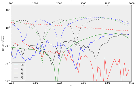
Figure 2: Accuracy of the emulator based on the CFHTemu1 simulations. The figure shows the absolute difference between the descriptor interpolated at the fiducial parameter setting, and the descriptor expected from the CFHTcov simulations (these are the absoulte values of differences which oscillate around zero). The descriptors are shown in units of the standard deviation in each bin $i$ (determined from the diagonal elements of the CFHTcov covariance matrix). We show the accuracy results for the power spectrum (red) and the three Minkowski functionals $V_{0}$ (green), $V_{1}$ (blue) and $V_{2}$ (black). For reference, we also show, using dashed lines, the difference between the expected CFHTcov descriptors and the interpolated descriptor at the non–fiducial point $\mathbf{p}=(0.8,-1.0,0.5)$. This non–fiducial point lies beyond the LM $1\sigma$ contour from the simulations shown in Figure 3 right panel, and corresponds to the target accuracy we wish to achieve

III.3 Dimensionality reduction

The main goal of this work is constraining the cosmological parameter triplet $(\Omega_{m},w,\sigma_{8})$ using the CFHTLenS data. Once the $N\sigma$ contours have been obtained, using the procedure and equations (12)–(16) outlined above, one may ask whether the choice of binning affects these contours. Indeed, in our previous work, we have found that the number of bins, $N_{b}$, can have a non-negligible effect on the contour sizes (see (Petri et al., 2013) for an example with simulated datasets).

In order to ensure that are results are robust with respect to binning choices, we have implemented a Principal Component Analysis (PCA) approach. Our physical motivation for this approach is that, even though we need to specify $N_{b}$ numbers in order to fully characterize a binned descriptor, we suspect that the majority of the constraining information (of a particular descriptor) is contained in a limited number of linear combinations of its binning. In the framework adopted by (Heitmann et al., 2009), for example, the authors find that the majority of the cosmological information in the matter power spectrum is contained in only 5 different linear combinations of the multipoles. Because of this, we believe that dimensionality reduction techniques such as PCA can help deliver accurate cosmological constraints using only a limited number of descriptor degrees of freedom.

In order to compute the principal components of our descriptor space, we use the CFHTemu1 simulations, which sample the cosmological parameters at the $N=91$ points listed in Table 1, and allow us to compute the $N\times N_{b}$ model matrix $M_{pi}=M_{i}(\mathbf{p})$. Note that this is a rectangular (non-square) matrix. Following a standard procedure (see, e.g., ref. (Ivezić et al., 2014)), we derive the whitened model matrix $\tilde{M}_{pi}$, defined by subtracting the mean (over the $N=91$ models) of each bin, and normalizing it by its variance (always over the $N=91$ models). Next we proceed with a singular value decomposition (SVD) of $\mathbf{\tilde{M}}$,

$$\mathbf{U}\mathbf{S}\mathbf{V}^{T}=\frac{\mathbf{\tilde{M}}}{\sqrt{N-1}},$$ (18)

where $S_{ij}=S_{i}\delta_{ij}$ is a diagonal matrix and $V^{T}_{ij}$ is the $j$–th coordinate ($j=1...N_{b}$) of the $i$–th principal component ($i=1...\mathrm{min}[N_{b},N]$) of $\mathbf{\tilde{M}}$, with the index $j$ ranging from $1$ to $N_{b}$. By construction, $\mathbf{V}$ is $\mathbf{p}$–independent.

To rank the Principal Components $V^{T}$ in order of importance, we note that the diagonal matrix $\mathbf{S}^{2}$ is simply the diagonalization of the model covariance (not to be confused with the descriptor covariance in eq. (15)),

$$\frac{1}{N-1}\mathbf{\tilde{M}}^{T}\mathbf{\tilde{M}}=\mathbf{V}\mathbf{S}^{2}\mathbf{V}^{T}.$$ (19)

We follow the standard interpretation of PCA components, stating that the only meaningful components $V^{T}_{i}$ in the analysis (i.e. the ones that contain the relevant cosmological information) are those corresponding to the largest eigenvalues $S^{2}_{i}$, with the smallest eigenvalues corresponding to noise in the model, due to numerical inaccuracies in the simulation pipeline. We expect our constraints to be stable with respect to the number of components, once a sufficient number of components have been included. Using the fact that different principal components are orthogonal, we perform a PCA projection on our descriptor space by whitening the descriptors and computing the dot product with the principal components, keeping only the first $n$ components

$$M(n)_{pi}^{r}=V^{T}(n)_{ij}\tilde{M}_{pj}^{r}\,\,\,\,;\,\,\,\,D(n)_{i}=V^{T}(n)_{ij}\tilde{D}_{j}.$$ (20)

Here we indicate with $V^{T}(n)$ the truncation of $V^{T}$ to the first $n$ rows (i.e. $i$ can now range from $1$ to $n$). As described above, the expectation is that most of the cosmological information is contained in a small number of components $n<N_{b}$. We will describe in detail below the choice we make for $n$, together with the sensitivity of our results to this choice.

Looking at PCA from a geometrical perspective, the dimensionality reduction problem is equivalent to the accurate reconstruction of the coordinate chart of the descriptor manifold. As outlined in ref. (Ivezić et al., 2014), the coordinate chart constructed with the PCA projection in eq. (20) is accurate for reasonably flat descriptor manifolds. When curvature becomes important, more advanced projection techniques (such as Locally Linear Embedding) have to be employed. We postpone an investigation of such improvements to future work.

IV Results

This section describes our main results, and is organized as follows. We begin by showing the cosmological constraints from the CFHTLenS data for the triplet $(\Omega_{m},\sigma_{8},w)$, as well as for an alternative parameterization, $(\Omega_{m},\Sigma_{8},w)$, with $\Sigma_{8}(\alpha)\equiv\sigma_{8}(\Omega_{m}/0.27)^{\alpha}$. In the next section we give a justification on why we fix $\alpha$ to a value of $0.55$. We then use our simulations to perform a robustness analysis of the parameter confidence intervals with respect to the number of PCA components used in the projection. We finally study whether the constraints can be tightened by combining different descriptors. A summary with the complete set of results, along with the relevant Figures, is shown in Table 3.

IV.1 Cosmological constraints

We first make use of equations (12)-(16) to compute the $1\sigma$ constraints on cosmological parameters, using the triplet $(\Omega_{m},\sigma_{8},w)$. Figures 3 shows the constraints in the $(\Omega_{m},\sigma_{8})$ plane, marginalized over $w$, for both the CFHTLenS data, as well as from the mock data in our simulations. In Figure 4, we examine constraints from different sets of moments, as well as using different smoothing scales. Figure 5 shows the confidence contours in the $(w,\Sigma_{8})$ plane, marginalized over $\Omega_{m}$. As this figure shows, and as discussed further below, no meaningful constraints were found on $w$ from CFHTLenS alone.

Because of the relatively small size of this survey, degeneracies among the parameters can have undesirable effects on the constraints. The well-known strong degeneracy between $\Omega_{m}$ and $\sigma_{8}$ is evident in the long “banana” shaped contours in Figures 3 and 4. To mitigate the effect of this degeneracy, in addition to the usual triplet $(\Omega_{m},\sigma_{8},w)$, we consider an alternative parameterization, built with the triplet $(\alpha,\Sigma_{8},w)$ where $\alpha$ is a constant, and $\Sigma_{8}(\alpha)\equiv\sigma_{8}(\Omega_{m}/0.27)^{\alpha}$. While $\Omega_{m}$ and $\sigma_{8}$ are poorly constrained due to degeneracies, the $\Sigma_{8}(\alpha)$ combination lies in the direction perpendicular to the error “banana” at the pivot point $\Omega_{m}=0.27$. This is the direction of the lowest variance $\mathcal{L}(\Omega_{m},\sigma_{8})$ for a suitable choice of $\alpha$, and hence has a much smaller relative uncertainty. We can derive the optimal value of $\alpha$ from the full three dimensional likelihood $\mathcal{L}(\Omega_{m},w,\sigma_{8})$, from which we can compute the expectation values

$$\mathds{E}(\alpha)=\langle\Sigma_{8}(\alpha)\rangle\,\,\,;\,\,\,\mathds{V}(\alpha)=\langle(\Sigma_{8}(\alpha)-\mathds{E}(\alpha))^{2}\rangle$$ (21)

and minimizing the ratio $\sqrt{\mathds{V}}/\mathds{E}$ with respect to $\alpha$. The expectation values are taken over the entire parameter box. This procedure yields a value $\alpha\approx 0.55$ for the statistical descriptors that we consider, consistent with what is found in the literature (see (Kilbinger et al., 2013) for example). Although $\alpha$ can mildly depend on the type of descriptor considered, we choose to keep it fixed, knowing that the width of the $\Sigma_{8}$ likelihood cannot vary significantly with different choices of $\alpha$. We show the probability distribution of the best-constrained parameter $\Sigma_{8}$ (marginalized over $\Omega_{m}$ and $w$) in Figure 6.

We discuss the results of this section in § V below.

IV.2 Robustness

The cosmological constraints should in principle be insensitive to $N_{b}$, once a sufficient number of bins are used, but inaccuracies in the covariance (due to a limited number of realizations) can introduce an $N_{b}$ dependence. Our binning choices are summarized in Table 2. Here we show that the cosmological constraints derived in this paper are numerically robust, i.e. they are reasonably stable, once we consider a large enough number $n$ of Principal Components.

Figure 7 shows the PCA eigenvalues from the SVD decomposition of our binned descriptor spaces (following the discussion in § III.3), as well as the cumulative sum of these eigenvalues, normalized to unity. Figure 8 shows the dependence of the $(\Omega_{m},\sigma_{8})$ constraints on the number of principal components $n$.

These figures clearly indicate that we only need a limited number of components in order to capture the cosmological information contained in our descriptors. The eigenvalues diminish rapidly with $n$, and, in particular, the confidence contours converge to good ($\lesssim 10\%$) accuracy typically for $n=5-10$ (depending on the descriptor). This finding also addresses the inaccuracy of the MF emulator at high thresholds, pointed out in Figure 2. By keeping a limited number of principal components, we are able to prevent the inaccurate high–threshold bins, which have a low constraining power, from contributing to the parameter confidence levels.

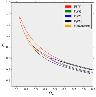
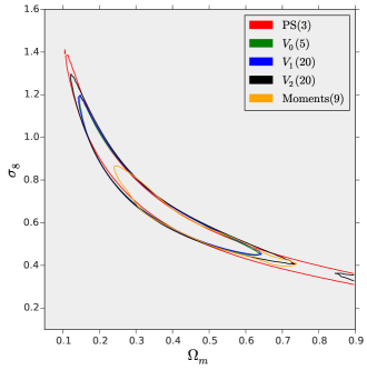
Figure 3: $1\sigma$ (68% CL) constraints on the $(\Omega_{m},\sigma_{8})$ parameter doublet using the power spectrum (red), the three Minkowski functionals ($V_{0}$: green, $V_{1}$: blue, $V_{2}$: black) and the moments (orange). We show the constraints from the data (left panel) and from a mock observation constructed using the mean of 1000 realizations in the CFHTcov simulation suite (right panel). The contours are calculated from the parameter likelihood function $\mathcal{L}$ marginalized over $w$. The parentheses near the descriptor label refer to the number of principal components included.

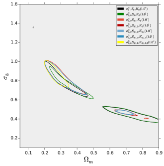
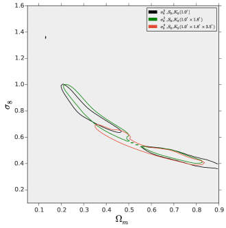
Figure 4: $1\sigma$ (68% CL) constraints on the $(\Omega_{m},\sigma_{8})$ parameter doublet using moments, with different colors corresponding to different moment combinations (see eq. 9 for their definitions). We show the results from the one–point moments $\sigma_{0}^{2},S_{0},K_{0}$ (black curves; both left and right panels). In the left panel, we also show constraints obtained adding moments of gradients to the one–point moments. In the right panel, we combine one–point moments measured at different smoothing scales.

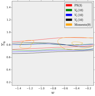
Figure 5: $1\sigma$ (68% C.L.) constraints on the $(w,\Sigma_{8})$ parameter doublet from the CFHTLenS data, obtained with the power spectrum (red), the three Minkowski functionals ($V_{0}$: green, $V_{1}$: blue, $V_{2}$: black) and the moments (orange). The contours are calculated from the parameter likelihood function $\mathcal{L}$ marginalized over $\Omega_{m}$, and the parentheses near the descriptor label refer to the number of principal components.

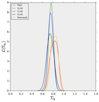
Figure 6: The likelihood of the best-constrained parameter combination $\Sigma_{8}(\alpha)\equiv\sigma_{8}(\Omega_{m}/0.27)^{\alpha}$ from the CFHTLenS data, obtained with the power spectrum (red), the three Minkowski functionals ($V_{0}$: green, $V_{1}$: blue, $V_{2}$: black) and the moments (orange). The likelihood was computed with a constant optimized $\alpha=0.55$, but marginalized over both $\Omega_{m}$ and $w$. The parentheses near the descriptor label refer to the number of principal components.

Parameters	Descriptors	Short description	Relevant Figures
$(\Omega_{m},\sigma_{8})$	PS(3),$V_{0}(5),V_{1}(20),V_{2}(20)$,LM(9)	20cm$1\sigma$ constraints from CFHTLenS
and mock observations	3,3b
$(\Omega_{m},\sigma_{8})$	$(\sigma_{i}^{2},S_{i},K_{i})$	20cm$1\sigma$ constraints from CFHTLenS
using $\kappa$ moments
combined at different $\theta_{G}$	4,4b
$(w,\Sigma_{8})$	PS(3),$V_{0}(10),V_{1}(10),V_{2}(10)$,LM(9)	contours from CFHTLenS	5
$\Sigma_{8}$	PS(3),$V_{0}(10),V_{1}(10),V_{2}(10)$,LM(9)	$\mathcal{L}(\Sigma_{8})$ from CFHTLenS	6
-	PS,$V_{0},V_{1},V_{2}$,LM	PCA eigenvalues	7
$(\Omega_{m},\sigma_{8})$	PS,$V_{0},V_{1},V_{2}$,LM	Stability of contours	8
$(\Omega_{m},\sigma_{8})$	PS(3)$\times V_{0}(5)\times V_{1}(20)\times V_{2}(20)\times$LM(9)	20cmconstraints from CFHTLenS
combining statistics	9
$(w,\Sigma_{8})$	PS(3)$\times V_{0}(10)\times V_{1}(10)\times V_{2}(10)\times$LM(9)	20cmconstraints from CFHTLenS
combining statistics	9b
$\Sigma_{8}$	PS(3)$\times V_{0}(10)\times V_{1}(10)\times V_{2}(10)\times$LM(9)	20cm$\mathcal{L}(\Sigma_{8})$ from CFHTLenS
combining statistics	10

Table 3: Summary of our results and related figures.

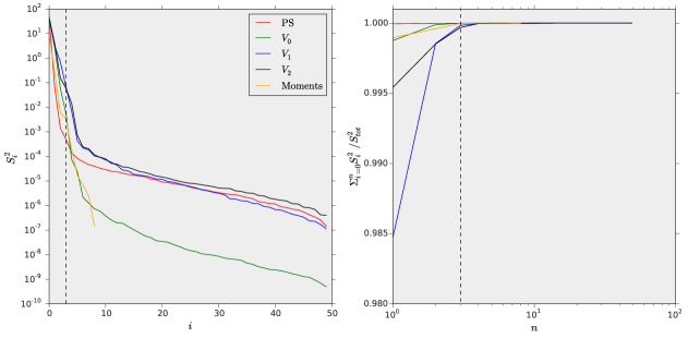
Figure 7: Results from the Principal Components Analysis (PCA) of the binned power spectrum (red), the three Minkowski functionals ($V_{0}$: green, $V_{1}$: blue, $V_{2}$: black) and the moments (orange). The left panel shows the magnitudes of the PCA eigenvalues $S_{i}^{2}$ and the right panel shows their cumulative sum, normalized to unity. A dashed vertical (black) line has marks $n=3$ for reference.

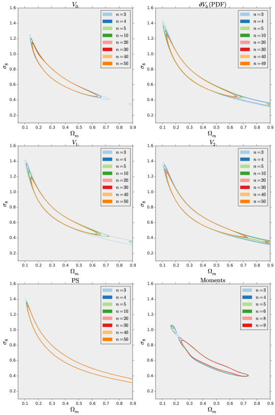
Figure 8: The dependence of the $1\sigma$ contours in the $(\Omega_{m},\sigma_{8})$ plane on the number of PCA components, obtained from a mock observation constructed with the CFHTcov simulations. The different panels refer to the different descriptors (from left to right, top to bottom) $V_{0}$, $\partial V_{0}$(PDF), $V_{1}$, $V_{2}$, power spectrum and moments. The labels in each panel show the number of PCA components included to obtain contour with different colors.

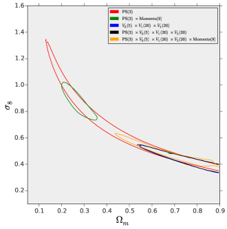
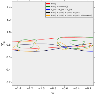
Figure 9: $1\sigma$ constraints on the $(\Omega_{m},\sigma_{8})$ (left panel) and $(w,\Sigma_{8})$ (right panel) doublets, using the power spectrum (PS) alone (red), the MFs alone (blue), as well as using different combinations of descriptors: PS$\times$Moments (green), PS$\times$MFs (black) and PS$\times$MFs$\times$Moments (orange). The likelihood function has been marginalized over $w$ (left panel) and $\Omega_{m}$ (right panel). The parentheses next to each descriptor label refers to the number of PCA components included.

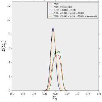
Figure 10: The probability distribution of the best-constrained parameter $\Sigma_{8}$ from the CFHTLenS data, using the power spectrum (PS) alone (red), the MFs alone (blue), as well as using different combinations of descriptors: PS$\times$Moments (green), PS$\times$MFs (black) and PS$\times$MFs$\times$Moments (orange). The likelihood function has been marginalized over $\Omega_{m}$ and $w$. The parentheses next to each descriptor label refers to the number of PCA components.

Descriptor	$\Sigma_{8}=\sigma_{8}\Omega_{m}^{0.55}$
PS(3)	$0.84^{+0.06}_{-0.09}$
PS(3) $\times$ Moments(9)	$0.86^{+0.02}_{-0.09}$
$V_{0}(10)\times V_{1}(10)\times V_{2}(10)$	$0.75^{+0.07}_{-0.04}$
PS(3) $\times V_{0}(10)\times V_{1}(10)\times V_{2}(10)$	$0.76^{+0.04}_{-0.05}$
PS(3) $\times V_{0}(10)\times V_{1}(10)\times V_{2}(10)\times$ Moments(9)	$0.76^{+0.06}_{-0.04}$

Table 4: Tabulated values of $1\sigma$ constraints on $\Sigma_{8}$ corresponding to Figure 10

IV.3 Combining statistics

Different statistics can include complementary cosmological information, allowing their combinations to tighten the constraints. Previous work using multiple lensing descriptors in CFHTLenS alone included combining the power spectrum and peak counts (Liu et al., 2014a), combining the power spectrum and Minkowski functionals  (Shirasaki and Yoshida, 2014) ,and combining quadratic (2PCF) statistics with cubic statistics derived from the 3PCF of the CFHTLenS $\kappa$ field (Fu et al., 2014).

The procedure we adopt here is as follows. Consider two binned descriptors, $d_{1,i},d_{2,j}$ where the indices $i,j$ correspond to bin numbers. We first compute each single–descriptor constraint as a function of the number of PCA components, as in Figure 8. We then determine the minimum number of PCA components $n_{1,2}$ needed for the constraints to be stable. We next construct the vector $d_{1\times 2}=\{d_{1}(n_{1}),d_{2}(n_{2})\}$ and consider this as the combined ($n_{1}+n_{2}$)–dimensional descriptor vector. This procedure naturally allows us to account for the cross–covariance between different binned descriptors. An analogous procedure can be used to combine multiple (three or more) descriptors.

We show constraints from different descriptor combinations in the $(\Omega_{m},\sigma_{8})$ and $(w,\Sigma_{8})$ planes in Figure 9, and on the best-constrained parameter $\Sigma_{8}$ in Figure 10. We also provide a tabulated version of the $\Sigma_{8}$ constraints ($1\sigma$) in Table 4. We discuss these findings in the next section.

V Discussion

In this section we discuss the results shown in § IV above, with particular focus on the constraints on cosmology.

As pointed out in § III.3, the choice of the number of bins, $N_{b}$, is an important issue. In order to ensure that our results are insensitive to $N_{b}$, we adopted a PCA projection technique to reduce the dimensionality of our descriptor spaces. The left panel of Figure 7 shows that the PCA eigenvalues for all of our descriptors decrease by about 4 orders of magnitude from $n=1$ to $n=3$. The right panel of this figure shows that more than 99% of the descriptor variances are captured by including only the first $n=3$ components.

This does not necessarily mean, however, that the cosmological information is captured by the first 3 PCA components: in principle, one of the higher-$n$ PCA components could have an unusually strong cosmology-dependence, and could impact the confidence levels. To address this possibility, we determined the $1\sigma$ contour sizes as a function of $n$ in Figure 8. This figure shows that the first 3 components indeed capture essentially all the information contained in the power spectrum. However, this is not true for the other descriptors. In particular, we find that $n\geq 5$ components are necessary for $V_{0}$, and $n\geq 20$ components for $V_{1}$ and $V_{2}$, in order for the $(\Omega_{m},\sigma_{8})$ contours to be stable at the $\sim$5% level. All nine moments need to be included for the moments contours to be stable to this accuracy.

These results are slightly different when we study the $(w,\Sigma_{8})$ constraints (with $\alpha$ fixed at $\alpha=0.55$ as discussed above). In this case we find that the optimal choice for all three MFs is $n=10$, while the number of components required for the PS and Moments remain at $n=3$ and $n=9$, respectively. (These results are not shown, but obtained analogously to the Figures above.)

We now discuss the main scientific findings of this work. In Figure 3, we show the $1\sigma$ constraints on the $(\Omega_{m},\sigma_{8})$ doublet from the CFHTLenS data. The MF constraints appear to be biased towards the low–$\sigma_{8}$, high–$\Omega_{m}$ region. Here and throughout the remainder of this paper, by ”biased” (or ”unbiased”) we refer to being incompatible (or compatible) with the concordance fiducial values at $1\sigma$ obtained in other experiments. For example, the current best-fit values of $(\Omega_{m},\sigma_{8})=(0.32,0.83),(0.28,0.82)$ from cosmic microwave background anisotropies measured respectively by the Planck  (Planck Collaboration et al., 2014) and WMAP (Hinshaw et al., 2013) satellites lie beyond the 99% likelihood contours obtained from the three MFs (not shown).

This discrepancy may be due to uncorrected systematics in the CFHTLenS data, amplified by the $(\Omega_{m},\sigma_{8})$ degeneracy. As a test of our analysis pipeline, when we try to constrain mock observations based on simulations (shown in the right panel of Figure 3), we recover the correct input position of the $1\sigma$ contours. It is important to note, however, that the mock observations to which the right panel of Figure 3 refers, were built with the mean of $R=1000$ realizations of the CFHTcov simulations. We found that it is possible to find some rare (10 out of the 1,000) realizations for which the best fit for $(\Omega_{m},\sigma_{8})$ lies in the lower right corner, near the location of the best-fit from the data. While this could provide an alternative explanation of the bias from the MFs, the likelihood of this happening is very small ($\lesssim 1\%$).

We observe that the moments give the tightest constraint on $(\Omega_{m},\sigma_{8})$. Furthermore, this constraint is unbiased, in the sense defined above: it includes the current concordance values for these parameters within 1$\sigma$. This leads us to conclude that the bias in the constraints from the MFs is due to systematic errors, rather than the rare statistical fluctuations found above. The fact that the moments are useful for deriving unbiased cosmological constraints has been noted in previous work, which examined the biases caused by spurious shear errors (Petri et al., 2014).

In order to determine the origin of the tight bounds derived from moments, we studied the contribution of each individual moment to the constraints. Figure 4 shows the evolution of the $(\Omega_{m},\sigma_{8})$ constraints as we add increasingly higher-order moments to the descriptor set. Since we are constraining 3 cosmological parameters, we start by considering the set of the three traditional one–point moments which do not involve gradients, i.e. the variance, skewness, and kurtosis $(\sigma_{0}^{2},S_{0},K_{0})$. We then add the remaining six moments of derivatives one by one, starting from the quadratic moments.

Figure 4 shows that the biggest improvement on the parameter bounds comes from including quartic moments of derivatives (i.e. $K_{i}$ with $i\geq 1$) in the descriptor set. This might explain why (Fu et al., 2014) find only relatively weak contour tightening ($\sim 10\%$) when adding three–point correlations to quadratic statistics, since the main improvement comes from higher moments of $\kappa$ derivatives. Ref. (Fu et al., 2014) consider one–point, third–order moments, combined for multiple smoothing scales. Figure 4 explicitly shows, however, that smoothing scale combinations are not as effective as moments of derivatives in constraining the $(\Omega_{m},\sigma_{8})$ doublet. Our results agree with an early prediction (Takada and Jain, 2002) that the kurtosis of the shear field can help in breaking degeneracies between $\Omega_{m}$ and $\sigma_{8}$. Here we found that considering quartic moments of gradients further helps in breaking this degeneracy.

As noted above, the bias in the $(\Omega_{m},\sigma_{8})$ constraints is amplified by the cosmological degeneracy of these parameters. To mitigate this effect, we consider the combination of $\Omega_{m}$ and $\sigma_{8}$ that lies orthogonal to the most degenerate direction, namely $\Sigma_{8}=\sigma_{8}(\Omega_{m}/0.27)^{0.55}$. Figure 5 shows the $1\sigma$ constraints for the $(w,\Sigma_{8})$ doublet, while Figure 6 shows the marginalized $\Sigma_{8}$ likelihood from the CFHTLenS data. The CFHTLenS survey constrains the $\Sigma_{8}$ combination to a value of $\Sigma_{8}=0.75\pm 0.04(1\sigma)$ using the full descriptor set, in agreement with values previously published by the CFHTLenS collaboration (Kilbinger et al., 2013).

These figures also show that the current dataset is insufficient to constrain $w$ to a reasonable precision. This is consistent with the previous analyses of CFHTLenS (Kilbinger et al., 2013; Fu et al., 2014; Liu et al., 2014a; Shirasaki and Yoshida, 2014). We also note that ref. (Shirasaki and Yoshida, 2014) obtained the best-fit value of $w\approx-2$ (but with large errors that include $w=-1$ at 1$\sigma$). We found a similar result when using a Fisher matrix to compute confidence levels. Since the Fisher matrix formalism is equivalent to a linear approximation of our emulator (in which all cosmological parameter dependencies are assumed to be linear), we thus attribute this bias to the oversimplifying assumption of linear cosmology-parameter dependence of the descriptors. Although the right panel in Figure 9 shows that the moments confine $w$ to isolated regions in parameter space, we note that $w=-1$, the value favored by other existing experiments, is excluded at the $1\sigma$ level. The $2\sigma$ contours (not shown in the figure) join, and include $w=-1$.

Regarding the parameter biases, our results overall are in accordance with (Petri et al., 2014), namely, that unaccounted systematics result in larger parameter biases when the constraints are derived from the MFs, and that the LM statistic is less biased. However, for the CFHTLenS data the MFs can still effectively constrain the non-degenerate direction in parameter space, $\Sigma_{8}$ (Figure 6).

Finally, we studied whether the combination of different statistical descriptors can help in tightening the cosmological constraints. We show the effects of some of these combinations in Figures 9 and 10. The left panel of Figure 9 shows that, although combining the power spectrum and the moments with the Minkowski functionals helps tighten the $(\Omega_{m},\sigma_{8})$ constraints, it does not help in reducing the inherent parameter bias of the MFs. The right panel of Figure 9 shows that even with these statistics combined, $w$ remains essentially unconstrained. (Heymans et al., 2013) found that even weak lensing tomography alone is unable to constrain $w$ sensibly. Figure 10 shows that the $\Sigma_{8}$ combination is already well constrained by any of the descriptors alone, without the need of combining different descriptors. This further clarifies that the non–quadratic descriptors mainly help to break degeneracies, tightening contours along the degenerate direction.

VI Conclusions

In this final section we summarize the main conclusions of this work:

• We find that the power spectrum, combined with the moments of the $\kappa$ field provides the tightest constraint on the $(\Omega_{m},\sigma_{8})$ doublet from the CFHTLenS survey data. The tightness of these constraints comes mainly from the moments. Evidence of the unbiased nature of constraints from the moments has been found in (Petri et al., 2014). We further find that the largest improvement on parameter bounds is achieved when we include the quartic moments of derivatives in the descriptor set. This level of improvement cannot be achieved by combining one-point moments at different smoothing scales.

• Although weak lensing surveys are a promising technique to constrain the DE equation of state parameter $w$, reasonable constraints cannot be obtained with the CFHTLenS survey alone, even when using additional sets of descriptors that go beyond the standard quadratic statistics.

• When studying the cosmological information contained in the CFHTLenS data, special attention must be paid to the effect of residual systematic biases. While these residual systematics are found to be unimportant when constraining cosmology with the power spectrum alone, we find that these systematics need to be corrected to obtain unbiased constraints on the $(\Omega_{m},\sigma_{8})$ doublet using the Minkowski functionals. We are aware that, when trying to explain the discrepancy between weak lensing and CMB constraints using the Minkowski functionals, there might be other effects to be considered, namely non–Gaussian error correlations in the descriptors and inaccuracies of the simulations on small scales. These inaccuracies could in principle affect the excursion set reconstruction at high $\kappa_{0}$ thresholds. We will investigate these additional sources of error in future work.

• For the CFHTLenS data set, Minkowski functionals can effectively constrain the non-degenerate direction in parameter space, $\Sigma_{8}$, where the amplifying effects of degeneracy are mitigated.The Minkowski functionals alone are sufficient to constrain the $\Sigma_{8}$ combination to a value of $\Sigma_{8}=0.75\pm 0.04$ at $1\sigma$ significance level. This agrees with the value previously published by the CFHTLenS collaboration within $1\sigma$. Some tensions with Planck (Planck Collaboration et al., 2014) still remain.

Possible future extensions of this work include simulating higher–dimensional parameter spaces (including, for example, the Hubble constant $H_{0}$, and allowing a tilt in the power spectrum or a time-dependence of the DE equation of state $w$), and combining the CFHTLenS constraints with different cosmological probes from large-scales structures and the CMB. The latter can help in breaking the $\Omega_{m},\sigma_{8}$ degeneracy, and allow improvements in the the constraints on $w$. The techniques developed here can be applied to larger, soon-forthcoming survey data sets, such as the Dark Energy Survey (DES) (The Dark Energy Survey Collaboration, 2005), Subaru (Tonegawa et al., 2015), WFIRST (Spergel et al., 2013) and LSST (LSST Dark Energy Science Collaboration, 2012).

References

- Kilbinger et al. (2013) M. Kilbinger, L. Fu, C. Heymans, F. Simpson, J. Benjamin, T. Erben, J. Harnois-Déraps, H. Hoekstra, H. Hildebrandt, T. D. Kitching, Y. Mellier, L. Miller, L. Van Waerbeke, K. Benabed, C. Bonnett, J. Coupon, M. J. Hudson, K. Kuijken, B. Rowe, T. Schrabback, E. Semboloni, S. Vafaei, and M. Velander, MNRAS 430, 2200 (2013), arXiv:1212.3338 [astro-ph.CO] .
- Bernardeau et al. (1997) F. Bernardeau, L. van Waerbeke, and Y. Mellier, A&A 322, 1 (1997), astro-ph/9609122 .
- Hui (1999) L. Hui, ApJ 519, L9 (1999), astro-ph/9902275 .
- Van Waerbeke et al. (2001) L. Van Waerbeke, T. Hamana, R. Scoccimarro, S. Colombi, and F. Bernardeau, MNRAS 322, 918 (2001), astro-ph/0009426 .
- Takada and Jain (2002) M. Takada and B. Jain, MNRAS 337, 875 (2002), astro-ph/0205055 .
- Kilbinger and Schneider (2005) M. Kilbinger and P. Schneider, A&A 442, 69 (2005), astro-ph/0505581 .
- Schneider and Lombardi (2003) P. Schneider and M. Lombardi, A&A 397, 809 (2003), astro-ph/0207454 .
- Takada and Jain (2003) M. Takada and B. Jain, MNRAS 344, 857 (2003), astro-ph/0304034 .
- Zaldarriaga and Scoccimarro (2003) M. Zaldarriaga and R. Scoccimarro, ApJ 584, 559 (2003), astro-ph/0208075 .
- Takada and Jain (2004) M. Takada and B. Jain, MNRAS 348, 897 (2004), astro-ph/0310125 .
- Dodelson and Zhang (2005) S. Dodelson and P. Zhang, Phys. Rev. D 72, 083001 (2005), astro-ph/0501063 .
- Sefusatti et al. (2006) E. Sefusatti, M. Crocce, S. Pueblas, and R. Scoccimarro, Phys. Rev. D 74, 023522 (2006), astro-ph/0604505 .
- Bergé et al. (2010) J. Bergé, A. Amara, and A. Réfrégier, ApJ 712, 992 (2010), arXiv:0909.0529 .
- Jain and Van Waerbeke (2000) B. Jain and L. Van Waerbeke, ApJ 530, L1 (2000), astro-ph/9910459 .
- Marian et al. (2009) L. Marian, R. E. Smith, and G. M. Bernstein, ApJ 698, L33 (2009), arXiv:0811.1991 .
- Maturi et al. (2010) M. Maturi, C. Angrick, F. Pace, and M. Bartelmann, A&A 519, A23 (2010), arXiv:0907.1849 [astro-ph.CO] .
- Yang et al. (2011) X. Yang, J. M. Kratochvil, S. Wang, E. A. Lim, Z. Haiman, and M. May, Phys. Rev. D 84, 043529 (2011), arXiv:1109.6333 [astro-ph.CO] .
- Marian et al. (2013) L. Marian, R. E. Smith, S. Hilbert, and P. Schneider, MNRAS 432, 1338 (2013), arXiv:1301.5001 [astro-ph.CO] .
- Bard et al. (2013) D. Bard, J. M. Kratochvil, C. Chang, M. May, S. M. Kahn, Y. AlSayyad, Z. Ahmad, J. Bankert, A. Connolly, R. R. Gibson, K. Gilmore, E. Grace, Z. Haiman, M. Hannel, K. M. Huffenberger, J. G. Jernigan, L. Jones, S. Krughoff, S. Lorenz, S. Marshall, A. Meert, S. Nagarajan, E. Peng, J. Peterson, A. P. Rasmussen, M. Shmakova, N. Sylvestre, N. Todd, and M. Young, ApJ 774, 49 (2013), arXiv:1301.0830 [astro-ph.CO] .
- Dietrich and Hartlap (2010) J. P. Dietrich and J. Hartlap, MNRAS 402, 1049 (2010), arXiv:0906.3512 [astro-ph.CO] .
- Lin and Kilbinger (2015) C.-A. Lin and M. Kilbinger, A&A 576, A24 (2015), arXiv:1410.6955 .
- Kratochvil et al. (2012) J. M. Kratochvil, E. A. Lim, S. Wang, Z. Haiman, M. May, and K. Huffenberger, Phys. Rev. D 85, 103513 (2012), arXiv:1109.6334 [astro-ph.CO] .
- Petri et al. (2013) A. Petri, Z. Haiman, L. Hui, M. May, and J. M. Kratochvil, Phys. Rev. D 88 (2013), 10.1103/PhysRevD.88.123002, arXiv:astro-ph/1309.4460 [astro-ph.CO] .
- Fu et al. (2014) L. Fu, M. Kilbinger, T. Erben, C. Heymans, H. Hildebrandt, H. Hoekstra, T. D. Kitching, Y. Mellier, L. Miller, E. Semboloni, P. Simon, L. Van Waerbeke, J. Coupon, J. Harnois-Déraps, M. J. Hudson, K. Kuijken, B. Rowe, T. Schrabback, S. Vafaei, and M. Velander, MNRAS 441, 2725 (2014), arXiv:1404.5469 .
- Simon et al. (2015) P. Simon, E. Semboloni, L. van Waerbeke, H. Hoekstra, T. Erben, L. Fu, J. Harnois-Déraps, C. Heymans, H. Hildebrandt, M. Kilbinger, T. D. Kitching, L. Miller, and T. Schrabback, MNRAS 449, 1505 (2015), arXiv:1502.04575 .
- Liu et al. (2014a) J. Liu, A. Petri, Z. Haiman, L. Hui, J. M. Kratochvil, and M. May, ArXiv e-prints (2014a), arXiv:1412.0757 .
- Liu et al. (2014b) X. Liu, C. Pan, R. Li, H. Shan, Q. Wang, L. Fu, Z. Fan, J.-P. Kneib, A. Leauthaud, L. Van Waerbeke, M. Makler, B. Moraes, T. Erben, and A. Charbonnier, ArXiv e-prints (2014b), arXiv:1412.3683 .
- Shirasaki and Yoshida (2014) M. Shirasaki and N. Yoshida, ApJ 786, 43 (2014), arXiv:1312.5032 .
- Erben et al. (2013) T. Erben, H. Hildebrandt, L. Miller, L. van Waerbeke, C. Heymans, H. Hoekstra, T. D. Kitching, Y. Mellier, J. Benjamin, C. Blake, C. Bonnett, O. Cordes, J. Coupon, L. Fu, R. Gavazzi, B. Gillis, E. Grocutt, S. D. J. Gwyn, K. Holhjem, M. J. Hudson, M. Kilbinger, K. Kuijken, M. Milkeraitis, B. T. P. Rowe, T. Schrabback, E. Semboloni, P. Simon, M. Smit, O. Toader, S. Vafaei, E. van Uitert, and M. Velander, MNRAS 433, 2545 (2013), arXiv:1210.8156 [astro-ph.CO] .
- Hildebrandt et al. (2012) H. Hildebrandt, T. Erben, K. Kuijken, L. van Waerbeke, C. Heymans, J. Coupon, J. Benjamin, C. Bonnett, L. Fu, H. Hoekstra, T. D. Kitching, Y. Mellier, L. Miller, M. Velander, M. J. Hudson, B. T. P. Rowe, T. Schrabback, E. Semboloni, and N. Benítez, MNRAS 421, 2355 (2012), arXiv:1111.4434 [astro-ph.CO] .
- Heymans et al. (2012) C. Heymans, L. Van Waerbeke, L. Miller, T. Erben, H. Hildebrandt, H. Hoekstra, T. D. Kitching, Y. Mellier, P. Simon, C. Bonnett, J. Coupon, L. Fu, J. Harnois Déraps, M. J. Hudson, M. Kilbinger, K. Kuijken, B. Rowe, T. Schrabback, E. Semboloni, E. van Uitert, S. Vafaei, and M. Velander, MNRAS 427, 146 (2012), arXiv:1210.0032 [astro-ph.CO] .
- Miller et al. (2013) L. Miller, C. Heymans, T. D. Kitching, L. van Waerbeke, T. Erben, H. Hildebrandt, H. Hoekstra, Y. Mellier, B. T. P. Rowe, J. Coupon, J. P. Dietrich, L. Fu, J. Harnois-Déraps, M. J. Hudson, M. Kilbinger, K. Kuijken, T. Schrabback, E. Semboloni, S. Vafaei, and M. Velander, MNRAS 429, 2858 (2013), arXiv:1210.8201 [astro-ph.CO] .
- Kaiser and Squires (1993) N. Kaiser and G. Squires, ApJ 404, 441 (1993).
- Hinshaw et al. (2013) G. Hinshaw, D. Larson, E. Komatsu, D. N. Spergel, C. L. Bennett, J. Dunkley, M. R. Nolta, M. Halpern, R. S. Hill, N. Odegard, L. Page, K. M. Smith, J. L. Weiland, B. Gold, N. Jarosik, A. Kogut, M. Limon, S. S. Meyer, G. S. Tucker, E. Wollack, and E. L. Wright, ApJS 208, 19 (2013), arXiv:1212.5226 [astro-ph.CO] .
- Heitmann et al. (2009) K. Heitmann, D. Higdon, M. White, S. Habib, B. J. Williams, E. Lawrence, and C. Wagner, ApJ 705, 156 (2009), arXiv:0902.0429 [astro-ph.CO] .
- Springel (2005) V. Springel, MNRAS 364, 1105 (2005), astro-ph/0505010 .
- Lewis et al. (2000) A. Lewis, A. Challinor, and A. Lasenby, ApJ 538, 473 (2000), astro-ph/9911177 .
- Jain et al. (2000) B. Jain, U. Seljak, and S. White, ApJ 530, 547 (2000), astro-ph/9901191 .
- Hilbert et al. (2009) S. Hilbert, J. Hartlap, S. D. M. White, and P. Schneider, A&A 499, 31 (2009), arXiv:0809.5035 .
- Kratochvil et al. (2010) J. M. Kratochvil, Z. Haiman, and M. May, Phys. Rev. D 81, 043519 (2010).
- Munshi et al. (2012) D. Munshi, L. van Waerbeke, J. Smidt, and P. Coles, MNRAS 419, 536 (2012), arXiv:1103.1876 [astro-ph.CO] .
- Matsubara (2010) T. Matsubara, Phys. Rev. D 81, 083505 (2010), arXiv:1001.2321 [astro-ph.CO] .
- VanderPlas et al. (2012) J. T. VanderPlas, A. J. Connolly, B. Jain, and M. Jarvis, ApJ 744, 180 (2012), arXiv:1109.5175 [astro-ph.CO] .
- Note (1) In principle, this assumption could be relaxed, by measuring joint probability distributions of the descriptors in our simulations. In practice, characterizing non-Gaussianities and folding them into the likelihood analysis requires significant analysis, which we postpone to future work.
- Jones et al. (01 ) E. Jones, T. Oliphant, P. Peterson, et al., “SciPy: Open source scientific tools for Python,” (2001–).
- Note (2) Following ref. (Heitmann et al., 2009), we have experimented with interpolations using a Gaussian Process, but did not find a significant improvement in relative error over the much simpler polynomial scheme; this is in agreement with earlier results (see for example (Schneider et al., 2011)).
- Ivezić et al. (2014) Ž. Ivezić, A. Connolly, J. Vanderplas, and A. Gray, Statistics, Data Mining and Machine Learning in Astronomy (Princeton University Press, 2014).
- Planck Collaboration et al. (2014) Planck Collaboration, P. A. R. Ade, N. Aghanim, C. Armitage-Caplan, M. Arnaud, M. Ashdown, F. Atrio-Barandela, J. Aumont, C. Baccigalupi, A. J. Banday, and et al., A&A 571, A16 (2014), arXiv:1303.5076 [astro-ph.CO] .
- Petri et al. (2014) A. Petri, M. May, Z. Haiman, and J. M. Kratochvil, ArXiv e-prints (2014), arXiv:1409.5130 .
- Heymans et al. (2013) C. Heymans, E. Grocutt, A. Heavens, M. Kilbinger, T. D. Kitching, F. Simpson, J. Benjamin, T. Erben, H. Hildebrandt, H. Hoekstra, Y. Mellier, L. Miller, L. Van Waerbeke, M. L. Brown, J. Coupon, L. Fu, J. Harnois-Déraps, M. J. Hudson, K. Kuijken, B. Rowe, T. Schrabback, E. Semboloni, S. Vafaei, and M. Velander, MNRAS 432, 2433 (2013), arXiv:1303.1808 [astro-ph.CO] .
- The Dark Energy Survey Collaboration (2005) The Dark Energy Survey Collaboration, ArXiv Astrophysics e-prints (2005), astro-ph/0510346 .
- Tonegawa et al. (2015) M. Tonegawa, T. Totani, H. Okada, M. Akiyama, G. Dalton, K. Glazebrook, F. Iwamuro, T. Maihara, K. Ohta, I. Shimizu, N. Takato, N. Tamura, K. Yabe, A. J. Bunker, J. Coupon, P. G. Ferreira, C. S. Frenk, T. Goto, C. Hikage, T. Ishikawa, T. Matsubara, S. More, T. Okumura, W. J. Percival, L. R. Spitler, and I. Szapudi, ArXiv e-prints (2015), arXiv:1502.07900 .
- Spergel et al. (2013) D. Spergel, N. Gehrels, J. Breckinridge, M. Donahue, A. Dressler, B. S. Gaudi, T. Greene, O. Guyon, C. Hirata, J. Kalirai, N. J. Kasdin, W. Moos, S. Perlmutter, M. Postman, B. Rauscher, J. Rhodes, Y. Wang, D. Weinberg, J. Centrella, W. Traub, C. Baltay, J. Colbert, D. Bennett, A. Kiessling, B. Macintosh, J. Merten, M. Mortonson, M. Penny, E. Rozo, D. Savransky, K. Stapelfeldt, Y. Zu, C. Baker, E. Cheng, D. Content, J. Dooley, M. Foote, R. Goullioud, K. Grady, C. Jackson, J. Kruk, M. Levine, M. Melton, C. Peddie, J. Ruffa, and S. Shaklan, ArXiv e-prints (2013), arXiv:1305.5422 [astro-ph.IM] .
- LSST Dark Energy Science Collaboration (2012) LSST Dark Energy Science Collaboration, ArXiv e-prints (2012), arXiv:1211.0310 [astro-ph.CO] .
- Schneider et al. (2011) M. D. Schneider, Ó. Holm, and L. Knox, ApJ 728, 137 (2011), arXiv:1002.1752 .