OIQP-15-01
Negative anomalous dimensions in SYM
Yusuke Kimura***londonmileend@gmail.com and Ryo Suzuki†††Ryo.Suzuki@maths.ox.ac.uk
∗Okayama Institute for Quantum Physics (OIQP),
Kyoyama 1-9-1, Kita-ku, Okayama, 700-0015, JAPAN
†Mathematical Institute, University of Oxford,
Andrew Wiles Building, Radcliffe Observatory Quarter,
Woodstock Road, Oxford, OX2 6GG, UK
Abstract
We elucidate aspects of the one-loop anomalous dimension of -singlet multi-trace operators in SYM at finite . First, we study how corrections lift the large degeneracy of the spectrum, which we call the operator submixing problem. We observe that all large zero modes acquire anomalous dimensions starting at order with a non-positive coefficient and they mix only among the operators with the same number of traces at leading order. Second, we study the lowest one-loop dimension of operators of length equal to . The dimension of such operators becomes more negative as increases, which will eventually diverge in the double scaling limit. Third, we examine the structure of level-crossing at finite in view of unitarity. Finally we find out a correspondence between the large zero modes and completely symmetric polynomials of Mandelstam variables.
1 Introduction
Large gauge theories have been intensively studied for decades since the work of ’t Hooft, who discovered that mesons are described by a string in the planar limit [1]. Maldacena argued that a -dimensional gauge theory can be described by a -dimensional gravity theory, which is now called the AdS/CFT correspondence [2].
The primary example of the AdS/CFT correspondence is the one between maximally supersymmetric Yang-Mills theory in four dimensions ( SYM) and superstring on AdSS5 in the planar limit. Integrability is a powerful technique in this setup, which makes it possible to compute conformal dimensions of gauge-invariant operators in SYM and the energy of AdSS5 superstring states at any value of the ’t Hooft coupling (see [3] for a review). In contrast, the non-planar problems are notoriously complicated and less well-understood. The entire problem seems daunting, but we shall present a tractable corner of it. The purpose of this paper is to look for simple structures in the non-planar problem and to provide a new point of view on the large problems.
Our motivation is explained in three ways. The first one is to better understand the AdS/CFT correspondence at finite .
The second one is to study operators with negative anomalous dimensions. Since all planar anomalous dimensions are non-negative, negative anomalous dimensions are inevitably a non-planar effect. In addition, corrections to the dimension of double-trace operators are related to four-point functions. The four-point functions on the gravity side are related to the phase shift of a high-energy scattering [4, 5, 6], which must be positive in order to preserve the asymptotic causality of spacetime [7]. Thus, the AdS/CFT and causality predict that certain double-trace operators should have negative anomalous dimensions. We want to observe similar phenomena in SYM, though the operators of concern are different from [7].
The third one is to inspect the large behavior of determinant-like operators with all non-planar corrections taken into consideration. It was found in [8, 9] that, if we take the naïve ’t Hooft limit and apply integrability methods, then the dimensions of the double-determinant operators, which correspond to the energies of a pair of open string tachyons between a D-brane and anti-D-brane, becomes either divergent or complex at two-loops. Since any operators of SYM have perturbatively real and finite anomalous dimensions at finite , such pathological behavior should be remedied with non-planar effects.
Given this situation, it is worthwhile to look for an alternative to integrability to study the non-planar problem. A promising approach is the group theoretical method initiated by [10]. This method is based on the construction of a basis of local operators that diagonalizes the free two-point functions. The work [10] dealt with the 1/2 BPS sector, and later it was extended to more general sectors. The basis of [11, 12] is suitable for describing open string excitations on giant gravitons, and the bases in [13, 14, 15] were designed by Brauer algebras. The flavor symmetry is manifested in the bases of [16, 17]. One common feature of the diagonal bases is that they are labeled by a set of Young diagrams. It was also observed that the one-loop mixing is highly constrained on these bases — two operators can mix if their Young diagrams are related by moving a single box of the Young diagram [18, 19, 20, 21]. This property makes the problem tractable, and in certain situations it is possible to obtain the spectrum of the dilatation operator explicitly [22, 23, 24, 25, 26, 27]. Although we have realized these bases are useful tools for the non-planar mixing problem, most results have been limited to the sector. One motivation of this work is to explore the non-planar mixing problem of the sector.111The sector consists of gauge-invariant local operators made out of two holomorphic scalars, which are closed under the operator mixing to all orders of perturbation theory in SYM. The sector is made out of six real scalars and closed at one-loop.
The non-planar dilatation operator in the one-loop sector was written down in [28, 29],
| (1.1) |
and the general non-planar spectrum has been studied in many ways [30, 31]. In the planar limit, the Bethe Ansatz Equations give us the spectrum of all single-trace operators in the sector [32]. Naturally, one hopes to know the spectrum of all multi-trace operators at arbitrary . This problem has not been studied thoroughly. One of the main difficulties is that the number of operators involved in the mixing grows factorially with respect to the operator length . For example, there are 469 scalar singlet multi-trace operators at , and 4477 operators at . By brute-force computation, we managed to compute explicitly the matrix elements of the non-planar mixing and obtained their eigenvalues up to . Various interesting properties of our results are explained below.
At , the anomalous dimensions are highly degenerate, and this is why the planar mixing problem is integrable. Most of the large degeneracy are lifted by corrections. We focus on the degenerate eigenstate having the zero anomalous dimension at large , which we call the operator submixing problem. The submixing problem at can be solved by diagonalizing the Hamiltonian
| (1.2) |
where is the projector to the space of the large zero modes. We observed remarkable patterns among the solutions up to , and conjecture that these patterns continue for any . In particular, each eigenstate is a sum of multi-trace operators with the same number of traces, and all eigenvalues are non-positive:
| (1.3) |
where is the one-loop anomalous dimension.
Besides the dilatation operator, higher-point correlation functions offer an alternative route to compute the corrections to the operator dimension or string energy. For example, by studying the OPE expansion of the four-point functions of single-trace operators, one can compute the correction to the dimension of intermediate states, which are double-trace operators at large . This problem has been explored in the literature on the AdSS5 side [33, 34, 35, 36, 37], the SYM side [38, 39, 40, 41], and via the conformal bootstrap [42, 43, 44, 45, 46]. Following this line of development, we consider four-point functions of multi-trace operators in Section 4, and argue that they constrain the eigensystem of submixing matrices.
In Section 5 we discuss the following aspects of the finite spectrum:
The one-loop dimension of determinant-like operators generally receives non-planar corrections even in the large limit, because their operator length is of order . The proper way to take the large limit is to study their dimension at a finite and extrapolate the results to . This result can be different from the naïve limit, where we first take the large limit and identify a double-determinant-like operator as a state of an integrable open spin chain with boundaries. We are interested in the operators with length , with the hope that non-planar corrections rescue the pathological behavior of the double-determinant operator found in [8]. Indeed, we find an operator with whose one-loop dimension is zero at any , which may be regarded as a non-planar completion of the double-determinant operator. In addition, we also find an operator with a lower dimension by studying dilatation eigenstates at up to . The lowest-energy state has a negative one-loop dimension which decreases as increases. This anomalous dimension will eventually diverge in the large limit,222Of course, the tree-level dimension of the double-determinant is , which diverges in the large limit. Here we argue that the anomalous dimension in the sector diverges. This situation is different from the one in the sector, where the determinant operator dual to giant graviton is BPS [47], and the determinant-like operators have finite anomalous dimensions in the large limit and are computed by the energy of an integrable open spin chain [48, 49].
| (1.4) |
We investigate level-crossing: whether the adjacent one-loop dimensions or energy levels cross at finite . According to the non-crossing rule of von Neumann-Wigner [50], there should be no level-crossing if the Hamiltonian of the system has no extra symmetry. We find that most of the energy levels do not cross for but do collide for , which can be explained by the non-Hermiticity of the operator mixing matrix and the finite constraints.
The one-loop dimensions exhibit eccentric behaviors for , which makes it difficult to keep track of the dilatation eigenstates (or SYM operators) from large to small . In other words, when we regard the one-loop dimension as an analytic curve on the plane, we are not able to tell which curve corresponds to which SYM operator unambiguously. To support this idea, we construct an automorphism which relates high energy states and low energy states.
Finally, Section 6 is devoted to Discussion and Outlook.
Appendices are organized as follows. Our notation is explained in Appendix A. The one-loop spectrum at finite is summarized in Appendix B. The details of computations on correlation functions are given in Appendix C. The intriguing relation between the number of singlet large zero modes and the completely symmetric polynomial of Mandelstam variables is discussed in Appendix D. A concise way of describing multi-trace operators is introduced in Appendix E, where we briefly explain our idea behind Mathematica implementation. This paper is accompanied by a Mathematica notebook and a data file which contain the operator mixing matrix at discussed in Appendix B.2.
2 Operator (sub)mixing problem
2.1 Synopsis
We start with a brief review on the operator mixing problem. In SYM at weak coupling, the two-point functions of scalar operators behave as333Note that in logarithmic CFT.
| (2.1) |
where and are and come from finite and singular counterterms, respectively [40]. The quantity is related to the one-loop mixing matrix, or the one-loop dilatation operator. By using the eigenstates of we can rewrite the two-point function into the familiar form
| (2.2) |
Note that is generally not Hermitian even though are Hermitian [51, 29].
The dilatation operator is self-adjoint with respect to the two-point functions, which can be shown by the spacetime translational symmetry as
| (2.3) |
If are the eigenstate of the dilatation operator , we obtain
| (2.4) |
Below we investigate the case and , where the spectral degeneracy among the large zero modes is lifted by corrections. This problem is what we called the operator submixing in Introduction.
We want to diagonalize the submixing matrix. This problem may look simple because the dimension of the submixing matrix, namely the number of the large zero modes, is significantly smaller than the number of all operators. Nevertheless, it contains rich information about non-planar interactions.
The submixing equation itself determines the eigenstates at the zeroth order of expansion. We focus on the problem at , because in SYM, the degeneracy of the large zero modes is mostly lifted at this order. Still, some eigenvalues may remain degenerate.
2.2 Lifting the large degeneracy
Let us derive submixing equations. We are mostly interested in the submixing among the large zero modes, namely the operators with the vanishing anomalous dimension at . The large zero modes in the scalar singlets will be given explicitly in Section 2.3.
Let and be the space of the large zero modes and non-zero modes, respectively. We split the dilatation operator into the planar and non-planar part as , and regularize the planar part by to make it invertible. Take a general linear combination of the large zero modes, and call it . is regarded as the large limit of a finite eigenvector . Then the non-planar operator mixing equation becomes
| (2.5) |
Expand this equation in and apply . The results are
| (2.6) |
We take the limit and keep track of the singular terms. Denote the matrix elements of and by
| (2.7) |
where are the non-zero eigenvalues of . The projector to is written as
| (2.8) |
The projector to is . We also use the notation .
The equation can be written as
| (2.9) |
The limiting behavior of the operator depends on the operand; it is singular on and regular on . By evaluating up to second order and using and , we obtain
| (2.10) | ||||
| (2.11) | ||||
| (2.12) |
By extracting the components of in and , one finds
| (2.13) |
The first equation determines the eigenvalue , which may lift the large degeneracy. The second equation determines but not . No equations can constrain because are the zero modes of the planar dilatation. They cannot be fixed by perturbation at -th order. These zero modes are not important at , because the eigenvalue does not depend on as shown below.
2.2.1 Matrix elements
Let us rewrite the above equations in terms of matrix elements. We use small or capital letters in place of or to label the components of or , respectively. An eigenstate is expanded as . Equations become,444Note that and do not depend on .
| (2.14) |
Collecting the terms leading in the limit at , we obtain,
| (2.15) |
These are the equations for degenerate perturbation at first order. In Appendix B.2, we observe that the large degeneracy of zero modes in SYM is not lifted at first order. Therefore, we assume
| (2.16) |
At , we find
| (2.17) | ||||
| (2.18) |
The first line is the submixing equations because it lifts most of the large degeneracy at . This equation is insensitive to the ambiguity of . The second line determines the eigenstates .
2.3 Large zero modes
We classify the large zero modes in the singlet representation of .
The BPS states of SYM can be labeled by the irreducible representations of [52] (see also [53]). The conformal part of the algebra can be neglected if we focus on primary operators. Let us denote by the single-trace operator consisting of scalars whose flavor indices are traceless and symmetric. General half-BPS multiplets belong to the representation . 555Here denotes Dynkin labels of . The primary operators can be written at large as
| (2.19) |
Similarly, quarter- and eighth-BPS primary operators can be written at large as
It is not easy to write down BPS operators explicitly at finite because one has to solve the mixing problem coming from the color structure [38, 54, 55]. Recent attempts at solving the zero eigenvalue equation of the dilatation operator are available in [56, 57, 58, 23, 25].
One can prove that a large zero mode is always written as a product of ’s. At large , the anomalous dimension of a multi-trace operator is the sum of the anomalous dimension of the constituent single-trace operators. The dimensions of the single-traces are given by the planar dilatation, which is equal to an integrable spin-chain Hamiltonian. The planar dilatation has the ground state given by the traceless symmetric single-trace operator, which is , and its eigenvalues are non-negative. Note that the products of BPS operators are non-BPS in general.
We present examples of scalar multi-trace operators in singlet with the vanishing anomalous dimension at large . For clarity, we introduce the flavor indices
| (2.20) |
where means traceless and completely symmetric. Then, the large zero modes with length are given by
| (2.21) |
The number of the large zero modes with length , denoted by , grows as in Table 1.
| 2 | 4 | 6 | 8 | 10 | 12 | |
|---|---|---|---|---|---|---|
| 0 | 1 | 2 | 5 | 11 | 34 | |
| 1 | 4 | 15 | 71 | 469 | 4477 |
Finding an explicit formula for is a difficult problem of combinatorics. Interestingly, this series coincides with the asymptotic number of completely symmetric polynomials of Mandelstam variables at degree subject to the massless momentum conservation [59, 60], which will be further explained in Appendix D. This coincidence may break down at due to the finite - constraints, where in SYM. An example of the finite - constraints is the following anti-symmetrization identity:
| (2.22) |
which reduces the number of independent large zero modes by one.
2.4 Observations on submixing
We present here interesting structure found in the submixing. The data in Appendix B.2 is summarized in Figure LABEL:fig:lam2, which shows the eigenvalues of the submixing Hamiltonian for . The one-loop anomalous dimension is given by . The legend “-tuple trace" means that the operator consists of a mixture of -trace operators at large . At higher orders, they mix with everything else. Also, the numerical values of for the operators starting from double-traces are shown in Table LABEL:tab:gam2-dt.
Let us rephrase our findings. First, most of the large degeneracy of zero modes is lifted at second order. This statement is not trivial because the large degeneracy of non-zero modes is sometimes lifted at the first order in .
Second, all the second-order eigenvalues are non-positive, . This is again non-trivial despite the minus sing in , because the matrix elements are not symmetric, . Note that the finite anomalous dimensions of the large zero modes can be positive. There exist operators with and for some .
Third, when the large degeneracy of zero modes is lifted at , all eigenstates have a definite number of traces. Thus, the submixing Hamiltonian should commute with the operator which counts the number of traces. In contrast, the operators with different number of traces may submix for the large non-zero modes.
Fourth, if we define the density of submixing matrix elements by applying the Laplace transform to as666There can be other integral representations of .
| (2.23) |
the submixing densities at different satisfy
| (2.24) |
where is the projector to , which is the subspace of spanned by the products of length-two operators. This “projective commutation” relation is equivalent to
| (2.25) |
for . These relations imply that the submixing problem on is integrable.
It will be interesting to prove these findings and see how general these relations hold true, which will help to solve general submixing problem. The projection by may be removed by finding a better definition of the submixing density, or equivalently a better definition of mutually commuting charges .
2.5 How to solve non-planar operator mixing
Let us pause to explain how we obtained the aforementioned results on the operator submixing. It is not a priori clear at which order the large spectral degeneracy is lifted, so we need to study the general non-planar operator mixing problem. Since the full non-planar problem is too complicated to work by hand, we used computer programs extensively to obtain concrete results. More specifically, we wrote Mathematica codes and proceed as follows,
-
•
Generate a complete set of multi-trace operators with a given length, using the notation in Appendix E.
-
•
Compute the action of one-loop dilatation operator on the complete set of multi-traces.
-
•
Extract the matrix elements, as analytic functions of and .777 SYM corresponds to . We introduced a parameter as discussed in Appendix A.
Our computation can be done symbolically with no numerical errors until this stage. See the attached Mathematica code for details.
Having obtained explicit non-planar mixing matrices, we will study their eigensystems later in this paper. We will analyze
-
•
Operator submixing problem as perturbation
-
•
Eigenvalues as analytic functions of and
-
•
Finite constraints on eigenvectors
There is no need to invent new techniques to solve these standard problems of linear algebra. In order to manage large matrices (of size ) efficiently, one should compute their eigenvalues numerically at . It will take an extremely long time to find all eigenvalues analytically if the matrix size is bigger than .
It is not easy to inspect carefully the Mathematica codes, so we need to check that no mistakes were made during the computation, which can be done in two ways. First, our mixing matrix eigenvalues at agreed analytically with the literature [61, 62] as shown in Appendix B.2. Second, all eigenvalues of the mixing matrix are real. This is a non-trivial check because we computed the mixing matrix elements using the basis in which the matrix is non-hermitian. Further discussion on the finite spectrum will be given in Section 5.
3 Correlation functions
We will study the submixing problem by evaluating two-point functions. First we evaluate in terms of correlation functions of , and derive the submixing Hamiltonian. Then we discuss the sign and the -dependence of .
3.1 Preliminary
In this subsection, we summarize preliminary facts about correlation functions.
We will focus on color and flavor combinatorial factors of correlation functions, and we drop the space-time dependence, which is trivial to recover from conformal invariance. In our analysis, the difference between the gauge group and the gauge group does not matter because we mainly discuss the leading large contribution. We use the Wick-contraction
| (3.1) |
It can be extended to the case of multi-fields as
| (3.2) | |||||
where the normal ordering defines an operator without self-contractions. Because of the normal ordering, Wick-contractions apply only between and .
Next gauge invariant operators are considered. Any multi-trace gauge invariant operator built from matrices can be characterized by an element of the symmetric group as
| (3.3) | |||||
Focusing only on the color structure by leaving out the flavor indices, this description has the symmetry
| (3.4) |
where is any element in . This implies that the multi-trace structure of gauge invariant operators is classified by the conjugacy classes of , which are the partitions of . It is then straightforward to obtain two-point functions for gauge invariant operators [17],
| (3.5) | |||||
We introduced a shorthand notation
| (3.6) |
and counts the number of cycles in the permutation , e.g. , .
Finding the -dependence of the correlator is a complicated combinatorial problem with the color and flavor structures correlated. In Section 3.3, we will concretely compute the two-point functions of the double-trace large zero mode, as an example to see how the correlators depend on .
In the literature [16, 17, 14], bases of gauge invariant operators in the scalar sector have been constructed, and they diagonalize the two-point functions including all corrections. The readers can also refer to [10, 13, 12, 63], although we do not need those technologies in what follows.
When and are in the same conjugacy class (i.e. they have the same trace structure), the two-point functions behave as . Its coefficient is a symmetry factor determined by the number of permutations satisfying ,888 The symmetry factor of the two-point functions can be associated with group theory. Suppose is in the conjugacy class , where is the number of cycles of length , i.e. . The number of permutations satisfying is counted as follows. For a cycle with length , there are exactly cyclic permutations that do not change the cycle. Hence, cyclic permutations can leave the cycles. Also, can permute cycles of the same length. Then we have the formula (3.7) For in the conjugacy class , we have . For in the conjugacy class , we have .
| (3.8) |
On the other hand, if and are not in the same conjugacy class, (i.e. they have different trace structure), the two-point functions behave as with . In other words, for two normalized operators , we have
| (3.9) |
if they have the same trace structure, and
| (3.10) |
if they have different trace structure.
We can also deduce the large behavior of matrix elements of the dilatation operator. The planar dilatation operator does not change the number of traces while the non-planar dilatation operator does change the number of traces by one. In other words, the planar dilatation operator does not change trace structure of operators while the non-planar operator does. As a consequence we find
| (3.11) |
and so on, where is a linear combination of operators with the same trace structure.
We expand a dilatation eigenstate as
| (3.12) |
where each field is allowed to be a linear combination of multi-traces. We will assume that the two-point function between and is subleading
| (3.13) |
For example, if is a double-trace operator, can be a linear combination of single-traces and triple-traces. This assumption is essential in the subsequent argument, and it is desirable to have a proof.
Note that correlation functions of like have a meaningful expansion only if . In general, the numerical factor appearing in each order of the expansion is a function of or , where is a partition of . Hence the expansion parameter in and is . In order for this expansion to be a perturbative expansion, we need to assume , which we do in what follows. Then, two-point functions of reduce to those of in the planar limit.
3.2 Correlator expressions of
3.2.1 perturbation revisited
The dilatation operator can be divided into the planar and non-planar parts,
| (3.14) |
We will study the case is given by a linear combination of the large zero modes, which is characterized by
| (3.15) |
Substituting the expansions into the eigenvalue equation
| (3.16) |
we have
| (3.17) |
Taking the two-point functions of this equation with leads to
| (3.18) |
From the fact that the dilatation operator is self-adjoint with respect to the two-point function, we have
| (3.19) |
Because , we obtain
| (3.20) |
Assuming that and have different trace structure, we see that the expansion of starts from the order .999This situation is parallel to our argument around . Substituting into , we find
| (3.21) |
where is a linear combination of multi-traces that are different from . Considering the two-point functions of and , we obtain
| (3.22) |
which is consistent with our assumption .
The equation (3.21) can be used to get the following expression,
| (3.23) |
or equivalently by expanding ,
| (3.24) |
This expression of will be frequently used later. Because is the leading term of the expansion, we can use the planar limit to compute the correlation functions.
3.2.2 Submixing Hamiltonian
Let us derive the submixing Hamiltonian. We use a Greek letter to label different large zero modes as
| (3.27) |
For simplicity, we assume that the eigenvalues are non-degenerate, for . By generalizing the above argument, we obtain
| (3.28) | |||||
The left-hand side is proportional to , so the right-hand side is. Since spans the entire Hilbert space of the large zero modes, we can think of as an operator identity,
| (3.29) |
which is .
In Section 3 we will rewrite the submixing equation in the operator form,
| (3.30) | |||
| (3.31) |
We call submixing Hamiltonian. The projector is needed because maps to the whole space of operators, . Note that the first term in vanishes if we write down matrix elements as in Section 2.2 owing to . The (dis)appearance of the first term originates from the fact that the mixing matrix is not Hermitian whereas the dilatation operator is self-adjoint with respect to the two-point functions.
We can also rewrite the submixing density into an operator form as
| (3.32) |
The integral over converges if we consider thanks to and . Then we can safely take the limit .
For the double-trace operator , the action of the submixing Hamiltonian can be schematically represented as
| (3.33) |
where each circle represents the single-trace operator . The , represented by a gray circle, is an interaction vertex and is a propagator. The intermediate state in the second term must be a single-trace.
In the literature, the energy spectrum of string in pp-wave SFT was compared with the dimension of BMN-type operators in SYM. It was argued that we should include four-point contact terms in the pp-wave SFT for a better agreement and to cancel a divergent term from a cubic coupling [64, 65]. We can interpret the first term in as the four-point contact term, and the second term as the cubic term squared, in consistent with the expectation from the pp-wave SFT.
Interestingly, we can remove the four-point contact term if we renormalize the wave-function as . From it follows that , which contains only the propagator .
3.2.3 On the sign of
Here is another comment on the sign of . The eigenvalues of are non-negative, but it does not mean is non-positive. Let be an eigenbasis of , respectively. The state can be expanded as
| (3.34) |
Note that is not an orthogonal transformation, because is not an orthonormal basis at finite . It follows that
| (3.35) |
Since and have different spectra at finite , can be positive or negative.
3.3 Two characteristic classes of the large zero modes
As we mentioned in Section 2.4, the submixing pattern can be classified by the number of traces of the large zero modes. We will focus on the two characteristic cases in the classification: the number of traces being minimal or maximal. The first case is the double-trace operator , which is the unique operator of length with two traces. The second case is a set of operators having the largest number of traces, namely -tuple length-2 operators such as . The number of such operators is equal to the number of partitions of excluding the partitions that contain 1. Let us introduce a shorthand notation . There are two operators for ; and , and there are four operators for ; , , and . For , the constraint (2.22) has to be taken into account.
Below we want to see how the -dependence arises from correlation functions, by taking the double-trace operator as the simplest example. In general, the two-point functions of other large zero modes result in complicated combinatorial problems.
We write the singlet double-trace operator as
| (3.36) | |||||
where represents the conjugacy class of cycle length in . We introduced the projection operator associated with the rank- symmetric traceless representation of .

From the formula (3.5), the two-point functions of can be computed as
| (3.37) |
To simplify it, let us use the diagrammatic computation presented in [66, 13] and Figure 1. We also introduce a trace over , where is a 6-dimensional vector space for the flavor index. It follows that101010With the notation , is the contraction between the -th space in the former and the -th space in the latter .
| (3.38) |
where is the trace over . The factor at the second line originated in the symmetry that exchanges two ’s of the operator. At the third equality, and are permutations satisfying (see footnote 8), and we have used
| (3.39) | |||||
where we used and . The second equality can be explained by Figure 1 without permutation . is the dimension of the totally symmetric traceless representation of .
3.4 Evaluating
We now evaluate based on the expression (3.24).
First, we see that the dilatation operator annihilates the single-trace operator . The first term of the dilatation operator annihilates because the indices are symmetrized, and the second term annihilates because the indices are traceless. Then, the dilatation operator acts on the product as
| (3.40) |
The two derivatives in the dilatation operator do not act on the same single-trace.
With the above facts, we will turn to the correlator expression of . Suppose that the dilatation operator acts locally on the factor
| (3.41) |
contained in . The effect of the non-planar dilatation operator is to make a single-trace from the double-trace, which we find from the formula (A.7)-(A.14), reducing the number of traces of by one. The total action of the dilatation is the sum of local actions on each pair of single-traces.
From the intuition of AdS/CFT, we may regard as a two-string state. A single-string state is also created by the action of the dilatation. In this sense, the first term of in (3.24) is considered to be the overlap between the two-string and single-string states, and the second term of can be interpreted to be the planar energy of the single-string state.
We next discuss the sign of in (3.24). Recall that the numerical study for shows that is always non-positive for given by a linear combination of the large zero modes. It is easy to see that the second term of is non-positive because the eigenvalues of the planar dilatation operator are non-negative. The sign of the first term is non-trivial because the non-planar dilatation operator contains several terms with different signs.
In order to get more insight on , we will analyze the correlation functions exploiting a large limit, which is defined by letting the flavor indices run over and by taking . (In Appendix C we will realize that appears with a factor .) This limit describes the case in a good numerical accuracy for small as will be shown in Figure 13. Thus, we expect that the anomalous dimension as given by the ratio of correlators is not very sensitive to the value of .
Concrete computations are doable at large , as will be given in Appendix C. In Appendix C.1 we will show that the first term of in (3.24), , is non-positive. In Appendix C.2 we will compute for the two classes of the large zero modes presented in the last subsection. We write for the double trace operator and for the -trace operators.
In general, the first term of is of order while the second term is of order . Only the second term, , is important at large . For the double-trace operator (3.36), our result (C.21) reads
| (3.42) |
where is an -independent constant that may depend on . In view of the AdS/CFT correspondence, the double-trace operator would correspond to a non-supersymmetric two-string state, where each string has the angular momentum with the opposite sign. Then measures the energy difference between the two-string state and that of the bound state. As becomes large, one needs the more energy to break the bound state into the oppositely-rotating two-string state. This interpretation is consistent with the numerical results suggesting that is an increasing function of .
For -trace operators, we have the following result (C.29),
| (3.43) |
where specifies an eigenstate among various -trace operators, and is another -independent constant. More details are presented in Appendix C.2. These operators should correspond to bound states of non-supersymmetric -particles rather than strings.
Finding the exact dependence of the submixing eigenvalues is a future problem. One of the main obstacles is to compute the inverse of the planar dilatation operator . The eigenstates of can be readily constructed by using the integrability methods, but one needs to solve combinatorial problems to expand the states and in terms of the planar eigenstates. Group-theoretical methods will be useful for this purpose. The limit with is also worth investigation. Our results imply that the expansion parameter, or the effective string coupling, in this region is for and
4 Submixing from four-point correlators
We discuss the relation between operator submixing problem and four-point functions of multi-trace operators.
Consider the four-point function of half-BPS operators, . The four-point function of SYM can be decomposed into a product of three-point couplings and superconformal blocks [69]. By expanding the four-point function in Taylor series around , we obtain a sum of anomalous dimensions averaged over all possible intermediate operators of given quantum numbers, where the weight of average is given by the product of three-point couplings.
If we normalize the two-point functions as , the perturbative part of the four-point function scales as in the large limit [67, 68]. The three-point coupling scales as if the intermediate operator has the same trace structure as , and otherwise. For the former case, the anomalous dimension of the intermediate operator should scale as . If not, the anomalous dimension scales as . This structure is illustrated in Figure 2.

The case of has been studied in detail in [40]. From the four-point function , we can extract the contribution of singlets which propagate along the internal line. There are four singlets at twist four, corresponding to the states . If we denote the eigenvalues of the one-loop dilatation operator by , we obtain
| (4.1) |
at . The negative sign of originates from the negative-mode of double-trace type, .
General submixing problem beyond the double-trace is related to the four-point functions of products of half-BPS operators. A simple example is
| (4.2) |
whose OPE decomposition contains information about the triple-trace operator . Although product operators like are not dilatation eigenstates at finite , we can neglect corrections by taking the large limit in what follows.
Some multi-trace four-point functions are or less. In such situations, we can deduce constraints on the eigensystem of submixing matrices. Consider the multi-trace four-point function shown in Figure 3,
| (4.3) |
Since has the color structure of the five-point function of half-BPS operators, it scales as at large . Thus we find
| (4.4) |
which implies
| (4.5) |
Is there a situation where both and are ? It can happen if an intermediate operator is given by a linear combination of the double-trace and triple-trace large zero modes,
| (4.6) |
If is an eigenstate of the submixing Hamiltonian, then its dimension must be from . Indeed, our computation with singlets at shows that either or vanishes in , and one of the three-point couplings is . Moreover, the triple-trace large zero-mode has zero anomalous dimensions at any .

Certainly, this argument can be generalized beyond singlets, and to the states with . Typically, a multi-trace four-point function is if the total number of traces is different between two sides of the OPE decomposition. Then, from the large zero-modes which propagate the internal line should have a definite number of traces to avoid three-point couplings, or their anomalous dimensions should be . This result is consistent with our observation in Section 2.4.
It will be interesting to check this argument by perturbative results. It is conjectured in [70] that the one-loop -point correlators of the chiral primaries satisfy a generalized factorization formula at large . A similar structure may be found for the multi-trace four-point functions considered here.
5 One-loop spectrum at finite and analytic
In this section, we want to study the finite physics intrinsically, not by summing corrections using the large theories. We will regard an anomalous dimension as a real analytic curve on the plane and study the properties of the curves.
5.1 Double determinant operators
Let us start with the finite problem. In particular, we consider the spectrum of determinant-like operators based on our spectral data at arbitrary . Foundations of the following discussion are summarized in Appendix B.
When the length of an operator is comparable to , the mixing between single-trace and multi-trace operators is no longer negligible even at large . One cannot a priori guarantee that the dimensions of such operators can be computed by integrability methods. In [8], one of the authors studied the following double-determinant operators,111111Here are complex scalars of SYM.
| (5.1) |
which should correspond to a pair of open strings ending on giant- and anti-giant-graviton branes. The dimension of the operator was computed by integrability methods and perturbative SYM techniques, which precisely agreed for . However, at finite values of the ’t Hooft coupling, the dimensions of these operators exhibit pathological behavior, which can be interpreted as the existence of tachyons [8, 9]. Also, when or , an unexpected divergence is found at two loops. Thus, we should take the large limit more carefully because the operator is not the exact eigenstate of the one-loop dilatation.
In the heuristic argument of [8], it was assumed that the anomalous dimension of the operator becomes non-trivial starting from the wrapping order. In particular, its anomalous dimension must be zero at one-loop at large . To obtain the desired result by solving the non-planar operator mixing, we can look for an operator of length whose one-loop dimension is zero at any . Since the length of double determinants exceeds , it is important to guarantee that such a state survives under the finite reduction discussed in Appendix B.1.
Zero mode at finite .
For simplicity, we study double determinant operators without insertion of ’s instead of the operators ,
| (5.2) |
which corresponds to a pair of giant and anti-giant graviton branes without open strings. The symbol represents the terms induced by the operator mixing, such as the one given by the interchange or .
Our goal is to find completion of with zero anomalous dimension at any . Holomorphic-antiholomorphic operators are good candidates. They belong to the so-called sector of [13], and their explicit forms are
| (5.3) |
The one-loop dilatation may break the holomorphic-antiholomorphic structure as
| (5.4) |
Once broken, the holomorphic-antiholomorphic structure cannot be restored by further dilatation actions. Thus, the operators do not appear on the right-hand side of . As a result, if an eigenstate of the dilatation operator contains a holomorphic-antiholomorphic element, its eigenvalue must be zero:
| (5.5) |
Similarly, the operators in the sector have zero anomalous dimension [57].
Consider the finite reduction on the holomorphic-antiholomorphic operators. If is a multiple of four, then the following holomorphic-antiholomorphic operator does not become null for ,121212If , consider with .
| (5.6) |
One can show that the mixing cannot cancel completely. Thus the term survives at . And if an eigenstate is non-trivial at , then it must not be null for .
Closed subsector of one-loop dilatation.
Let us briefly explain how the dimensions of operators are related to those of singlets which we studied earlier.
Under the dilatation actions, the operators like mix with singlets as in . Since the dilatation itself is singlet, the singlet operators mix among themselves. Let us define the characteristic polynomial of the mixing matrices for two subsectors,
| (5.7) |
Since the mixing matrix for contains the mixing matrix for singlets as a subset, the polynomial is divisible by .
Our calculation at reveals that the most negative eigenvalue belongs to , although contains some negative modes. Assuming that this is a generic pattern, we will study the lowest eigenvalue among singlets in detail.
The lowest eigenvalue at finite .
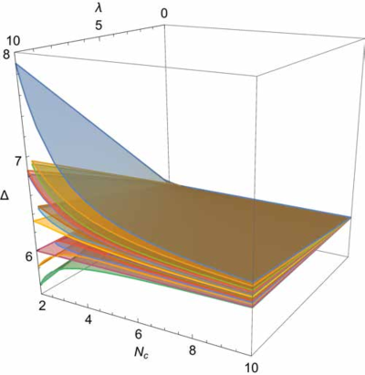
At large , the state with the smallest shown in Figure LABEL:fig:lam2, which is the double-trace operator for , has the lowest eigenvalue among all singlets at a fixed . Moreover, we observed that this lowest eigenstate does not become null for . The numerical values of the lowest eigenvalue in the singlets at are shown in Table 2 and Figure 4.
| 4 | 6 | 8 | 10 | |
|---|---|---|---|---|
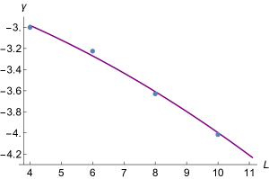
The results show that , the coefficient of the one-loop anomalous dimension, increases faster than linearly as increases. If we extrapolate this behavior at large , the lowest-energy state will have the dimension
| (5.8) |
neglecting for . At large , this expression hits the unitarity bound around very quickly. In other words, the operators with the anomalous dimension cannot be studied in the ’t Hooft limit.
The relation between the divergence of the lowest eigenvalue in and the pathological behavior of operators found in [8, 9] is unclear. The problem in the naïve planar limit has disappeared by including all non-planar corrections (i.e. by identifying the ground state of integrable spin chain with boundaries as a holomorphic-antiholomorphic operator). However, there is another operator whose dimension diverges in the large limit with all non-planar corrections included.
Let us recall that there are other situations where the integrability methods such as the generalized Lüscher formula or the mirror TBA disagree with perturbative field-theory calculation. Not all the disagreements are related to non-planar effects. One of the most puzzling examples is the single-particle state in the -deformed theory [71, 72]. The field theory calculation shows that this operator is protected owing to the so-called prewrapping effect. However, the TBA computation based on a naïve asymptotic Bethe Ansatz neglecting the prewrapping effect predicts a divergent answer. It is not known how to incorporate the prewrapping effect in the integrability methods.
5.2 Level-crossing and level-pairing
Below we regard one-loop dimensions as locally real analytic functions of , instead of collection of real numbers evaluated at integer values of . It allows us to keep track of each eigenstate from large to small .
5.2.1 Level-crossing
We ask the question when two operators have exactly the same one-loop dimensions at finite .
Consider the characteristic polynomial of the non-planar mixing matrix . This polynomial factorizes into
| (5.9) |
where is a prime polynomial over at generic values of .
The roots of different prime polynomials are unrelated, and nothing prevents the level-crossing. For example, at there exists an apparently non-BPS operator which is protected at any values of .131313It is known that this operator remains protected at two-loop order [62]. At we find two non-BPS operators whose anomalous dimensions are simple functions of . These energy levels do cross with the other energy levels.141414We use the words “energy level” and “one-loop anomalous dimension” interchangeably.
In contrast, the roots of the same prime polynomial rarely collide unless is small, which can be roughly explained as follows. The roots of the same prime polynomial come from a submatrix whose off-diagonal components are non-zero, and the non-zero off-diagonal components keep the eigenvalues separated.
Let us argue more accurately by writing down the condition that the one-loop dimensions of two operators coincide at finite . We denote the dilatation operator at and by and , respectively. We want to solve the eigenvalue equation at perturbatively around . The operator mixing equation can be written as
| (5.10) |
If we take the limit , only the states with contribute to the right-hand side. In particular, if the energy levels of two states are sufficiently close, the other energy levels are neglected. We denote the one-loop dimensions of the two states at by , respectively. The condition that these two states become degenerate at is given by
| (5.11) |
where . If is Hermitian, then the level-crossing is possible only if the off-diagonal components vanish. The off-diagonal components vanish, for example, when two states belong to different irreducible representations of the symmetry group of the model. This non-crossing rule is a famous statement by von Neumann and Wigner [50].
The matrix is not Hermitian in the non-planar mixing problem of SYM. Two roots of the same prime polynomial can collide and become a pair of complex conjugate roots. Of course, any gauge-invariant operators of SYM must have real dimensions, at least to all orders of perturbation in . It suggests that whenever two eigenvalues collide and become complex, the corresponding eigenvectors should be nullified by the finite reduction. As a corollary, the roots of a prime polynomial will never collide for .151515This fact can also be used as a consistency check on the computation of the non-planar mixing matrix.
A few remarks are in order. Since the levels repel each other, the energy levels are quite dense for , and the one-loop dimensions can change little as we vary as long as . Also, the expansion of the one-loop dimensions fails to converge at the points when complex roots show up.
5.2.2 Specifying branches
Let us consider the non-planar eigenvalue problem from a mathematical point of view.
The dimension of a physical operator is a root of the characteristic polynomial evaluated at integer points of . Since the polynomial is an analytic function of , the dimension can be analytically continued at any , which we call an eigenvalue curve. By keeping track of eigenvalue curves, we can see which finite eigenstate is connected to which of the large eigenstate.
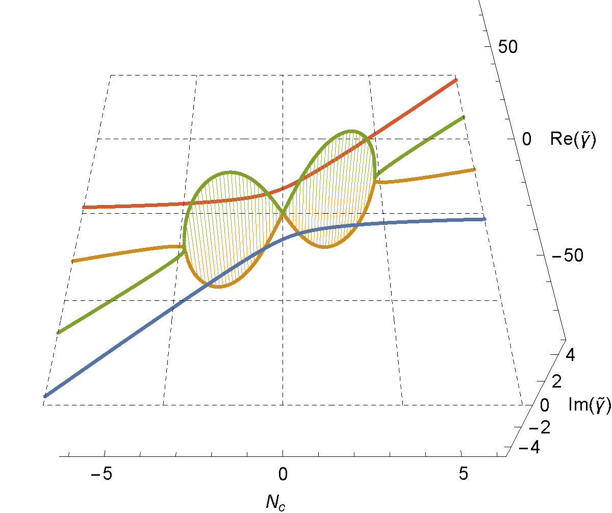
Not all large eigenstates can be extended to small . As decreases, a pair of adjacent energy levels collide and create a pair of complex conjugate energy levels. In other words, if we start from a small theory and increase , a new pair of states are created at finite . There also exists a pair-annihilation, where two adjacent energy levels collide as increases. The combination of pair-creations and pair-annihilations makes it quite non-trivial to keep track of eigenvalue curves as a function of . Some eigenvalue curves draw an S-shape trajectory on the plane via a pair-creation and pair-annihilation, as shown in Figure 5. Inside the S-shaped region, an eigenvalue curve is no longer a single-valued function of .
Mathematically, specifying an operator diagonalizing two-point functions of SYM, is equivalent to specifying one branch of the algebraic curve defined by the characteristic polynomial . We can define a branch of the algebraic curve algebraically or geometrically. Algebraically, a branch is a root of the characteristic polynomial , where is a single-valued function of . Geometrically, a branch is a connected component of the eigenvalue curves on the plane among the collection of eigenvalue curves. Although the two definitions are closely related, it turns out that an eigenvalue curve is not always a single-valued function of .161616Moreover, this definition depends on the choice of coordinates on the plane. In short, the geometric definition is more useful than the algebraic one at finite . Then, how many connected components are there? How precisely can we specify an operator of SYM?
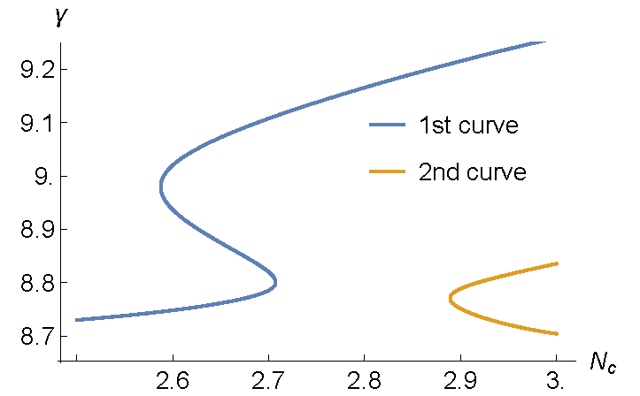
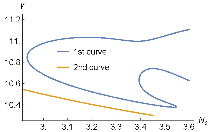
To answer this question, we must define the meaning of “connected”. It is convenient to exclude a point or points where almost all branches meet. In our definition of the one-loop dilatation operator , we should exclude the points and study the curve in the region . Then, each branch can be specified by prescribing their large behavior,
| (5.12) |
We define a connected curve by identifying the adjacent branches which collide at finite .
Alternatively, we can also use the rescaled eigenvalue . Then, the large dimensions can be read off from the asymptotic slope of the curves in plane, and we exclude the points .171717The large zero modes asymptotes to . We should also exclude these points. More importantly, the ’s stay finite around , and each eigenvalue curve can be smoothly extended to .
The reader may be upset because one cannot define gauge-invariant operators for . This difficulty can be circumvented by replacing gauge group with . The one-loop mixing matrix does not change if we modify to .181818We neglect the decoupling of for simplicity. The SYM scalar with gauge group should be extended to the scalar with gauge group by imposing . For a sufficiently large , the supergroup theory is not subject to any finite constraints and one gets non-unitary AdS/CFT correspondence realized by ghost D-branes [73, 74]. In this setup, the dilatation eigenvalues at negative are well-defined, and they can be complex due to the loss of unitarity.
Now let us have a closer look at the rescaled one-loop dimensions at negative .
If we take the limit , we should recover the spectrum of planar dilatation operator, neglecting the flipped sign. The invariance under can be understood as the invariance under the interchange of in the gauge group. Another explanation is that the ’t Hooft limit of theory is universal in the sense that one cannot discern if is positive or negative.191919The sign is important to distinguish the and SYM theory [75, 76, 77].
Let us give yet another proof that the dilatation spectra at are identical. From the block structure of the dilatation operator, one can show that the characteristic polynomial is compatible with the following symmetry:
| (5.13) |
To explain the block structure, let us take monomial multi-trace operators as a basis of the Hilbert space and collect the operators together according to their trace structure. The matrix elements of the dilatation operator within the same trace structure (i.e. block-diagonal parts) are of order , while those between different trace structures (i.e. block-off-diagonal parts) are of order . Now recalling the definition of the characteristic polynomial,
| (5.14) |
one finds that, for each , all terms come with an even power of . Hence the identity follows. Note that this identity does not imply that all eigenvalues are expanded in powers of , because there may be a pair of eigenvalues obeying .
In terms of the rescaled eigenvalues, the above identity induces an automorphism
| (5.15) |
which shows that the eigenvalue curves and their mirror-images are identical on the plane. In general, the automorphism relate different eigenvalue curves. To see this, consider the relation between the highest and the lowest eigenvalues.
| (5.16) |
Our data in Appendix B.2 shows that the outermost eigenvalues never collide with the adjacent eigenvalues, and remain real for real . Thus, the two energy levels are disjoint on the plane. Incidentally, the highest energy state in the sector is the product of Konishi operators, whose one-loop dimension at large behaves as .
Generally, by using we can group together the low-energy and high-energy eigenvalue curves as
| (5.17) |
Thus, the upper (or lower) half of the spectrum is redundant. We can throw away a half of the eigenvalue curves, or a half of the operators in SYM theory by using . We call it level-pairing. The level-pairing structure is evident from Figure 6, where we plotted the rescaled eigenvalues for at . The plots for is shown in Appendix B.2.3.
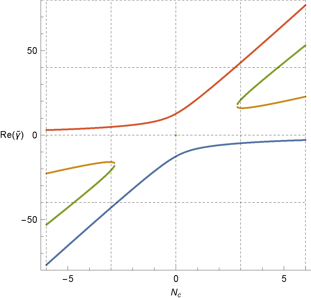
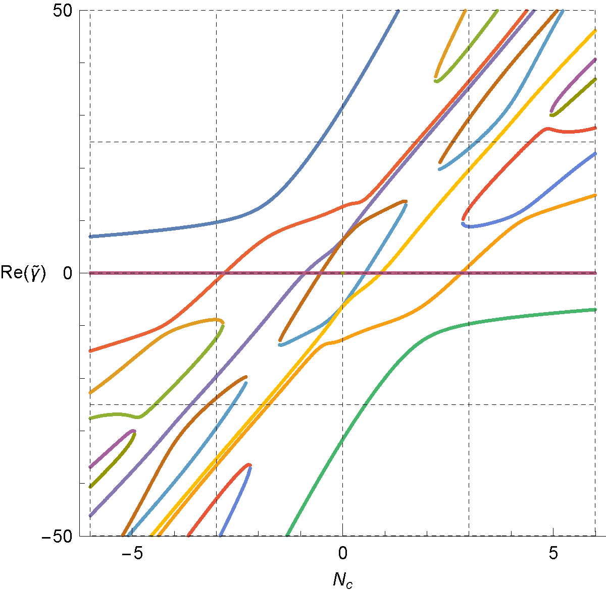
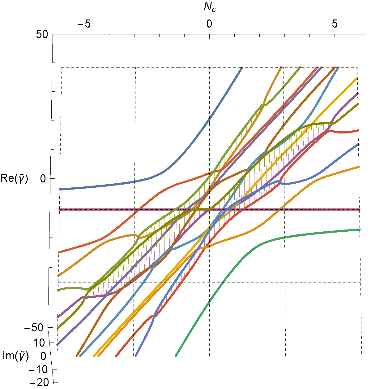
Here we list some properties of the level-pairing. First, maps a -protected states to itself, because is a straight line on the plane. Second, to find the level-pairing one must consider all multi-trace operators, even in the planar limit. Third, the level-pairing preserves charges.
The automorphism induces a non-trivial map between the conformal dimensions. It maps to . Then one needs to analytically continue to along the same eigenvalue curve to obtain . It is not easy to quantify the relation between and explicitly.
Let us make a few speculative comment about the automorphism . The symmetry should persist at higher orders in because this is a corollary of the large factorization (see [78] for a review). Then we can ask whether the level-pairing can be interpreted as certain duality on AdSS5 superstring in the planar limit. Such a transformation should act on multi-string states on AdSS5, and map a low-energy state to a high energy state. It should also satisfy other expected properties, namely to map a low-energy state to a high energy state, and a -protected state to itself with the same charges.
Since is a relation between multi-string states, a worldsheet duality (such as the worldsheet T-duality [79, 80, 81, 82]) cannot be the precise counterpart of . Nevertheless, it may happen that a collection of multi-string states can be described by a single-string coherent state if the number of strings is sufficiently large. For example, if the automorphism corresponds to the worldsheet T-duality, then the product of Konishi operator in the limit would be dual to a hoop-like string.202020An infinitely winding hoop string potentially suffers from two types of instability: corrections and corrections. The leading correction to the energy of a hoop string is complex [83], which represents the instability of a hoop shrinking into the north or south pole. It is likely that the correction is also complex. Since the hoop intersects with itself infinitely many times, each piece of the hoop can recombine itself to string bits without consuming energy. The resulting state may be dual to the Konishi product.
6 Discussion and Outlook
In this paper, we studied the spectrum of the non-planar one-loop dilatation operator among singlets by computing the matrix elements of operator mixing explicitly up to .
At large we considered the submixing problem, which concerns how the large degeneracy is lifted by corrections, and observed interesting patterns. First, the corrections to the dimensions of the large zero modes start appearing at the order . Second, the coefficient is always non-positive. Third, the operators with a different number of traces do not mix at large , and those with the same number of traces do mix. Fourth, the submixing density satisfies the projective commutation relations.
We have given some expressions of in terms of correlation functions and derived the submixing Hamiltonian. Using the correlator expression of , we have shown that is non-positive in the large approximation. We studied in detail -trace operators and the double-trace operator, which is the simplest operator to work because it does not submix the other large zero modes. We also estimated how depends on the operator length .
From the AdS/CFT point of view, the negative sign of can be interpreted as follows. Multi-trace operators can be regarded as multi-string states on AdSS5, and the product of BPS operators in SYM correspond to the product of BPS string states. In general a product of BPS states is not protected by supersymmetry. When multi-string states start interacting, they attract each other and form a bound state due to gravitational interaction. The negative sign should also be related to the causality constraint on the AdSS5 side [7]. To identify the precise relation, we need to clarify two issues. First, we studied singlets which are different from higher-spin operators of [7]. Second, we found operators which carry small positive anomalous dimensions at or higher.
When the rank of the gauge group is comparable to the operator length, we are studying determinant-like operators with all non-planar corrections taken into account. In AdS/CFT, the double-determinant operators should correspond to a pair of giant- and anti-giant-graviton D-branes. Such -brane configuration is unstable and should decay into the vacuum of AdSS5. At weak coupling, we find two interesting operators of whose behaviors are similar to those of the -brane system. The holomorphic-antiholomorphic operator can be regarded as non-planar completion of the double-determinant operator whose dimension is protected. The lowest-energy eigenstate in the sector has a negative anomalous dimension, which can be regarded as the non-planar ground state. We conjecture that the anomalous dimension of the lowest-energy state diverges to in the double scaling limit.212121It is not clear what the gravity dual of the lowest-energy state with is. The dual object might be a composite of another D-brane system, e.g. [84]. RS thanks Nadav Drukker for discussion on this point.
Furthermore, we have clarified the structure of level-crossing. When adjacent energy levels collide, the corresponding eigenstates should become null to prevent complex eigenvalues. We found it quite non-trivial to keep track of the operator dimensions as we vary . As a by-product, we discussed there is a natural pairing between different energy levels, particularly in the non-unitary theories.
Our methods are mostly based on brute-force computation, whose power is limited only to relatively small . The dimension of the mixing matrix grows factorially with respect to , and we encounter a challenging problem even numerically. It takes a long computational time to study the property of a huge matrix, and the results become less reliable due to the accumulation of numerical errors.
It is therefore important to look for another approach to the finite problem. In Section 4 we related the submixing to the four-point functions of (products of) BPS operators, which will be an interesting future direction. Examining the integrability in higher-point functions can be insightful, and rewriting the correlators in the Mellin space may also be useful [85, 86, 87].
Another promising approach to work on the finite physics is to exploit group representation theory. Operators can be labeled by a set of Young diagrams, and the operator mixing problem is neatly described by group theoretic quantities. Yet, the study of the operator mixing problem in the sector has not been very active so far because of the complexity caused by the flavor structure. The singlet sector is much simpler than the full sector. As we have seen in this paper, the singlet sector contains interesting physics that have not been observed in the sector. It would be one of the next directions to look closely into the sector at finite .
Acknowledgements
The authors acknowledge Agnese Bissi, Christoph Sieg, Gleb Arutyunov, Keisuke Okamura, Lionel Mason, Matthias Wilhelm, Luis Fernando Alday, Sanjaye Ramgoolam, Robert de Mello Koch, Tomek Lukowski for stimulating discussions. We also thank Nadav Drukker for detailed comments on the manuscript.
The work of RS is supported by Marie Curie Intra-European Fellowship of the European Community’s Seventh Framework Programme under the grant agreement number 327996. RS is RMCM of Kellogg College, University of Oxford.
We acknowledge useful conversations with workshop participants at the ESF and STFC supported workshop “Permutations and Gauge String duality”.
Appendix A Notation
Let us define real scalars of SYM by
| (A.1) |
where is the gauge group, and . As for , the symbol differentiates as
| (A.2) |
This rule can be used to compute the one-loop mixing matrix of theory as well by imposing the traceless condition when constructing a basis of operators. The splitting-and-joining rules follow straightforwardly:
| (A.3) |
The dilatation operator and conformal dimensions can be expanded in series of as222222The dimension of Konishi multiplet is .
| (A.4) |
The non-planar dilatation operators in the scalar sector at one-loop is
| (A.5) |
which commute with all generators. It also commutes with the projection operator to a union of eigenspaces ,
| (A.6) |
The first term of acts on multi-trace operators as
| (A.7) | ||||
| (A.8) | ||||
| (A.9) | ||||
| (A.10) |
and the second term as
| (A.11) | ||||
| (A.12) | ||||
| (A.13) | ||||
| (A.14) |
A.1 Notation for operator mixing
To highlight the structure of the non-planar operator mixing, we introduce a formal parameter so that the global symmetry becomes . The SYM corresponds to . There can be several ways to define the dilatation operator at general , but the difference is not much important at the fully non-planar level. We use the simplest generalization; namely the operator identical to except that the flavor indices run .232323Another possible generalization is which is integrable at large [88, 89, 32].
The matrix of operator mixing is defined as follows. We use monomial multi-trace operators as the basis, and denote them by . By applying the one-loop dilatation to them, we obtain the mixing matrix
| (A.15) |
Then we look for the eigenvector of the form , which implies . Note that this mixing matrix is the transpose of , and in Mathematica the eigenvectors are given by Eigenvectors[Transpose@M].Table[O[i],{i,d}]. The matrix elements of operator submixing will be defined in the same way, namely
| (A.16) |
Explicit matrix elements are computed via .
Appendix B Foundations of finite calculation
B.1 Finite reduction
When the rank of the gauge group is smaller than the operator length, gauge-invariant operators become linearly dependent. This is a well-known phenomenon, and the linear relations are called finite constraints.242424This is a non-perturbative effect on the string theory side, and called the stringy exclusion principle [90]. Any finite constraints are written as the identity for an antisymmetric tensor
| (B.1) |
As decreases, the dimension of the Hilbert space of states shrinks by finite reduction.
The two-point functions at tree level can be diagonalized at any by using group-theoretical bases [10, 13, 12, 17]. In these bases, finite constraints are typically written as , where is the number of rows of a Young diagram . A set of finite constraints in the scalar sector was given in [17]. In general there are several ways to express the finite constraints in a given sector. (This is the same as that there are several orthogonal bases in a sector.) The reason can be clarified from the existence of some sets of conserved charges at tree level [63].
At the loop level, there is no freedom in choosing the basis in which the two-point functions are orthonormal, except for degenerate cases. Still, the finite constraints reduce the dimension of the Hilbert space of gauge-invariant operators. When the finite constraints are imposed, we should find either (i) the eigenvalues remain unchanged, or (ii) the eigenvector becomes null. Written explicitly, this means
| (B.2) |
where is the eigenstate subject to the finite constraints.
Let us make a few remarks. First, if an eigenvector becomes null, all correlators involving also vanish.252525See [91] for an example. Second, if an eigenvector becomes null at , then it remains null for , as follows from .
A simple way to determine which eigenvector survives at finite is to substitute real traceless matrices to the fields . In other words, we regard multi-trace operators as -invariant polynomials of the matrix elements . When decreases by one, we remove the last row and column of the matrix elements. Schematically, this can be depicted as removing gray region of the following matrix:
| (B.3) |
By exploiting this idea, one can associate a Young diagram to each eigenstate as follows. Instead of removing the last row and column, we can rescale the entries in the last column and the last row by . The diagonal element are rescaled by . Then we measure how an eigenstate scales in the limit; as . We can continue this procedure as
| (B.4) |
until . This assigns to each eigenstate a sequence of integers which is a partition of .
The finite - constraints put restrictions on the matrix elements of non-planar operator mixing. Let be the space of the -invariant polynomials of which vanish for . In other words, is the smallest integer satisfying for all . Each is closed under the dilatation operator. However, the mixing matrices are generally not block diagonal on the basis of . To see it, expand the eigenvector which becomes null at as
| (B.5) |
The null condition gives . Since the coefficients are non-trivial functions of , they do not identically vanish.
That said, the same reasoning allows us to remove some elements of the mixing matrix. If we use monomial multi-traces as the basis of operators, then the elements of mixing matrix are at most linear in ; see -. This property remains unchanged unless we rotate the basis by a -dependent matrix. Then, the condition implies , which excludes off-diagonal elements from to for .
B.2 Spectral data
We summarize the basic properties of the finite spectrum, and the spectral data of one-loop anomalous dimensions for the scalar singlet operators at finite with length . These results are obtained by explicit computation using Mathematica. The data include plots of the finite spectrum, the submixing matrix and the basis of operators. The eigenvalues of submixing matrices are given at general values of for .
B.2.1
There are four singlets at length .
The matrix elements and operator basis for general are given by262626In a computer-friendly format, is
{{4,-2,-2*Nf/Nc,2/Nc},{-2,3+Nf,-2/Nc,Nc^(-1)+Nf/Nc},{2/Nc-2*Nf/Nc,-2/Nc+2*Nf/Nc,0,2},{-12/Nc,12/Nc,0,2*Nf}}
One can derive submixing matrix elements and various finite plots from this data as presented below.
| (B.6) |
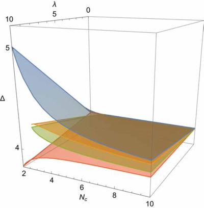
which is consistent with [61] at . The spectrum is shown in Figure 7. The eigenvalue curve is drawn by keeping track of the large eigenvalues down to small as long as they remain real-valued. The complex eigenvalues are not shown, and some of them have null eigenvectors. Whenever the complex eigenvalues show up, the corresponding eigenvectors become null [95].

There is one large zero mode, so the submixing matrix is one-dimensional:
| (B.7) |
where is the symmetric traceless tensor defined in . The corrections to this operator for general are given by
| (B.8) |
B.2.2
There are fifteen singlets at length . The mixing matrix and operator basis for general are given by
{{6,3,-6,0,0,(3*Nf)/Nc,3/Nc,-6/Nc,0,6/Nc-(3*Nf)/Nc,3/Nc,-6/Nc,0,0,0},
{0,4+Nf,0,-4,2,2/Nc,2/Nc+(2*Nf)/Nc,-6/Nc,0,-4/Nc,3/Nc-Nf/Nc,2/Nc,0,0,0},
{-2,1,6,-2,0,-6/Nc+Nf/Nc,Nc^(-1),4/Nc-(2*Nf)/Nc,2/Nc,-6/Nc,2/Nc+Nf/Nc,4/Nc-Nf/Nc,0,0,0},
{0,-3/2,-2,6+Nf/2,0,(-2*Nf)/Nc,3/(2*Nc),-2/Nc,2/Nc+Nf/(2*Nc),2/Nc,Nc^(-1)+Nf/Nc,-4/Nc,0,0,0},
{0,3/2,0,-3,3+(3*Nf)/2,-6/Nc,15/(2*Nc)+(3*Nf)/(2*Nc),0,-3/Nc,0,0,0,0,0,0},
{2/Nc,2/Nc+Nf/Nc,-4/Nc,(-2*Nf)/Nc,Nf/Nc,3+Nf/2,3/2,-2,0,0,0,0,-2/Nc,Nc^(-1)+Nf/(2*Nc),1/(2*Nc)},
{0,12/Nc,0,-24/Nc,12/Nc,0,3+2*Nf,0,-2,0,0,0,0,-2/Nc,Nc^(-1)+Nf/Nc},
{-4/Nc,-2/Nc,6/Nc-(2*Nf)/Nc,-2/Nc+(2*Nf)/Nc,2/Nc,-2,0,4,1,0,0,0,-(Nf/Nc),Nc^(-1),0},
{0,0,-24/Nc,24/Nc,0,0,-2,0,4+Nf,0,0,0,0,(-2*Nf)/Nc,2/Nc},
{6/Nc-(3*Nf)/Nc,6/Nc,-12/Nc,6/Nc+(3*Nf)/Nc,-6/Nc,0,0,0,0,6,3,-6,0,0,0},
{-4/Nc,-2/Nc-Nf/Nc,-4/Nc,4/Nc,6/Nc+Nf/Nc,0,0,0,0,0,2+Nf,0,0,0,0},
{-6/Nc,(3*Nf)/Nc,12/Nc-(3*Nf)/Nc,-6/Nc,0,0,0,0,0,-6,3,6,0,0,0},
{0,0,0,0,0,-6/Nc+(3*Nf)/Nc,3/Nc,6/Nc-(3*Nf)/Nc,-3/Nc,0,0,0,0,3,0},
{0,0,0,0,0,24/Nc,-2/Nc+(2*Nf)/Nc,-24/Nc,2/Nc-(2*Nf)/Nc,0,0,0,0,Nf,2},
{0,0,0,0,0,0,36/Nc,0,-36/Nc,0,0,0,0,0,3*Nf}}
and
| (B.9) |
The spectrum is shown in Figure 8. This mixing matrix is consistent with [62], which can be shown by computing the characteristic polynomial and substituting .
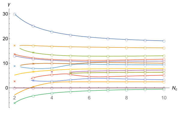
There are two large zero modes. The submixing matrix for general is given by
| (B.10) |
The double- and triple-trace zero modes do not submix. At , the double-trace mode has and the triple-trace mode has precisely zero dimension for any [62].
We also studied operators other than singlets. No negative modes () are found in the sector at , and the lowest eigenvalue in the sector at is same as the lowest eigenvalue of the singlets.
B.2.3
There are 71 singlets at length . The mixing matrix and operator basis for general are given by
{{6+Nf,-4,0,-2,0,0,0,0,0,0,0,0,2,0,0,0,0,1,4/Nc,Nc^(-1),2/Nc+(2*Nf)/Nc,-4/Nc,-4/Nc,-2/Nc,0,0,0,0,0,0,0,Nc^(-1),10/Nc,8/Nc-(2*Nf)/Nc,-8/Nc,-6/Nc,0,-2/Nc,0,5/Nc,Nf/Nc,2/Nc,-4/Nc,0,-4/Nc,0,0,0,0,0,0,0,0,0,0,0,0,0,0,0,0,0,0,0,0,0,0,0,0,0,0},
{-3/2,7+Nf/2,0,0,0,-1,0,0,0,-1,0,0,0,0,0,-2,2,0,-Nc^(-1),2/Nc-(2*Nf)/Nc,2/Nc,Nc^(-1),Nc^(-1),0,2/Nc+Nf/Nc,0,0,-6/Nc,0,0,0,0,-4/Nc,2/Nc+Nf/Nc,6/Nc,0,2/Nc-Nf/Nc,0,-6/Nc,Nc^(-1),-1/(2*Nc),0,4/Nc,Nc^(-1)+Nf/(2*Nc),-2/Nc,0,-2/Nc,-2/Nc,0,0,0,0,0,0,0,0,0,0,0,0,0,0,0,0,0,0,0,0,0,0,0},
{0,0,8,4,0,0,0,0,-8,0,0,0,0,0,0,0,0,0,-8/Nc,4/Nc,0,0,0,8/Nc,4/Nc,-8/Nc,0,0,0,0,0,0,-8/Nc,4/Nc,8/Nc+(4*Nf)/Nc,0,0,0,-8/Nc,0,0,0,0,0,-8/Nc,8/Nc-(4*Nf)/Nc,4/Nc,0,0,0,0,0,0,0,0,0,0,0,0,0,0,0,0,0,0,0,0,0,0,0,0},
{-2,0,0,6+Nf,0,-2,2,0,0,-2,0,0,0,0,0,0,0,1,4/Nc,Nc^(-1),Nc^(-1),0,0,-2/Nc,4/Nc+Nf/Nc,0,0,0,-8/Nc,0,0,-Nc^(-1),-8/Nc,-2/Nc,10/Nc,0,0,4/Nc+(2*Nf)/Nc,-6/Nc,0,Nc^(-1),0,-4/Nc,0,2/Nc,-4/Nc,7/Nc-(2*Nf)/Nc,0,0,0,0,0,0,0,0,0,0,0,0,0,0,0,0,0,0,0,0,0,0,0,0},
{0,0,0,0,8,-1,2,0,0,-1,-4,0,0,0,0,0,0,0,2/Nc,-4/Nc,0,-Nc^(-1),-Nc^(-1),0,2/Nc,2/Nc-(2*Nf)/Nc,2/Nc,0,0,0,0,0,-2/Nc+Nf/Nc,Nc^(-1)+(2*Nf)/Nc,0,4/Nc,2/Nc,0,-8/Nc,2/Nc,0,4/Nc-Nf/Nc,-2/Nc,0,-4/Nc,-2/Nc,0,4/Nc-Nf/Nc,0,0,0,0,0,0,0,0,0,0,0,0,0,0,0,0,0,0,0,0,0,0,0},
{0,-1,0,-1/2,-1,7+Nf/2,-1/2,0,0,1/2,0,-2,1,-1,1/2,0,1/2,0,-Nc^(-1)+Nf/(2*Nc),1/(2*Nc),1/(2*Nc),1/(2*Nc)-Nf/Nc,3/(2*Nc),-Nc^(-1),Nc^(-1),0,2/Nc+Nf/(2*Nc),-Nc^(-1),-3/(2*Nc),-2/Nc,0,1/(2*Nc),6/Nc-Nf/Nc,1/(2*Nc)+Nf/(2*Nc),-6/Nc,-2/Nc,Nc^(-1),2/Nc+Nf/Nc,-2/Nc,Nc^(-1)+Nf/(2*Nc),0,-2/Nc,3/Nc-Nf/Nc,1/(2*Nc),0,0,-Nc^(-1),-Nc^(-1),0,0,0,0,0,0,0,0,0,0,0,0,0,0,0,0,0,0,0,0,0,0,0},
{0,0,0,1,0,-1,6+Nf,0,0,-1,0,0,-1,0,-2,0,1,0,-3/Nc,0,-Nc^(-1),-1/(2*Nc),-1/(2*Nc),0,4/Nc+Nf/Nc,-3/Nc,0,0,3/Nc-Nf/Nc,0,0,Nc^(-1),-8/Nc,9/(2*Nc),4/Nc,2/Nc,-3/Nc,3/Nc+(3*Nf)/(2*Nc),-4/Nc,5/Nc-Nf/Nc,Nc^(-1),0,3/Nc,0,0,0,-5/Nc,-3/Nc,0,0,0,0,0,0,0,0,0,0,0,0,0,0,0,0,0,0,0,0,0,0,0},
{2,0,0,0,0,0,0,8,-4,0,0,2,0,-4,0,0,0,0,0,(2*Nf)/Nc,2/Nc,0,0,0,0,-4/Nc,0,-8/Nc,2/Nc,4/Nc,2/Nc,0,-4/Nc,0,-4/Nc,16/Nc-(4*Nf)/Nc,4/Nc,0,-8/Nc,2/Nc+(2*Nf)/Nc,0,4/Nc,0,0,-8/Nc,0,0,0,0,0,0,0,0,0,0,0,0,0,0,0,0,0,0,0,0,0,0,0,0,0,0},
{1,0,-2,1,0,1,0,-2,8,1,-4,0,0,0,0,0,0,0,-2/Nc,Nc^(-1)+Nf/Nc,Nc^(-1),-3/Nc,-3/Nc,2/Nc,Nc^(-1),0,2/Nc,4/Nc,0,-4/Nc,0,0,4/Nc+(2*Nf)/Nc,0,-6/Nc,-6/Nc,2/Nc,2/Nc,4/Nc-(2*Nf)/Nc,Nc^(-1),0,-2/Nc,2/Nc,0,2/Nc-(2*Nf)/Nc,-2/Nc,Nf/Nc,0,0,0,0,0,0,0,0,0,0,0,0,0,0,0,0,0,0,0,0,0,0,0,0},
{0,-1,0,-1/2,-1,1/2,-1/2,0,0,7+Nf/2,0,-2,1,-1,1/2,0,1/2,0,-Nc^(-1)+Nf/(2*Nc),1/(2*Nc),1/(2*Nc),3/(2*Nc),1/(2*Nc)-Nf/Nc,-Nc^(-1),Nc^(-1),0,2/Nc+Nf/(2*Nc),-Nc^(-1),-3/(2*Nc),-2/Nc,0,1/(2*Nc),6/Nc-Nf/Nc,1/(2*Nc)+Nf/(2*Nc),-6/Nc,-2/Nc,Nc^(-1),2/Nc+Nf/Nc,-2/Nc,Nc^(-1)+Nf/(2*Nc),0,-2/Nc,3/Nc-Nf/Nc,1/(2*Nc),0,0,-Nc^(-1),-Nc^(-1),0,0,0,0,0,0,0,0,0,0,0,0,0,0,0,0,0,0,0,0,0,0,0},
{0,1,0,0,-2,1/2,1,0,-2,1/2,8,-1,0,-2,0,0,0,0,Nc^(-1),-3/Nc,0,-3/(2*Nc)+Nf/(2*Nc),-3/(2*Nc)+Nf/(2*Nc),2/Nc,2/Nc,-Nc^(-1),Nc^(-1),-2/Nc,0,2/Nc-Nf/Nc,Nc^(-1),0,-2/Nc,5/(2*Nc),Nf/Nc,-2/Nc,2/Nc+Nf/(2*Nc),0,(-2*Nf)/Nc,-2/Nc,0,0,3/Nc+Nf/Nc,0,-(Nf/Nc),-2/Nc,2/Nc,-Nc^(-1),0,0,0,0,0,0,0,0,0,0,0,0,0,0,0,0,0,0,0,0,0,0,0},
{1/2,0,0,0,0,-2,0,0,0,-2,-2,8+Nf/2,2,0,-1,0,0,0,Nc^(-1)+Nf/Nc,3/Nc,2/Nc,-2/Nc,-2/Nc,-2/Nc,0,0,-Nc^(-1),-4/Nc,Nf/(2*Nc),0,2/Nc+Nf/(2*Nc),Nc^(-1),-6/Nc,Nc^(-1),6/Nc-(3*Nf)/Nc,-4/Nc,4/Nc,0,2/Nc,2/Nc+Nf/(2*Nc),1/(2*Nc),0,-4/Nc,0,-4/Nc,2/Nc,2/Nc+Nf/Nc,0,0,0,0,0,0,0,0,0,0,0,0,0,0,0,0,0,0,0,0,0,0,0,0},
{1/2,-1,0,0,0,0,-2,0,0,0,0,0,6+(3*Nf)/2,0,0,0,-2,1,Nc^(-1),-2/Nc,4/Nc+Nf/Nc,-3/Nc,-3/Nc,0,-2/Nc,0,0,0,Nc^(-1),0,0,2/Nc+Nf/Nc,4/Nc,Nc^(-1),-8/Nc,0,-2/Nc,6/Nc-Nf/Nc,0,-Nc^(-1),5/(2*Nc)+Nf/(2*Nc),0,-6/Nc,-Nc^(-1),0,0,5/Nc,0,0,0,0,0,0,0,0,0,0,0,0,0,0,0,0,0,0,0,0,0,0,0,0},
{0,1,0,0,0,-1/2,0,-1,0,-1/2,-2,1/2,0,8,-1/2,-1,0,0,0,-Nc^(-1),0,-1/(2*Nc)+Nf/(2*Nc),-1/(2*Nc)+Nf/(2*Nc),-4/Nc,Nc^(-1),0,5/(2*Nc),4/Nc-(2*Nf)/Nc,Nc^(-1),-2/Nc,1/(2*Nc),0,-Nc^(-1),Nc^(-1),-Nc^(-1),2/Nc-(2*Nf)/Nc,3/Nc+Nf/Nc,Nc^(-1),-4/Nc,3/(2*Nc),0,-Nc^(-1),-Nc^(-1)+Nf/Nc,0,0,-Nc^(-1),-3/(2*Nc),2/Nc,0,0,0,0,0,0,0,0,0,0,0,0,0,0,0,0,0,0,0,0,0,0,0},
{1/2,0,0,0,0,1/2,-1,0,0,1/2,0,-1,0,-2,7+Nf/2,0,-1,0,-Nc^(-1),-2/Nc,Nc^(-1),3/Nc-Nf/Nc,3/Nc-Nf/Nc,-4/Nc,2/Nc,-2/Nc,2/Nc+Nf/(2*Nc),0,Nf/(2*Nc),0,-Nc^(-1),0,4/Nc-Nf/Nc,Nf/Nc,-6/Nc,-8/Nc,2/Nc,4/Nc,4/Nc,-5/Nc,1/(2*Nc),0,2/Nc,0,0,0,2/Nc+Nf/(2*Nc),0,0,0,0,0,0,0,0,0,0,0,0,0,0,0,0,0,0,0,0,0,0,0,0},
{0,-3,0,0,0,0,0,0,0,0,0,0,0,-2,1,8,0,0,0,0,0,Nc^(-1),Nc^(-1),(-4*Nf)/Nc,4/Nc,2/Nc,Nc^(-1),-4/Nc,Nc^(-1),-2/Nc,0,0,0,2/Nc,0,-8/Nc,(2*Nf)/Nc,0,4/Nc,0,0,-2/Nc,-2/Nc,-Nc^(-1),-2/Nc,2/Nc,Nc^(-1),2/Nc,2/Nc,0,0,0,0,0,0,0,0,0,0,0,0,0,0,0,0,0,0,0,0,0,0},
{0,1/2,0,0,0,0,1,0,0,0,0,0,-3/2,0,-2,-1,6+Nf,0,3/Nc-(2*Nf)/Nc,-4/Nc,0,-Nc^(-1),-Nc^(-1),-2/Nc,5/Nc+Nf/Nc,0,-2/Nc,0,Nc^(-1),0,0,2/Nc,-8/Nc,3/Nc,4/Nc,0,-4/Nc,4/Nc+Nf/Nc,0,-3/Nc,-1/(2*Nc),0,-2/Nc,7/(2*Nc),0,0,3/Nc,0,-Nc^(-1),0,0,0,0,0,0,0,0,0,0,0,0,0,0,0,0,0,0,0,0,0,0},
{0,0,0,0,0,0,0,0,0,0,0,0,2,0,0,0,-4,4+2*Nf,-8/Nc,0,2/Nc,0,0,0,-4/Nc,0,0,0,0,0,0,8/Nc+(2*Nf)/Nc,0,-12/Nc,0,0,0,12/Nc,0,4/Nc,8/Nc,0,0,-4/Nc,0,0,-8/Nc,0,0,0,0,0,0,0,0,0,0,0,0,0,0,0,0,0,0,0,0,0,0,0,0},
{3/Nc,-6/Nc,0,3/Nc,0,-Nc^(-1),-4/Nc,0,0,-Nc^(-1),0,4/Nc,4/Nc+Nf/Nc,0,-6/Nc,0,5/Nc-(2*Nf)/Nc,-Nc^(-1)+Nf/Nc,3+Nf,1/2,0,-1,-1,-1,0,0,0,0,1,0,0,3/2,0,0,0,0,0,0,0,0,0,0,0,0,0,0,0,0,0,5/Nc+Nf/Nc,5/(2*Nc),-2/Nc,-4/Nc,-2/Nc,-Nc^(-1),0,0,1/(2*Nc),0,2/Nc,-2/Nc,0,0,0,0,0,0,0,0,0,0},
{Nc^(-1)+Nf/Nc,4/Nc-(2*Nf)/Nc,0,-4/Nc,0,1/(2*Nc),Nc^(-1),2/Nc,2/Nc,1/(2*Nc),-6/Nc,6/Nc,Nf/Nc,-6/Nc,-Nc^(-1),0,-Nc^(-1),Nc^(-1),2,4+Nf/2,3/2,-1,-1,-2,0,0,0,0,0,0,0,0,0,0,0,0,0,0,0,0,0,0,0,0,0,0,0,0,0,2/Nc+Nf/Nc,Nf/(2*Nc),0,2/Nc,0,0,-4/Nc,-2/Nc,1/(2*Nc),0,Nc^(-1),2/Nc-Nf/Nc,0,2/Nc,0,-4/Nc,0,0,0,0,0,0},
{12/Nc,-24/Nc,0,0,0,0,-12/Nc,0,0,0,0,0,24/Nc,0,0,0,0,0,0,0,4+2*Nf,0,0,0,-4,0,0,0,0,0,0,2,0,0,0,0,0,0,0,0,0,0,0,0,0,0,0,0,0,2/Nc,0,0,0,-6/Nc,0,0,0,2/Nc+(2*Nf)/Nc,0,0,0,2/Nc,0,-4/Nc,0,3/Nc-Nf/Nc,0,0,0,0,0},
{-3/(2*Nc),3/(2*Nc),0,1/(2*Nc)+Nf/(2*Nc),-3/Nc,4/Nc-Nf/Nc,1/(2*Nc)+Nf/Nc,0,0,5/(2*Nc),2/Nc,-4/Nc,1/(2*Nc),-Nc^(-1),1/(2*Nc)-Nf/Nc,-3/Nc,-1/(2*Nc)+Nf/(2*Nc),Nc^(-1),0,-1,0,5+Nf/2,1,0,1,-1,0,-1,-1/2,0,0,0,0,0,0,0,0,0,0,0,0,0,0,0,0,0,0,0,0,0,1/(2*Nc),-2/Nc,2/Nc-Nf/Nc,2/Nc+Nf/(2*Nc),0,0,-2/Nc,0,0,Nc^(-1)+Nf/(2*Nc),0,0,-4/Nc,0,2/Nc,1/(2*Nc),0,0,0,0,0},
{-3/(2*Nc),3/(2*Nc),0,1/(2*Nc)+Nf/(2*Nc),-3/Nc,5/(2*Nc),1/(2*Nc)+Nf/Nc,0,0,4/Nc-Nf/Nc,2/Nc,-4/Nc,1/(2*Nc),-Nc^(-1),1/(2*Nc)-Nf/Nc,-3/Nc,-1/(2*Nc)+Nf/(2*Nc),Nc^(-1),0,-1,0,1,5+Nf/2,0,1,-1,0,-1,-1/2,0,0,0,0,0,0,0,0,0,0,0,0,0,0,0,0,0,0,0,0,0,1/(2*Nc),-2/Nc,2/Nc-Nf/Nc,2/Nc+Nf/(2*Nc),0,0,-2/Nc,0,0,Nc^(-1)+Nf/(2*Nc),0,0,-4/Nc,0,2/Nc,1/(2*Nc),0,0,0,0,0},
{0,2/Nc+Nf/Nc,2/Nc,Nc^(-1),2/Nc,-3/(2*Nc),Nc^(-1),0,-2/Nc,-3/(2*Nc),0,0,0,-6/Nc,Nc^(-1),2/Nc-(2*Nf)/Nc,Nf/Nc,0,0,-3/2,0,1/2,1/2,5,3/2,0,0,-2,0,0,0,0,0,0,0,0,0,0,0,0,0,0,0,0,0,0,0,0,0,2/Nc,-1/(2*Nc),(-2*Nf)/Nc,0,Nc^(-1),Nc^(-1),-2/Nc,0,0,1/(2*Nc),Nc^(-1),Nf/Nc,0,-4/Nc,0,2/Nc,0,0,0,0,0,0},
{0,6/Nc,0,6/Nc,0,-6/Nc,12/Nc,0,0,-6/Nc,0,0,0,0,-12/Nc,-12/Nc,12/Nc,0,0,0,-3/2,0,0,0,6+(3*Nf)/2,0,-2,0,0,0,0,0,0,0,0,0,0,0,0,0,0,0,0,0,0,0,0,0,0,(-2*Nf)/Nc,0,0,0,-2/Nc,0,0,0,3/(2*Nc),2/Nc+Nf/(2*Nc),0,0,-4/Nc,0,2/Nc,0,Nc^(-1)+Nf/Nc,0,0,0,0,0},
{0,-6/Nc,0,0,6/Nc-(2*Nf)/Nc,Nc^(-1)+Nf/Nc,2/Nc,0,0,Nc^(-1)+Nf/Nc,-8/Nc,0,0,4/Nc,-4/Nc,0,4/Nc,0,0,0,0,-1,-1,0,0,6,1,0,1,-2,0,0,0,0,0,0,0,0,0,0,0,0,0,0,0,0,0,0,0,2/Nc,0,-4/Nc,-2/Nc,2/Nc,0,0,4/Nc-(2*Nf)/Nc,0,0,Nf/Nc,2/Nc,-Nc^(-1),4/Nc,0,-6/Nc,0,0,0,0,0,0},
{0,0,0,0,-12/Nc,12/Nc,0,0,0,12/Nc,0,0,0,-24/Nc,12/Nc,0,0,0,0,0,1,0,0,0,-2,0,6+Nf,0,0,0,-2,0,0,0,0,0,0,0,0,0,0,0,0,0,0,0,0,0,0,-6/Nc+Nf/Nc,0,0,0,4/Nc-(2*Nf)/Nc,0,0,0,Nc^(-1),2/Nc,0,0,4/Nc-Nf/Nc,0,-6/Nc,0,2/Nc+Nf/Nc,0,0,0,0,0},
{Nc^(-1),-Nc^(-1),-2/Nc,Nc^(-1),-2/Nc,-1/(2*Nc)+Nf/(2*Nc),-Nc^(-1),-4/Nc,4/Nc,-1/(2*Nc)+Nf/(2*Nc),0,-2/Nc,Nc^(-1),6/Nc-(2*Nf)/Nc,Nc^(-1)+Nf/Nc,-2/Nc,Nc^(-1),0,0,1,0,0,0,-2,0,0,1,6,0,-2,0,0,0,0,0,0,0,0,0,0,0,0,0,0,0,0,0,0,0,Nc^(-1),0,-4/Nc,-2/Nc+Nf/Nc,Nc^(-1),0,2/Nc-Nf/Nc,2/Nc,0,0,Nc^(-1),Nc^(-1)+Nf/(2*Nc),0,4/Nc-Nf/Nc,0,-6/Nc,1/(2*Nc),0,0,0,0,0},
{0,0,0,2/Nc,0,-6/Nc,8/Nc-(2*Nf)/Nc,0,0,-6/Nc,0,4/Nc,4/Nc+(2*Nf)/Nc,0,4/Nc,0,-12/Nc,2/Nc,2,0,1,-2,-2,0,0,0,0,0,4+Nf,0,0,0,0,0,0,0,0,0,0,0,0,0,0,0,0,0,0,0,0,2/Nc+Nf/Nc,0,0,2/Nc,0,0,0,-6/Nc,Nc^(-1),0,3/Nc,0,0,2/Nc,0,-4/Nc,-Nc^(-1),0,0,0,0,0},
{2/Nc,-4/Nc,0,0,0,-3/Nc,0,4/Nc,-8/Nc,-3/Nc,6/Nc-(2*Nf)/Nc,2/Nc+(2*Nf)/Nc,2/Nc,0,2/Nc,0,0,0,0,2,0,0,0,0,0,-2,0,-4,1,6,1,0,0,0,0,0,0,0,0,0,0,0,0,0,0,0,0,0,0,4/Nc,0,0,(2*Nf)/Nc,0,0,-4/Nc,-2/Nc,0,0,Nc^(-1),2/Nc,0,-6/Nc,-Nc^(-1),6/Nc-(2*Nf)/Nc,0,0,0,0,0,0},
{0,0,0,0,0,0,0,0,0,0,-36/Nc,36/Nc,0,0,0,0,0,0,0,0,3,0,0,0,0,0,-6,0,0,0,6+Nf,0,0,0,0,0,0,0,0,0,0,0,0,0,0,0,0,0,0,(3*Nf)/Nc,0,0,0,-6/Nc,0,0,0,3/Nc,0,0,0,-6/Nc,0,6/Nc-(3*Nf)/Nc,0,3/Nc,0,0,0,0,0},
{0,0,0,0,0,0,0,0,0,0,0,0,18/Nc,0,0,0,-36/Nc,18/Nc,0,0,3/2,0,0,0,-3,0,0,0,0,0,0,3+(5*Nf)/2,0,0,0,0,0,0,0,0,0,0,0,0,0,0,0,0,0,-6/Nc,0,0,0,0,0,0,0,15/(2*Nc)+(3*Nf)/(2*Nc),-3/Nc,0,0,0,0,0,0,0,0,0,0,0,0},
{3/Nc+Nf/Nc,-4/Nc,0,0,0,11/(2*Nc)-Nf/Nc,-4/Nc,-4/Nc,4/Nc,11/(2*Nc)-Nf/Nc,-4/Nc,-6/Nc,Nc^(-1)+(2*Nf)/Nc,-2/Nc,5/Nc-Nf/Nc,0,0,0,0,0,0,0,0,0,0,0,0,0,0,0,0,0,8+Nf/2,1/2,-5,-2,0,2,0,0,0,0,0,0,0,0,0,0,0,0,0,0,0,0,0,0,0,0,0,-Nc^(-1),2/Nc,2/Nc+Nf/(2*Nc),0,-Nc^(-1),-4/Nc,3/(2*Nc),0,0,0,0,0},
{Nc^(-1)-Nf/Nc,-Nc^(-1),0,-Nc^(-1),2/Nc,-1/(2*Nc),3/Nc,0,0,-1/(2*Nc),-4/Nc,-4/Nc,Nc^(-1)+Nf/Nc,-6/Nc,3/Nc,-2/Nc,7/Nc,2/Nc,0,0,0,0,0,0,0,0,0,0,0,0,0,0,0,5+Nf,0,0,-2,0,0,0,0,0,0,0,0,0,0,0,0,0,0,0,0,0,0,0,0,0,0,2/Nc-Nf/Nc,-4/Nc,0,0,0,0,2/Nc+Nf/Nc,0,0,0,0,0},
{2/Nc,5/Nc,2/Nc,3/Nc+Nf/Nc,0,-5/Nc,3/Nc+Nf/Nc,0,-4/Nc,-5/Nc,2/Nc,6/Nc-(3*Nf)/Nc,0,-4/Nc,-4/Nc,-2/Nc,3/Nc+Nf/Nc,-2/Nc,0,0,0,0,0,0,0,0,0,0,0,0,0,0,-5,1/2,8+Nf/2,0,0,2,-2,0,0,0,0,0,0,0,0,0,0,0,0,0,0,0,0,0,0,0,0,-Nc^(-1),2/Nc,-Nc^(-1),-4/Nc,2/Nc+Nf/(2*Nc),0,3/(2*Nc),0,0,0,0,0},
{-Nc^(-1),3/Nc+Nf/Nc,0,-2/Nc,2/Nc,-Nc^(-1)+Nf/(2*Nc),3/Nc+Nf/Nc,4/Nc-Nf/Nc,-4/Nc,-Nc^(-1)+Nf/(2*Nc),-4/Nc,-2/Nc,Nc^(-1),4/Nc-(2*Nf)/Nc,0,-2/Nc,0,0,0,0,0,0,0,0,0,0,0,0,0,0,0,0,-1,1,1,6,1,0,-4,0,0,0,0,0,0,0,0,0,0,0,0,0,0,0,0,0,0,0,0,Nc^(-1),-Nc^(-1)+Nf/(2*Nc),Nc^(-1),-2/Nc-Nf/Nc,Nc^(-1),0,1/(2*Nc),0,0,0,0,0},
{-2/Nc,-Nc^(-1)-Nf/Nc,0,0,-2/Nc,3/(2*Nc),-Nc^(-1),-4/Nc,-4/Nc,3/(2*Nc),-4/Nc,4/Nc,2/Nc,-2/Nc,3/Nc,2/Nc,6/Nc+Nf/Nc,0,0,0,0,0,0,0,0,0,0,0,0,0,0,0,0,-1/2,0,0,4+Nf/2,0,0,0,0,0,0,0,0,0,0,0,0,0,0,0,0,0,0,0,0,0,0,Nf/Nc,-2/Nc-(2*Nf)/Nc,0,0,0,0,3/Nc,0,0,0,0,0},
{-3/Nc,-2/Nc,0,5/Nc,0,-Nc^(-1),6/Nc,0,0,-Nc^(-1),0,-8/Nc,5/Nc-Nf/Nc,0,-6/Nc,0,-Nc^(-1),6/Nc+Nf/Nc,0,0,0,0,0,0,0,0,0,0,0,0,0,0,0,-3/2,0,0,-1,5+(3*Nf)/2,0,0,0,0,0,0,0,0,0,0,0,0,0,0,0,0,0,0,0,0,0,-2/Nc,-2/Nc,0,0,0,0,3/Nc+Nf/Nc,0,0,0,0,0},
{0,0,-2/Nc,Nc^(-1),-2/Nc,1/(2*Nc)+Nf/(2*Nc),2/Nc,-2/Nc,2/Nc-Nf/Nc,1/(2*Nc)+Nf/(2*Nc),2/Nc-(2*Nf)/Nc,-2/Nc+Nf/Nc,2/Nc,-2/Nc,-Nc^(-1)+Nf/Nc,4/Nc,-3/Nc,0,0,0,0,0,0,0,0,0,0,0,0,0,0,0,1,1,-1,-4,1,0,6,0,0,0,0,0,0,0,0,0,0,0,0,0,0,0,0,0,0,0,0,Nc^(-1),-Nc^(-1)+Nf/(2*Nc),Nc^(-1),0,Nc^(-1),-2/Nc-Nf/Nc,1/(2*Nc),0,0,0,0,0},
{6/Nc,-6/Nc,0,-10/Nc,-6/Nc,Nc^(-1),10/Nc-(2*Nf)/Nc,2/Nc,-4/Nc,Nc^(-1),0,4/Nc,4/Nc+Nf/Nc,0,-4/Nc,0,2/Nc,Nf/Nc,0,0,0,0,0,0,0,0,0,0,0,0,0,0,0,0,0,0,0,0,0,6+Nf,1,0,-4,0,0,0,0,0,0,2/Nc+Nf/Nc,0,0,-4/Nc,0,0,0,0,Nc^(-1),0,0,0,0,0,0,0,0,0,0,0,0,0},
{8/Nc,0,0,-16/Nc,0,0,-24/Nc,0,0,0,0,0,28/Nc,0,0,0,-8/Nc,12/Nc,0,0,0,0,0,0,0,0,0,0,0,0,0,0,0,0,0,0,0,0,0,0,6+2*Nf,0,0,-4,0,0,0,0,0,0,-4/Nc,0,0,0,0,0,0,2/Nc+(2*Nf)/Nc,0,0,0,0,0,0,0,0,0,0,0,0,0},
{(4*Nf)/Nc,0,-4/Nc,0,16/Nc-(4*Nf)/Nc,-4/Nc,0,8/Nc,-8/Nc,-4/Nc,0,4/Nc,0,-8/Nc,0,0,0,0,0,0,0,0,0,0,0,0,0,0,0,0,0,0,0,0,0,0,0,0,0,4,0,8,0,0,-8,0,0,0,0,4/Nc,0,0,0,0,0,0,-4/Nc,0,0,0,0,0,0,0,0,0,0,0,0,0,0},
{-2/Nc,3/Nc,0,-Nc^(-1),-4/Nc,Nc^(-1)-Nf/Nc,2/Nc+Nf/Nc,0,-4/Nc,Nc^(-1)-Nf/Nc,0,-4/Nc,Nc^(-1),0,6/Nc,-2/Nc,2/Nc+Nf/Nc,Nc^(-1),0,0,0,0,0,0,0,0,0,0,0,0,0,0,0,0,0,0,0,0,0,-1,0,0,7+Nf/2,1/2,0,0,-1,-2,0,2/Nc,-Nc^(-1),0,-(Nf/Nc),Nc^(-1)+Nf/(2*Nc),0,0,-2/Nc,0,1/(2*Nc),0,0,0,0,0,0,0,0,0,0,0,0},
{0,16/Nc,0,0,0,-16/Nc,8/Nc,0,0,-16/Nc,0,0,0,0,-16/Nc,0,24/Nc,0,0,0,0,0,0,0,0,0,0,0,0,0,0,0,0,0,0,0,0,0,0,0,-2,0,0,7+Nf,0,0,0,0,-2,0,(-2*Nf)/Nc,0,0,0,-2/Nc,0,0,2/Nc,Nc^(-1)+Nf/Nc,0,0,0,0,0,0,0,0,0,0,0,0},
{2/Nc,4/Nc+Nf/Nc,-2/Nc,2/Nc+Nf/Nc,-2/Nc,4/Nc+Nf/Nc,-4/Nc,-2/Nc,2/Nc-(2*Nf)/Nc,4/Nc+Nf/Nc,(-2*Nf)/Nc,-2/Nc,-2/Nc,0,-4/Nc,0,0,0,0,0,0,0,0,0,0,0,0,0,0,0,0,0,0,0,0,0,0,0,0,1,0,-2,2,0,4,-2,1,0,0,2/Nc,0,0,-4/Nc,2/Nc,0,0,0,0,0,0,0,0,0,0,0,0,0,0,0,0,0},
{4/Nc,4/Nc,8/Nc-(4*Nf)/Nc,4/Nc,-4/Nc,0,0,0,-8/Nc,0,-8/Nc,8/Nc+(4*Nf)/Nc,0,0,-8/Nc,8/Nc,-8/Nc,0,0,0,0,0,0,0,0,0,0,0,0,0,0,0,0,0,0,0,0,0,0,0,0,0,0,0,-8,8,4,0,0,4/Nc,0,0,0,0,0,0,-4/Nc,0,0,0,0,0,0,0,0,0,0,0,0,0,0},
{-2/Nc,Nc^(-1),-4/Nc,7/Nc-(2*Nf)/Nc,0,-6/Nc,-8/Nc,0,2/Nc,-6/Nc,-6/Nc,10/Nc,7/Nc+(2*Nf)/Nc,0,4/Nc,-2/Nc,2/Nc,Nc^(-1),0,0,0,0,0,0,0,0,0,0,0,0,0,0,0,0,0,0,0,0,0,0,1,0,-4,0,0,0,6+Nf,0,0,2/Nc+Nf/Nc,0,0,-4/Nc,0,0,0,0,Nc^(-1),0,0,0,0,0,0,0,0,0,0,0,0,0},
{2/Nc,-8/Nc,-2/Nc,0,4/Nc-(2*Nf)/Nc,-4/Nc,4/Nc,-4/Nc,0,-4/Nc,-8/Nc,-2/Nc,0,8/Nc,6/Nc+(2*Nf)/Nc,4/Nc,4/Nc,0,0,0,0,0,0,0,0,0,0,0,0,0,0,0,0,0,0,0,0,0,0,0,0,0,-4,0,0,0,0,8,0,0,0,0,0,4/Nc,-2/Nc,0,(-2*Nf)/Nc,0,0,0,0,0,0,0,0,0,0,0,0,0,0},
{0,0,0,0,-16/Nc,0,0,0,0,0,0,0,0,-32/Nc,16/Nc,32/Nc,0,0,0,0,0,0,0,0,0,0,0,0,0,0,0,0,0,0,0,0,0,0,0,0,0,0,0,-4,0,0,0,0,8,0,0,0,0,0,(-4*Nf)/Nc,0,0,0,4/Nc,0,0,0,0,0,0,0,0,0,0,0,0},
{0,0,0,0,0,0,0,0,0,0,0,0,0,0,0,0,0,0,12/Nc,6/Nc,2/Nc+Nf/Nc,-6/Nc,-6/Nc,-12/Nc,(-2*Nf)/Nc,0,-4/Nc,0,6/Nc,0,2/Nc,Nf/Nc,0,0,0,0,0,0,0,6/Nc,0,0,-12/Nc,0,0,0,6/Nc,0,0,3+(3*Nf)/2,0,0,0,-2,0,0,0,3/2,0,0,0,0,0,0,0,0,Nc^(-1)+Nf/(2*Nc),0,-2/Nc,0,1/(2*Nc)},
{0,0,0,0,0,0,0,0,0,0,0,0,0,0,0,0,0,0,24/Nc,16/Nc,0,-24/Nc,-24/Nc,0,0,0,0,0,8/Nc,0,0,0,0,0,0,0,0,0,0,0,-2/Nc+(2*Nf)/Nc,0,0,2/Nc-(2*Nf)/Nc,0,0,0,0,0,0,3+Nf,0,0,0,-2,0,0,2,0,0,0,0,0,0,0,0,Nc^(-1)+Nf/Nc,-2/Nc,0,0,0},
{0,0,0,0,0,0,0,0,0,0,0,0,0,0,0,0,0,0,(2*Nf)/Nc,4/Nc+(2*Nf)/Nc,0,-2/Nc,-2/Nc,4/Nc-(4*Nf)/Nc,0,4/Nc,0,-12/Nc,0,4/Nc,0,0,0,0,0,0,0,0,0,Nc^(-1),0,2/Nc,0,0,-4/Nc,2/Nc,Nc^(-1),-2/Nc,0,3,0,2,1,0,0,-2,0,0,0,0,0,0,0,0,0,0,Nc^(-1),0,Nc^(-1),-2/Nc,0},
{0,0,0,0,0,0,0,0,0,0,0,0,0,0,0,0,0,0,Nf/Nc,Nc^(-1),Nc^(-1),3/Nc-Nf/Nc,3/Nc-Nf/Nc,-6/Nc,-2/Nc,-6/Nc,0,-2/Nc,3/Nc+Nf/Nc,4/Nc,0,Nc^(-1),0,0,0,0,0,0,0,-Nc^(-1)+Nf/(2*Nc),Nc^(-1),0,2/Nc-Nf/Nc,-Nc^(-1),0,0,-Nc^(-1)+Nf/(2*Nc),0,0,2,1/2,0,3+Nf/2,0,0,0,-2,0,0,0,0,0,0,0,0,0,1/(2*Nc),0,Nc^(-1)+Nf/(2*Nc),-2/Nc,0},
{0,0,0,0,0,0,0,0,0,0,0,0,0,0,0,0,0,0,0,0,-2/Nc,12/Nc,12/Nc,0,-2/Nc+(2*Nf)/Nc,-12/Nc,6/Nc-(2*Nf)/Nc,-12/Nc,0,0,-4/Nc,2/Nc,0,0,0,0,0,0,0,0,0,0,12/Nc,0,0,0,0,-12/Nc,0,-2,0,0,0,4+Nf,0,0,0,0,1,0,0,0,0,0,0,0,Nc^(-1),0,-(Nf/Nc),0,0},
{0,0,0,0,0,0,0,0,0,0,0,0,0,0,0,0,0,0,0,0,0,8/Nc,8/Nc,32/Nc,0,-16/Nc,0,-32/Nc,0,0,0,0,0,0,0,0,0,0,0,0,0,0,0,-2/Nc+(2*Nf)/Nc,0,0,0,0,2/Nc-(2*Nf)/Nc,0,-2,0,0,0,4,0,0,0,2,0,0,0,0,0,0,0,2/Nc,(-2*Nf)/Nc,0,0,0},
{0,0,0,0,0,0,0,0,0,0,0,0,0,0,0,0,0,0,4/Nc,4/Nc,0,2/Nc+(2*Nf)/Nc,2/Nc+(2*Nf)/Nc,-8/Nc,0,0,0,12/Nc-(4*Nf)/Nc,-8/Nc,-8/Nc,0,0,0,0,0,0,0,0,0,2/Nc,0,-4/Nc,-4/Nc,0,8/Nc,-4/Nc,2/Nc,0,0,0,0,-4,2,2,0,4,0,0,0,0,0,0,0,0,0,0,0,0,0,0,0},
{0,0,0,0,0,0,0,0,0,0,0,0,0,0,0,0,0,0,4/Nc,-6/Nc,0,Nf/Nc,Nf/Nc,-4/Nc,2/Nc,4/Nc-(2*Nf)/Nc,-2/Nc,8/Nc,2/Nc,-8/Nc,0,0,0,0,0,0,0,0,0,0,0,0,-2/Nc+Nf/Nc,Nc^(-1),0,0,0,2/Nc-Nf/Nc,-Nc^(-1),0,0,0,-2,2,0,0,4,0,0,0,0,0,0,0,0,0,0,-Nc^(-1),2/Nc,-(Nf/Nc),0},
{0,0,0,0,0,0,0,0,0,0,0,0,0,0,0,0,0,0,0,0,24/Nc,0,0,0,-48/Nc,0,0,0,0,0,0,24/Nc,0,0,0,0,0,0,0,0,12/Nc,0,0,-12/Nc,0,0,0,0,0,0,0,0,0,0,0,0,0,3+3*Nf,-2,0,0,0,0,0,0,0,-2/Nc,0,0,0,Nc^(-1)+Nf/Nc},
{0,0,0,0,0,0,0,0,0,0,0,0,0,0,0,0,0,0,0,0,0,0,0,0,48/Nc,0,-48/Nc,0,0,0,0,0,0,0,0,0,0,0,0,0,0,0,0,12/Nc,0,0,0,0,-12/Nc,0,0,0,0,0,0,0,0,-2,4+2*Nf,0,0,0,0,0,0,0,(-2*Nf)/Nc,0,0,0,2/Nc},
{0,0,0,0,0,0,0,0,0,0,0,0,0,0,0,0,0,0,6/Nc,-7/Nc,-Nc^(-1),3/Nc,3/Nc,-2/Nc,0,2/Nc,0,-6/Nc,5/Nc,-4/Nc,0,Nc^(-1),0,-4/Nc-(2*Nf)/Nc,0,0,-4/Nc,8/Nc+(2*Nf)/Nc,0,0,0,0,0,0,0,0,0,0,0,0,0,0,0,0,0,0,0,0,0,2+Nf,0,0,0,0,0,1,0,0,0,0,0},
{0,0,0,0,0,0,0,0,0,0,0,0,0,0,0,0,0,0,6/Nc+Nf/Nc,-Nc^(-1)-Nf/Nc,0,Nc^(-1),Nc^(-1),2/Nc,0,-2/Nc,0,-2/Nc,-Nc^(-1),-4/Nc,0,0,4/Nc,Nf/Nc,4/Nc,-4/Nc,(-2*Nf)/Nc,Nf/Nc,-4/Nc,0,0,0,0,0,0,0,0,0,0,0,0,0,0,0,0,0,0,0,0,1,1+Nf/2,0,0,0,0,3/2,0,0,0,0,0},
{0,0,0,0,0,0,0,0,0,0,0,0,0,0,0,0,0,0,0,0,(3*Nf)/Nc,0,0,0,-6/Nc,0,12/Nc-(3*Nf)/Nc,0,0,0,-6/Nc,0,36/Nc,0,0,-36/Nc,0,0,0,0,0,0,0,0,0,0,0,0,0,0,0,0,0,0,0,0,0,0,0,0,0,6+Nf,0,-6,0,3,0,0,0,0,0},
{0,0,0,0,0,0,0,0,0,0,0,0,0,0,0,0,0,0,0,Nf/Nc,Nc^(-1),-Nc^(-1),-Nc^(-1),-4/Nc,0,4/Nc,-Nc^(-1),8/Nc-(2*Nf)/Nc,Nf/Nc,-6/Nc,0,0,2/Nc+(2*Nf)/Nc,2/Nc,-4/Nc,-2/Nc-(2*Nf)/Nc,-4/Nc,2/Nc,4/Nc,0,0,0,0,0,0,0,0,0,0,0,0,0,0,0,0,0,0,0,0,1,2,1,6,0,-6,0,0,0,0,0,0},
{0,0,0,0,0,0,0,0,0,0,0,0,0,0,0,0,0,0,0,0,6/Nc,0,0,0,6/Nc+(3*Nf)/Nc,0,-12/Nc,0,0,0,6/Nc-(3*Nf)/Nc,-6/Nc,0,0,36/Nc,0,0,0,-36/Nc,0,0,0,0,0,0,0,0,0,0,0,0,0,0,0,0,0,0,0,0,0,0,-6,0,6+Nf,0,3,0,0,0,0,0},
{0,0,0,0,0,0,0,0,0,0,0,0,0,0,0,0,0,0,-6/Nc,3/Nc,0,2/Nc+Nf/Nc,2/Nc+Nf/Nc,2/Nc,Nc^(-1),-2/Nc,0,-10/Nc,3/Nc,6/Nc-(2*Nf)/Nc,-Nc^(-1),0,-4/Nc,2/Nc,2/Nc+(2*Nf)/Nc,4/Nc,-4/Nc,2/Nc,-2/Nc-(2*Nf)/Nc,0,0,0,0,0,0,0,0,0,0,0,0,0,0,0,0,0,0,0,0,1,2,0,-6,1,6,0,0,0,0,0,0},
{0,0,0,0,0,0,0,0,0,0,0,0,0,0,0,0,0,0,0,0,-2/Nc-Nf/Nc,0,0,0,4/Nc,0,-4/Nc,0,0,0,-4/Nc,6/Nc+Nf/Nc,0,0,0,0,-24/Nc,24/Nc,0,0,0,0,0,0,0,0,0,0,0,0,0,0,0,0,0,0,0,0,0,0,0,0,0,0,0,2+2*Nf,0,0,0,0,0},
{0,0,0,0,0,0,0,0,0,0,0,0,0,0,0,0,0,0,0,0,0,0,0,0,0,0,0,0,0,0,0,0,0,0,0,0,0,0,0,0,0,0,0,0,0,0,0,0,0,48/Nc,12/Nc,0,0,-48/Nc,-12/Nc,0,0,-2/Nc+(2*Nf)/Nc,2/Nc-(2*Nf)/Nc,0,0,0,0,0,0,0,2*Nf,0,0,0,2},
{0,0,0,0,0,0,0,0,0,0,0,0,0,0,0,0,0,0,0,0,0,0,0,0,0,0,0,0,0,0,0,0,0,0,0,0,0,0,0,0,0,0,0,0,0,0,0,0,0,0,-4/Nc+(4*Nf)/Nc,32/Nc,16/Nc,0,4/Nc-(4*Nf)/Nc,-32/Nc,-16/Nc,0,0,0,0,0,0,0,0,0,4,0,0,0,0},
{0,0,0,0,0,0,0,0,0,0,0,0,0,0,0,0,0,0,0,0,0,0,0,0,0,0,0,0,0,0,0,0,0,0,0,0,0,0,0,0,0,0,0,0,0,0,0,0,0,-6/Nc+(3*Nf)/Nc,0,0,36/Nc,6/Nc-(3*Nf)/Nc,0,0,-36/Nc,3/Nc,-3/Nc,0,0,0,0,0,0,0,3,0,Nf,0,0},
{0,0,0,0,0,0,0,0,0,0,0,0,0,0,0,0,0,0,0,0,0,0,0,0,0,0,0,0,0,0,0,0,0,0,0,0,0,0,0,0,0,0,0,0,0,0,0,0,0,4/Nc,4/Nc,-8/Nc,-4/Nc+(4*Nf)/Nc,-4/Nc,-4/Nc,8/Nc,4/Nc-(4*Nf)/Nc,0,0,0,0,0,0,0,0,0,0,0,4,0,0},
{0,0,0,0,0,0,0,0,0,0,0,0,0,0,0,0,0,0,0,0,0,0,0,0,0,0,0,0,0,0,0,0,0,0,0,0,0,0,0,0,0,0,0,0,0,0,0,0,0,0,0,0,0,0,0,0,0,72/Nc,-72/Nc,0,0,0,0,0,0,0,0,0,0,0,4*Nf}}
and
| (B.11) |
The spectrum is shown in Figure 9.
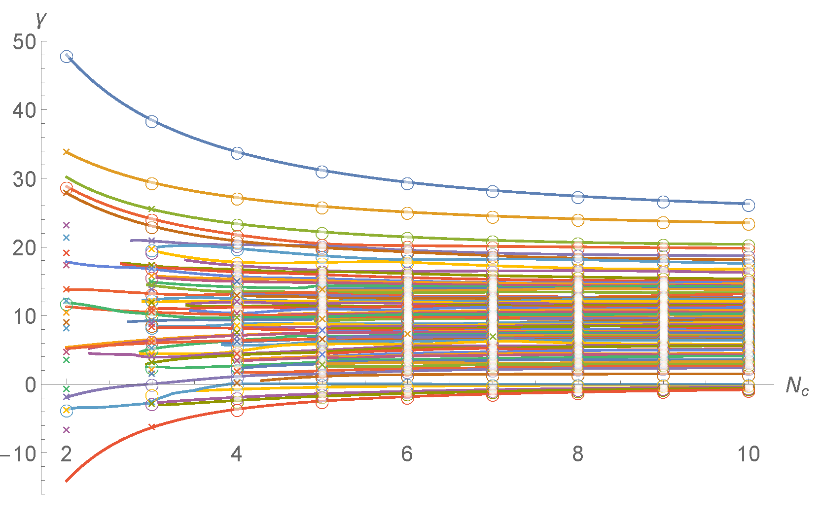
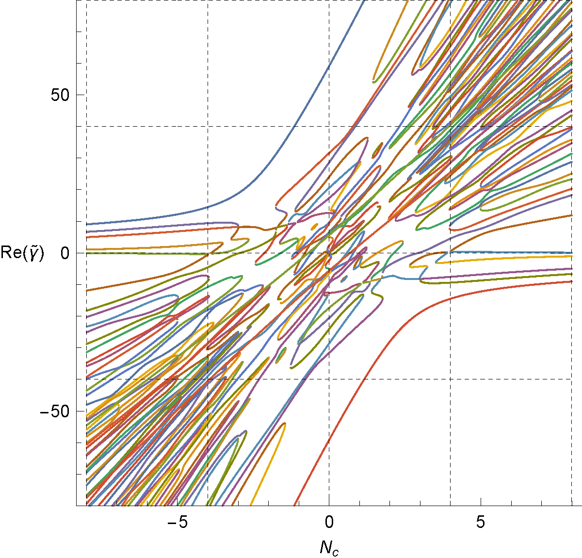
Also, there is a pair of exceptional operators at , which take the form
| (B.12) |
and their one-lop dimensions are exactly given by
| (B.13) |
There are five large zero modes. The submixing matrix for general is given by
| (B.14) | ||||
| (B.15) |
These matrix elements are defined on the basis272727The off-diagonal elements of depend on the normalization of . Here we use the convention: .
| (B.16) |
where is the following combination of two quadruple traces,
| (B.17) | |||
By diagonalizing the submixing matrix at , one finds
| (B.18) |
where are for -trace operators. The operator corresponding to is not protected, and receives corrections at with a positive sign.
Degeneracy of non-zero modes.
There are six degenerate positive eigenvalues at , namely . The eigenvalues receive finite corrections at the order , and the large expansion of these modes can submix with the operators having different number of traces. They make a contrast to the properties of the large zero modes . For example, the eigenstates corresponding to the eigenvalue 6 take the form
| (B.19) |
where is a multi-trace operator with length .
B.2.4
There are 469 singlets at length . The mixing matrix and operator basis for general are shown in the attached files AncillaryNegative.nb and AncillaryL10Data.txt. The spectrum is shown in Figure 10.282828We have not checked potential level-crossing with exceptional eigenvalues due to the complexity. To highlight the structure of the spectrum lying in the middle, we plot the eigenvalue density in Figure 11.
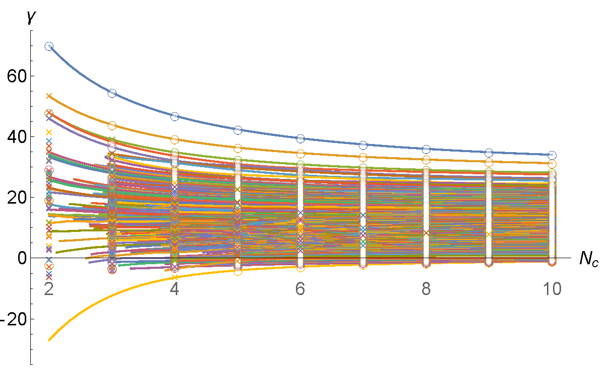
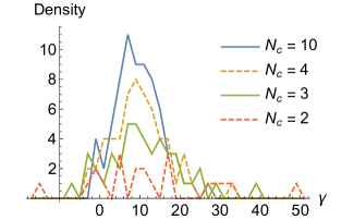
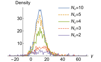
There are 11 large zero modes, as shown in . There are no finite - zero modes. At , the submixing matrix has two zero modes corresponding to combinations of quadruple- and quintuple-trace operators. The one-loop dimensions of two operators are and positive. The submixing matrix at is given by
| (B.20) |
which is block-diagonal. These matrix elements are defined on the basis
| (B.21) |
where means linear combinations of the large zero modes with -traces, and explicitly given in . The eigenvalues of the submixing matrix is
| (B.22) |
Only numerical values are shown in because their precise forms are quite complicated. For example, the eigenvalue for the double-trace mode is
| (B.23) |
B.2.5
There are 4477 singlets at length . We have not made a detailed analysis of the spectrum due to a huge amount of computation involved. There are 34 large zero modes,
| (B.24) |
in the notation of .
B.3 Spectrum at general
We consider the spectrum of submixing matrix for singlets at general , which will highlight the special properties of SYM from the non-planar spectrum of other gauge theories. The value corresponds to SYM.
Let us outline two properties of the spectrum of the submixing Hamiltonian at general . First, decrease as increases,
| (B.25) |
It shows that the leading corrections to the large zero modes can be positive when as shown in Figure 12.
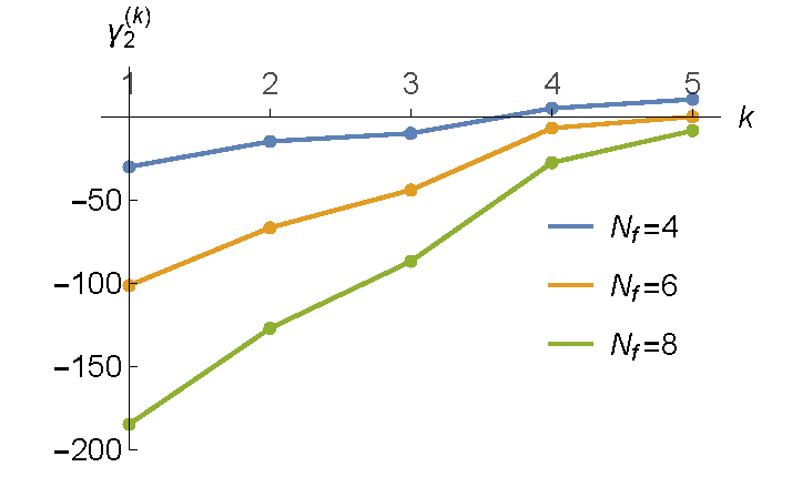
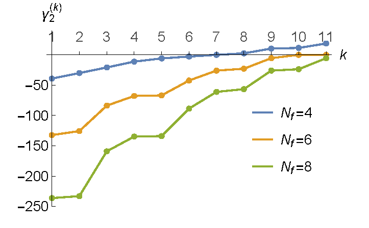
Second, all eigenvalues of the submixing matrix scale as in the large limit,292929The limit does not commute with , so we consider .
| (B.26) |
with some coefficient . This scaling behavior can be seen from the submixing matrix at given in , , . Moreover, the large approximation is numerically not bad. Figure 13 shows that the rescaled eigenvalues do not deviate a lot from the data.
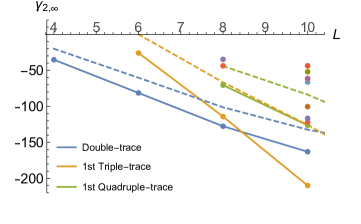
Appendix C Correlation functions at large
We explain the details of the computation in Section 3.
C.1 A proof of at large
In this subsection, we will show that the first term of , , is always non-positive by making use of the limit .303030 In general is given by a linear combination of the large zero modes as . Because off-diagonal expectation values () cannot have the leading power with respect to both and , we may consider only diagonal expectation values .
Since , we can consider . For convenience, we rename each term of the one-loop dilatation operator by
| (C.1) |
where
| (C.2) |
and
| (C.3) |
Suppose that acts on
| (C.4) |
where one derivative in acts on one of the ’s in the first trace and the other derivative acts on one of the ’s in the second trace. We denote the remaining traces of by , i.e. .
We can find that the leading behavior of in the correlator is . The leading power arises if the following two conditions are satisfied: (a) the two derivatives in act on two ’s, giving and replacing them with ’s, (b) when a (or ) is Wick-contracted with a , the other (or ) is also Wick-contracted with the other , giving . Because the factor cannot arise from the action of , only the action of may be considered in what follows. At large , the traceless part of does not give the leading contribution.
When the conditions (a) and (b) are satisfied, the correlator can be reduced as
| (C.5) |
At the last step, we performed Wick-contractions in and simplified the flavor indices using the ’s. In the reduced correlator, all flavor indices are contracted. Then, the dilatation operator makes a single trace from , removing two ’s and putting two ’s. More precisely, put two ’s away from each other while put them next to each other, as shown in (A.11) and (A.13). When two ’s are adjacent in the reduced correlator, we have a smaller symmetry factor than the non-adjacent case. This difference in symmetry factor is the reason the correlator is non-positive.
The following is an example. Consider a reduced correlator
| (C.6) |
This is a case of and . It has the following two contributions:313131 The symmetry factor in (C.7) can be explained as follows. When in the first trace is Wick-contracted with the first , in the second trace must be Wick-contracted with the second . To keep the planarity, we should Wick-contract the first with the first , and the second with the second , and so on. We say this that are Wick-contracted with . Likewise can be Wick-contracted with for any while keeping the planarity. In this way, we get the factor . The factor comes from exchanging two single traces.
| (C.7) | |||||
and323232The symmetry factor
(C.8) comes from
the Wick-contractions between
and only.
It can be more manifest if we write the correlator as
.
| (C.8) | |||||
where we have kept only the leading term with respect to and . Because , the correlator (C.6) is negative.
C.2 and dependence of
In this subsection, we will consider the expansion to study the -dependence of for the operators presented in Section 3.3. General properties of will be first discussed, and then concrete examples are shown.
Recall the expression of :
| (C.9) |
As we discussed in the last subsection, the first term behaves as , and as we will see below the second term has a more dominant behavior .
The relation between and is given by the equation 333333 in (3.21) is not important at the leading order of the expansion in , so we can use . obtained in (3.21), which can rewrite the second term as
| (C.10) |
Focusing only on the leading of the expansion, we find that can be expanded as
| (C.11) |
where is multi-traces without the factor . is a multi-trace that does not contain two adjacent matrices with the flavor indices contracted, and is a multi-trace that does contain such matrices. They appeared in the image of and respectively; see the second lines of and as well as (C.15) for the double-trace operator. The comes from the action of .
The planar dilatation operator has the form , where , and are the identity, the transposition and the contraction acting on nearest neighbor matrices. Only the contraction can bring a factor of . In order to determine the form of , we need to solve . Since and , the solution is roughly written as
| (C.12) |
where and are -independent coefficients. Substituting these equations into the form of , we have
| (C.13) |
where the ratio of the two-point functions is independent of . The behavior of is consistent with (B.26). It is emphasized that in (C.11) does not matter for the evaluation of at the leading order.
Our next goal is to estimate the -dependence of the correlators. The double-trace operator and -trace operators are studied below.
Consider the singlet double trace operator (3.36). We will use the property of the symmetric representation , and
| (C.14) | |||||
where , and the factor comes from the normalization of the projector.
Acting with on , we have
| (C.15) | |||||
The multi-traces and belong to and respectively. Note that the flavor indices are in the irreducible representation , where represents the rank- symmetric traceless representation.
We have to solve the equation . Suppose that the solution is given by
| (C.16) |
where is an -independent positive constant that may depend on . Other terms are denoted by , expecting that they do not change the -dependence at the leading order of the expansion. We will leave it as a future problem to determine . We then have
| (C.17) |
The normalization was computed in (3.38), which is evaluated at large as 343434 The dimension of the rank- traceless symmetric representation of is (C.18) where we have approximated using Stirling’s formula for . The result (C.19) can also be obtained by considering only Wick-contractions that satisfy the condition (b) in the last subsection.
| (C.19) |
and we also have
| (C.20) |
to obtain
| (C.21) |
Therefore the double-trace operator scale as .
The next study is about -trace operators such as and . These multi-traces have the same color structure, but the flavor indices are contracted differently. As we mentioned in Section 3.3, such multi-traces can be classified by the partitions of , and we write them by , where expresses a partition of .
In general, a submixing eigenstate is a linear combination of ’s. This situation simplifies at large , where the two-point functions are orthogonal and the submixing Hamiltonian acts diagonally on . Then is expressed by
| (C.22) |
For ,353535 Introduced the notation . we obtain
| (C.23) |
The two-point functions can be computed
| (C.24) |
to obtain
| (C.25) |
where is determined by the equation
| (C.26) |
The two expressions (C.21) and (C.25) agree at as expected. The equation shows that the -trace scale like as a function of .
Consider more general -trace operators , where , and we assume for simplicity. We then have
| (C.27) | |||||
and
| (C.28) |
where . Substituting these two-point functions into the expression of , we will obtain
| (C.29) | |||||
where is another positive constant in , which is determined by the equation . We leave it for a future problem to determine the precise dependence.
Appendix D Relation to Mandelstam Variables
We pursue the coincidence between the number of singlet large zero-modes in Table 1 in Section 2.3 and the number of the completely symmetric polynomial of Mandelstam variables under certain conditions in Table 2 of [60]. This fact allows us to construct an explicit basis for the latter.
We defined as the number of singlet large zero modes with length . These zero-modes can be written explicitly in terms of the traceless symmetric single-trace operators as
| (D.1) |
corresponding to .
Another series of positive integers is computed in [60], which is the number of the completely symmetric polynomial of Mandelstam variables of degree , subject to massless momentum conservation, for a sufficiently large number of particles . If we denote this series by , they are given by . The Mandelstam variables are defined by
| (D.2) |
and they satisfy
| (D.3) |
A basis of the completely symmetric polynomials of can be given as
| (D.4) |
where we sum over the permutation group of -th order . The constraints must be imposed after the summation.
The relation between and can be explained graphically. Note that we neglect dimensionality constraints; namely the finite constraints in and the Gram determinant constraints in .363636The latter comes from the linear relations among when is greater than the spacetime dimensions.
We begin by the singlet large zero modes. Since is symmetric traceless, a flavor index of should be paired with the flavor index of another . Since is symmetric, the position of the flavor index inside is irrelevant. When we contract indices of and , we draw lines in between as
| (D.5) |
Similarly, the zero modes with length six are expressed as
| (D.6) |
and with length eight as,
| (D.7) |
Let us turn to the completely symmetric polynomials of Mandelstam variables Given a graph representing the large zero modes, we label each “single-trace” by . Then for each line connecting the -th and -th trace, we associate Mandelstam variable , as
| (D.8) |
which gives the first line of . Similarly, a basis of the completely symmetric polynomials of degree three is expressed as
| (D.9) |
One can check that the length eight graphs reproduce the polynomials of degree four in .
This pattern continues. At we have . The correspondence can be seen from
| (D.10) |
and
| (D.11) |
where means the sum over the permutations . Note that the all terms add up with the same sign.
It is not obvious to prove the linear independence when the massless momentum conservations are imposed. For example, there are three candidates of the symmetric polynomials at degree two,
| (D.12) |
It turns out that and when the constraints are imposed. This can be shown, for example, by applying the condition repeatedly, until there are no indices which appear only once. We checked that the polynomials written in our “graphical basis” are linearly independent up to . It also follows that our basis is complete thanks to .
We also emphasize that it is non-trivial to construct an explicit basis of the completely symmetric polynomials of . A candidate is given by taking multi-traces of the matrix of Mandelstam variables,
| (D.13) |
These polynomials are manifestly invariant under permutations, but highly redundant even before imposing the massless momentum conservation. It is not clear how to take a linearly independent set.
When we turn on masses, the momentum conservation becomes
| (D.14) |
and the number of independent completely symmetric polynomials increases. For example, three degree-two polynomials in are no longer proportional. The corresponding generalization in SYM will be to consider gauge group instead of .
It is interesting to see how the above relation can be proven for general , and whether the correspondence can be extended to massive cases.
Appendix E Polynomial notation for multi-traces
A new concise notation for multi-trace operators is invented to reduce the computational workload significantly in Mathematica. We call it polynomial notation, which can be used to describe any gauge invariant operators of SYM.
We associate a polynomial to each multi-trace operator. The basic idea is to describe the position inside a trace at which a given SYM field appears, rather than to describe which SYM field appears at a given position inside a trace.
First, consider single-trace operators. If a field stands at the -th position inside the trace, we write , then sum over all fields as
| (E.1) |
where means that this polynomial is defined modulo cyclic permutation of a trace,
| (E.2) |
For later purposes, we rewrite this equation as
| (E.3) |
where is the shift operator defined by
| (E.4) |
Next, we generalize this notation to the operators with flavor indices contracted, like for the singlets and for the singlets, where . If is at the -th position and is at the -th position, we write
| (E.5) |
The singlets can be expressed by imposing the relation .373737We keep to avoid confusion between and . This polynomial notation is significantly simpler than the usual one because no flavor subscripts are used anymore. To see this, consider the following singlet operator of length four,
| (E.6) |
On the left-hand side, we wrote two identical operators generated by the permutation of flavor indices with . As increases, the order of the permutation group grows factorially. It becomes quite cumbersome to keep removing redundant elements generated by . In this sense, the polynomial notation is factorially simpler to describe single-trace operators than the conventional notation.383838The polynomial notation becomes less efficient if we consider multi-trace operators, particularly those containing single-traces of the same length. The computation using the polynomial notation is faster overall.
Second, consider multi-trace operators. If a field stands at the -th position inside the -th trace, we write , then sum over all fields as
| (E.7) |
where means that we contract at the -th position in the -th trace and at the -th position in the -th trace. We impose the cyclicity condition as
| (E.8) |
where is the shift operator for the -th trace.
The polynomial notation is related to a graphical representation of multi-trace operators as follows:
| (E.9) | |||
| (E.10) |
where the black dashed lines represent the color traces, and the blue solid lines represent flavor contractions. The middle equality in the last line comes from the cyclic symmetry of the trace. In short, the polynomial notation describes the configuration of the blue lines. Note also that a similar graphical method was useful in finding the relation to Mandelstam variables in Appendix D.
We generated all singlet multi-trace operators up to using Mathematica, and implemented the action of the non-planar dilatation operator in the polynomial notation. The details are given in the attached file.
References
- [1] G. ’t Hooft, “A Planar Diagram Theory for Strong Interactions,” Nucl. Phys. B 72 (1974) 461.
- [2] J. M. Maldacena, “The Large limit of superconformal field theories and supergravity,” Int. J. Theor. Phys. 38 (1999) 1113 [Adv. Theor. Math. Phys. 2 (1998) 231] [hep-th/9711200].
- [3] N. Beisert et al., “Review of AdS/CFT Integrability: An Overview,” Lett. Math. Phys. 99 (2012) 3 [arXiv:1012.3982 [hep-th]].
- [4] L. Cornalba, M. S. Costa, J. Penedones and R. Schiappa, “Eikonal Approximation in AdS/CFT: From Shock Waves to Four-Point Functions,” JHEP 0708 (2007) 019 [hep-th/0611122].
- [5] L. Cornalba, M. S. Costa, J. Penedones and R. Schiappa, “Eikonal Approximation in AdS/CFT: Conformal Partial Waves and Finite Four-Point Functions,” Nucl. Phys. B 767 (2007) 327 [hep-th/0611123].
- [6] L. Cornalba, M. S. Costa and J. Penedones, “Eikonal approximation in AdS/CFT: Resumming the gravitational loop expansion,” JHEP 0709 (2007) 037 [arXiv:0707.0120 [hep-th]].
- [7] X. O. Camanho, J. D. Edelstein, J. Maldacena and A. Zhiboedov, “Causality Constraints on Corrections to the Graviton Three-Point Coupling,” arXiv:1407.5597 [hep-th].
- [8] Z. Bajnok, N. Drukker, Á. Hegedüs, R. I. Nepomechie, L. Palla, C. Sieg and R. Suzuki, “The spectrum of tachyons in AdS/CFT,” JHEP 1403 (2014) 055 [arXiv:1312.3900 [hep-th]].
- [9] Á. Hegedűs, “Extensive numerical study of a D-brane, anti-D-brane system in /,” JHEP 1504 (2015) 107 [arXiv:1501.07412 [hep-th]].
- [10] S. Corley, A. Jevicki and S. Ramgoolam, “Exact correlators of giant gravitons from dual Sym theory,” Adv. Theor. Math. Phys. 5 (2002) 809 [hep-th/0111222].
- [11] V. Balasubramanian, D. Berenstein, B. Feng and M. x. Huang, “D-branes in Yang-Mills theory and emergent gauge symmetry,” JHEP 0503 (2005) 006 [hep-th/0411205].
- [12] R. Bhattacharyya, S. Collins and R. d. M. Koch, “Exact Multi-Matrix Correlators,” JHEP 0803 (2008) 044 [arXiv:0801.2061 [hep-th]].
- [13] Y. Kimura and S. Ramgoolam, “Branes, anti-branes and brauer algebras in gauge-gravity duality,” JHEP 0711 (2007) 078 [arXiv:0709.2158 [hep-th]].
- [14] Y. Kimura, “Non-holomorphic multi-matrix gauge invariant operators based on Brauer algebra,” JHEP 0912 (2009) 044 [arXiv:0910.2170 [hep-th]].
- [15] Y. Kimura, “Correlation functions and representation bases in free Super Yang-Mills,” Nucl. Phys. B 865 (2012) 568 [arXiv:1206.4844 [hep-th]].
- [16] T. W. Brown, P. J. Heslop and S. Ramgoolam, “Diagonal multi-matrix correlators and BPS operators in Sym,” JHEP 0802 (2008) 030 [arXiv:0711.0176 [hep-th]].
- [17] T. W. Brown, P. J. Heslop and S. Ramgoolam, “Diagonal free field matrix correlators, global symmetries and giant gravitons,” JHEP 0904 (2009) 089 [arXiv:0806.1911 [hep-th]].
- [18] R. de Mello Koch, J. Smolic and M. Smolic, “Giant Gravitons - with Strings Attached (II),” JHEP 0709 (2007) 049 [hep-th/0701067].
- [19] T. W. Brown, “Permutations and the Loop,” JHEP 0806 (2008) 008 [arXiv:0801.2094 [hep-th]].
- [20] R. d. M. Koch, G. Mashile and N. Park, “Emergent Threebrane Lattices,” Phys. Rev. D 81 (2010) 106009 [arXiv:1004.1108 [hep-th]].
- [21] V. De Comarmond, R. de Mello Koch and K. Jefferies, “Surprisingly Simple Spectra,” JHEP 1102 (2011) 006 [arXiv:1012.3884 [hep-th]].
- [22] W. Carlson, R. d. M. Koch and H. Lin, “Nonplanar Integrability,” JHEP 1103 (2011) 105 [arXiv:1101.5404 [hep-th]].
- [23] R. d. M. Koch, M. Dessein, D. Giataganas and C. Mathwin, “Giant Graviton Oscillators,” JHEP 1110 (2011) 009 [arXiv:1108.2761 [hep-th]].
- [24] R. de Mello Koch, P. Diaz and H. Soltanpanahi, “Non-planar Anomalous Dimensions in the sl(2) Sector,” Phys. Lett. B 713 (2012) 509 [arXiv:1111.6385 [hep-th]].
- [25] R. de Mello Koch and S. Ramgoolam, “A double coset ansatz for integrability in AdS/CFT,” JHEP 1206 (2012) 083 [arXiv:1204.2153 [hep-th]].
- [26] R. de Mello Koch, S. Graham and I. Messamah, “Higher Loop Nonplanar Anomalous Dimensions from Symmetry,” JHEP 1402 (2014) 125 [arXiv:1312.6227 [hep-th]].
- [27] H. Lin, “Relation between large dimension operators and oscillator algebra of Young diagrams,” Int. J. Geom. Meth. Mod. Phys. 12 (2015) 04, 1550047 [arXiv:1407.7815 [hep-th]].
- [28] N. Beisert, C. Kristjansen, J. Plefka, G. W. Semenoff and M. Staudacher, “ BMN correlators and operator mixing in superYang-Mills theory,” Nucl. Phys. B 650 (2003) 125 [hep-th/0208178].
- [29] N. Beisert, C. Kristjansen, J. Plefka and M. Staudacher, “ BMN gauge theory as a quantum mechanical system,” Phys. Lett. B 558 (2003) 229 [hep-th/0212269].
- [30] C. Kristjansen, “Review of AdS/CFT Integrability, Chapter IV.1: Aspects of Non-Planarity,” Lett. Math. Phys. 99 (2012) 349 [arXiv:1012.3997 [hep-th]].
- [31] V. N. Velizhanin, “The Non-planar contribution to the four-loop universal anomalous dimension in Supersymmetric Yang-Mills theory,” JETP Lett. 89 (2009) 593 [arXiv:0902.4646 [hep-th]].
- [32] J. A. Minahan and K. Zarembo, “The Bethe ansatz for superYang-Mills,” JHEP 0303 (2003) 013 [hep-th/0212208].
- [33] E. D’Hoker, S. D. Mathur, A. Matusis and L. Rastelli, “The Operator product expansion of Sym and the 4 point functions of supergravity,” Nucl. Phys. B 589 (2000) 38 [hep-th/9911222].
- [34] G. Arutyunov, S. Frolov and A. C. Petkou, “Operator product expansion of the lowest weight CPOs in SYM(4) at strong coupling,” Nucl. Phys. B 586 (2000) 547 [Nucl. Phys. B 609 (2001) 539] [hep-th/0005182].
- [35] L. I. Uruchurtu, “AdS/CFT for Four-Point Amplitudes involving Gravitino Exchange,” JHEP 0709 (2007) 086 [arXiv:0707.0424 [hep-th]].
- [36] J. A. Minahan and R. Pereira, “Three-point correlators from string amplitudes: Mixing and Regge spins,” JHEP 1504 (2015) 134 [arXiv:1410.4746 [hep-th]].
- [37] V. Gonçalves, “Four point function of stress-tensor multiplet at strong coupling,” JHEP 1504 (2015) 150 [arXiv:1411.1675 [hep-th]].
- [38] M. Bianchi, S. Kovacs, G. Rossi and Y. S. Stanev, “On the logarithmic behavior in Sym theory,” JHEP 9908 (1999) 020 [hep-th/9906188].
- [39] G. Arutyunov, F. A. Dolan, H. Osborn and E. Sokatchev, “Correlation functions and massive Kaluza-Klein modes in the AdS / CFT correspondence,” Nucl. Phys. B 665 (2003) 273 [hep-th/0212116].
- [40] G. Arutyunov, S. Penati, A. C. Petkou, A. Santambrogio and E. Sokatchev, “Nonprotected operators in Sym and multiparticle states of Sugra,” Nucl. Phys. B 643 (2002) 49 [hep-th/0206020].
- [41] G. Arutyunov, S. Penati, A. Santambrogio and E. Sokatchev, “Four point correlators of BPS operators in Sym at order ,” Nucl. Phys. B 670 (2003) 103 [hep-th/0305060].
- [42] F. A. Dolan and H. Osborn, “Superconformal symmetry, correlation functions and the operator product expansion,” Nucl. Phys. B 629 (2002) 3 [hep-th/0112251].
- [43] M. Bianchi, F. A. Dolan, P. J. Heslop and H. Osborn, “ superconformal characters and partition functions,” Nucl. Phys. B 767 (2007) 163 [hep-th/0609179].
- [44] L. F. Alday and A. Bissi, “Generalized bootstrap equations for SCFT,” JHEP 1502 (2015) 101 [arXiv:1404.5864 [hep-th]].
- [45] L. F. Alday, A. Bissi and T. Lukowski, “Lessons from crossing symmetry at large N,” JHEP 1506 (2015) 074 [arXiv:1410.4717 [hep-th]].
- [46] A. Kaviraj, K. Sen and A. Sinha, “Analytic bootstrap at large spin,” arXiv:1502.01437 [hep-th].
- [47] V. Balasubramanian, M. Berkooz, A. Naqvi and M. J. Strassler, “Giant gravitons in conformal field theory,” JHEP 0204 (2002) 034 [hep-th/0107119].
- [48] D. Berenstein and S. E. Vazquez, “Integrable open spin chains from giant gravitons,” JHEP 0506 (2005) 059 [hep-th/0501078].
- [49] D. M. Hofman and J. M. Maldacena, “Reflecting magnons,” JHEP 0711 (2007) 063 [arXiv:0708.2272 [hep-th]].
- [50] J. von Neumann and E. Wigner,“Über das Verhalten von Eigenwerten bei adiabatischen Prozessen," Physikalische Zeitschrift 30 (1929) 467.
- [51] D. J. Gross, A. Mikhailov and R. Roiban, “A Calculation of the plane wave string Hamiltonian from superYang-Mills theory,” JHEP 0305 (2003) 025 [hep-th/0208231].
- [52] L. Andrianopoli, S. Ferrara, E. Sokatchev and B. Zupnik, “Shortening of primary operators in extended SCFT(4) and harmonic superspace analyticity,” Adv. Theor. Math. Phys. 4 (2000) 1149 [hep-th/9912007].
- [53] E. D’Hoker and D. Z. Freedman, “Supersymmetric gauge theories and the AdS / CFT correspondence,” hep-th/0201253.
- [54] A. V. Ryzhov, “Quarter BPS operators in Sym,” JHEP 0111 (2001) 046 [hep-th/0109064].
- [55] E. D’Hoker, P. Heslop, P. Howe and A. V. Ryzhov, “Systematics of quarter BPS operators in Sym,” JHEP 0304 (2003) 038 [hep-th/0301104].
- [56] T. W. Brown, “Cut-and-join operators and super Yang-Mills,” JHEP 1005 (2010) 058 [arXiv:1002.2099 [hep-th]].
- [57] Y. Kimura, “Quarter BPS classified by Brauer algebra,” JHEP 1005 (2010) 103 [arXiv:1002.2424 [hep-th]].
- [58] J. Pasukonis and S. Ramgoolam, “From counting to construction of BPS states in Sym,” JHEP 1102 (2011) 078 [arXiv:1010.1683 [hep-th]].
-
[59]
OEIS Foundation Inc. (2011), the On-Line Encyclopedia of Integer Sequences,
https://oeis.org/A226919 - [60] R. H. Boels, “On the field theory expansion of superstring five point amplitudes,” Nucl. Phys. B 876 (2013) 215 [arXiv:1304.7918 [hep-th]].
- [61] N. Beisert, C. Kristjansen and M. Staudacher, “The Dilatation operator of conformal superYang-Mills theory,” Nucl. Phys. B 664 (2003) 131 [hep-th/0303060].
- [62] M. Bianchi, G. Rossi and Y. S. Stanev, “Surprises from the resolution of operator mixing in Sym,” Nucl. Phys. B 685 (2004) 65 [hep-th/0312228].
- [63] Y. Kimura and S. Ramgoolam, “Enhanced symmetries of gauge theory and resolving the spectrum of local operators,” Phys. Rev. D 78 (2008) 126003 [arXiv:0807.3696 [hep-th]].
- [64] N. R. Constable, D. Z. Freedman, M. Headrick and S. Minwalla, “Operator mixing and the BMN correspondence,” JHEP 0210 (2002) 068 [hep-th/0209002].
- [65] G. Grignani, M. Orselli, B. Ramadanovic, G. W. Semenoff and D. Young, “Divergence cancellation and loop corrections in string field theory on a plane wave background,” JHEP 0512 (2005) 017 [hep-th/0508126].
- [66] S. Corley and S. Ramgoolam, “Finite factorization equations and sum rules for BPS correlators in Sym theory,” Nucl. Phys. B 641 (2002) 131 [hep-th/0205221].
- [67] F. Gonzalez-Rey, I. Y. Park and K. Schalm, “A Note on four point functions of conformal operators in superYang-Mills,” Phys. Lett. B 448 (1999) 37 [hep-th/9811155].
- [68] B. Eden, P. S. Howe, C. Schubert, E. Sokatchev and P. C. West, “Four point functions in supersymmetric Yang-Mills theory at two loops,” Nucl. Phys. B 557 (1999) 355 [hep-th/9811172].
- [69] F. A. Dolan and H. Osborn, “Conformal partial wave expansions for chiral four point functions,” Annals Phys. 321 (2006) 581 [hep-th/0412335].
- [70] N. Drukker and J. Plefka, “The Structure of n-point functions of chiral primary operators in super Yang-Mills at one-loop,” JHEP 0904 (2009) 001 [arXiv:0812.3341 [hep-th]].
- [71] G. Arutyunov, M. de Leeuw and S. J. van Tongeren, “Twisting the Mirror TBA,” JHEP 1102 (2011) 025 [arXiv:1009.4118 [hep-th]].
- [72] J. Fokken, C. Sieg and M. Wilhelm, “The complete one-loop dilatation operator of planar real -deformed Sym theory,” JHEP 1407 (2014) 150 [arXiv:1312.2959 [hep-th]].
- [73] C. Vafa, “Non-Unitary Holography,” arXiv:1409.1603 [hep-th].
- [74] T. Okuda and T. Takayanagi, “Ghost D-branes,” JHEP 0603 (2006) 062 [hep-th/0601024].
- [75] P. Caputa, C. Kristjansen and K. Zoubos, “On the spectral problem of Sym with orthogonal or symplectic gauge group,” JHEP 1010 (2010) 082 [arXiv:1005.2611 [hep-th]].
- [76] P. Caputa, R. d. M. Koch and P. Diaz, “Operators, Correlators and Free Fermions for and Sp(N),” JHEP 1306 (2013) 018 [arXiv:1303.7252 [hep-th]].
- [77] G. Kemp, “Restricted Schurs and correlators for and Sp(N),” JHEP 1408 (2014) 137 [arXiv:1406.3854 [hep-th]].
- [78] Y. Makeenko, “Large gauge theories,” NATO Sci. Ser. C 556 (2000) 285 [hep-th/0001047].
- [79] R. Ishizeki and M. Kruczenski, “Single spike solutions for strings on and S**3,” Phys. Rev. D 76 (2007) 126006 [arXiv:0705.2429 [hep-th]].
- [80] H. Hayashi, K. Okamura, R. Suzuki and B. Vicedo, “Large Winding Sector of AdS/CFT,” JHEP 0711 (2007) 033 [arXiv:0709.4033 [hep-th]].
- [81] N. Berkovits and J. Maldacena, “Fermionic T-Duality, Dual Superconformal Symmetry, and the Amplitude/Wilson Loop Connection,” JHEP 0809 (2008) 062 [arXiv:0807.3196 [hep-th]].
- [82] M. Kruczenski and A. A. Tseytlin, “Wilson loops T-dual to Short Strings,” Nucl. Phys. B 875 (2013) 213 [arXiv:1212.4886 [hep-th]].
- [83] M. C. Abbott and I. V. Aniceto, “Vibrating giant spikes and the large-winding sector,” JHEP 0806 (2008) 088 [arXiv:0803.4222 [hep-th]].
- [84] E. Witten, “Baryons and branes in anti-de Sitter space,” JHEP 9807 (1998) 006 [hep-th/9805112].
- [85] G. Mack, “D-independent representation of Conformal Field Theories in D dimensions via transformation to auxiliary Dual Resonance Models. Scalar amplitudes,” arXiv:0907.2407 [hep-th].
- [86] G. Mack, “D-dimensional Conformal Field Theories with anomalous dimensions as Dual Resonance Models,” Bulg. J. Phys. 36 (2009) 214 [arXiv:0909.1024 [hep-th]].
- [87] J. Penedones, “Writing CFT correlation functions as AdS scattering amplitudes,” JHEP 1103 (2011) 025 [arXiv:1011.1485 [hep-th]].
- [88] N. Y. Reshetikhin, “A Method of Functional Equations in the Theory of Exactly Solvable Quantum Systems,” Lett. Math. Phys. 7 (1983) 205.
- [89] N. Y. Reshetikhin, “Integrable Models of Quantum One-dimensional Magnets with O(N) and Sp(2k) Symmetry,” Theor. Math. Phys. 63 (1985) 555 [Teor. Mat. Fiz. 63 (1985) 347].
- [90] J. M. Maldacena and A. Strominger, “Ad black holes and a stringy exclusion principle,” JHEP 9812 (1998) 005 [hep-th/9804085].
- [91] M. Bianchi, B. Eden, G. Rossi and Y. S. Stanev, “On operator mixing in Sym,” Nucl. Phys. B 646 (2002) 69 [hep-th/0205321].
- [92] V. A. Fateev, A. V. Litvinov, A. Neveu and E. Onofri, “Differential equation for four-point correlation function in Liouville field theory and elliptic four-point conformal blocks,” J. Phys. A 42 (2009) 304011 [arXiv:0902.1331 [hep-th]].
- [93] R. Poghossian, “Recursion relations in CFT and Sym theory,” JHEP 0912 (2009) 038 [arXiv:0909.3412 [hep-th]].
- [94] L. Hadasz, Z. Jaskolski and P. Suchanek, “Recursive representation of the torus 1-point conformal block,” JHEP 1001 (2010) 063 [arXiv:0911.2353 [hep-th]].
- [95] L. F. Alday and A. Bissi, “Modular interpolating functions for Sym,” JHEP 1407 (2014) 007 [arXiv:1311.3215 [hep-th]].