Applying a formula for generator redispatch to damp interarea oscillations using synchrophasors

Abstract

If an interarea oscillatory mode has insufficient damping, generator redispatch can be used to improve its damping. We explain and apply a new analytic formula for the modal sensitivity to rank the best pairs of generators to redispatch. The formula requires some dynamic power system data and we show how to obtain that data from synchrophasor measurements. The application of the formula to damp interarea modes is explained and illustrated with interarea modes of the New England 10-generator power system.

I Introduction

Power transmission systems have multiple electromechanical oscillatory modes in which power system areas can swing against each other. In large grids, these interarea oscillations typically have low frequency in the range 0.1 to 1.0 Hz, and can appear for large or unusual power transfers. Poorly damped or negatively damped oscillations can become more frequent as power systems experience greater variability of loading conditions and can lead to equipment damage, malfunction or blackouts. Practical rules for power system security often require sufficient damping of oscillatory modes [1, 2], such as damping ratio of at least 5%, and power transfers on tie lines are sometimes limited by oscillations [1, 3, 4, 5].

There are several approaches to maintaining sufficient damping of oscillatory modes, including limiting power transfers [6], installing closed loop controls [1], and the approach of this paper, which is to take operator actions such as redispatching generation [6, 7, 8]. It is now feasible to monitor modal damping and frequency online from synchrophasors (also known as PMUs) [9, 10]. Suppose that a mode with insufficient damping ratio is detected. Then what actions should be taken to restore the mode damping?

This paper calculates the best generator pairs to redispatch to maintain the mode damping by combining synchrophasor and state estimator measurements with a new analytic formula for the sensitivity of the mode eigenvalue with respect to generator redispatch. This formula, previously thought to be unattainable, is derived with a combination of new and old methods in [11]. The length of the derivation (more than 8 pages) precludes its presentation here. In this paper we state, explain, and demonstrate the application of the new formula and show how the terms of the formula could be obtained from power system measurements. In particular, we propose using synchrophasors to measure the terms of the formula that depend on dynamics and using the state estimator to measure the terms of the formula that depend on statics. In applying a first order sensitivity formula, we assume that the power system ambient or transient behavior is dominated by the linearized dynamics associated with an asymptotically stable operating equilibrium.

Changes in generator dispatch change the oscillation damping by exploiting nonlinearity of the power system: changing the dispatch changes the operating equilibrium and hence the linearization of the power system about that equilibrium that determines the oscillatory modes and their damping. This open loop approach that applies an operator action after too little damping is detected can be contrasted with an approach that designs closed loop controls to damp the oscillations preventively. The closed loop control design chooses control gains that appear explicitly in the power system Jacobian, whereas generator redispatch changes the Jacobian indirectly by changing the operating point at which the Jacobian is evaluated.

We now review previous works using generator redispatch to damp oscillations; these have considered heuristics, brute force computations, and formulas that are difficult to implement from measurements. These approaches have established that generator redispatch can damp oscillatory modes.

Fischer and Erlich pioneered heuristics for the redispatch in terms of the mode shapes for some simple grid structures and for the European grid [8, 12]. Their heuristics seem promising for insights, elaborations and validation, especially since there has also been progress in determining the mode shape from measurements [13, 14, 15, 16].

There are also previous approaches that require a dynamic grid model. The effective generator redispatches can be determined by repetitive computation of eigenvalues of a dynamic power grid model to give numerical sensitivities [5, 6, 17, 18]. Also, there are exact computations of the sensitivity of the damping from a dynamic power grid model [7, 19, 20, 21] that are based on the eigenvalue sensitivity formula

$$\frac{\partial\lambda}{\partial p}=\frac{wJ_{p}v}{wv},$$ (1)

where $w$ and $v$ are left and right eigenvectors associated with the eigenvalue $\lambda$ and $J_{p}$ is the derivative of the Jacobian with respect to the amount of generator redispatch $p$. The calculation of $J_{p}$ involves the Hessian and the sensitivity of the operating point to $p$. However, requiring a large scale power system dynamic model poses difficulties. It is challenging to obtain validated models of generator dynamics over a wide area and particularly difficult to determine dynamic load models that would be applicable online when poor modal damping arises.

We think that a good way to solve the difficulties with online large scale power system dynamic models is to combine models with synchrophasor measurements to get actionable information about mode damping. In particular, the dynamic information about the power system can be estimated from synchrophasors. However, formula (1) is not suitable for this purpose since it is not feasible to estimate from measurements the left eigenvector $w$ in (1) (or derivatives of eigenvectors in other versions of (1)). This was a primary motivation for developing our new formula in [11]. In particular, the formula shows that the first order effect of a generator redispatch largely depends on the mode shape (the right eigenvector) and power flow quantities that can be measured online. The assumed equivalent generator dynamics only appears as a factor common to all redispatches. Given a lightly damped interarea mode of a system, the method can rank all the possible generators pairs. The rank is based on the size of the change of the damping ratio of the interarea mode.

The main objective of ranking the generator pairs is to provide advice to the operator of several effective generator redispatches to damp the oscillations from which a corrective action can be selected. There are many economic goals and operational constraints governing the final selection of an appropriate dispatch by the operator, and the integration of this decision with optimal power flow and the power markets is left to future work.

In this paper, the role in the method of measurements and the formula are first illustrated in a simple 3-bus system. Then the general formula derived in [11] is presented. How static and dynamic power quantities are obtained from measurements is discussed. The complex denominator of the formula contains the effect of the assumed equivalent generator dynamics, and a technique to obtain from measurements the phase of this complex denominator is presented. The paper then explains how to calculate the best generator pairs to damp a given mode, and illustrates and verifies the calculation with interarea modes of the New England 10-generator system.

II Formula for eigenvalue sensitivity with respect to generator redispatch

II-A Special case of a 3-bus system

We first present the eigenvalue sensitivity formula for a special case in which the formula simplifies. Consider the interarea mode of the simple 3-bus, 3-generator system shown in Fig. 1. The generator dynamics is described by the swing equation and the transmission lines are lossless. In this special case, the bus voltage magnitudes are assumed constant. At the base case, the system is at an stable operating point and Fig. 1 shows the line power flows and the interarea oscillating mode pattern. The mode pattern shows that generator G1 is swinging against G3, and that G2 is not participating in the oscillation.

Figure 1: The gray lines joining the buses show the magnitude of the power flow with the grayscale and the direction of the power flow with the arrows. The red arrows at each bus show the oscillation mode shape; that is, the magnitude and direction of the complex entries of the right eigenvector $x$ associated with the interarea mode.

The bus voltage phasor angles are $\delta_{1},\delta_{2},\delta_{3}$. Let $\theta_{1}=\delta_{1}-\delta_{2}$ and $\theta_{2}=\delta_{2}-\delta_{3}$ be the voltage angle differences across line 1 and line 2, and let $p_{1}$ and $p_{2}$ be the real power flows through line 1 and line 2. The interarea mode has complex eigenvalue $\lambda$ and complex right eigenvector $x$. Generator redispatch causes changes in the angles across the lines $d\theta_{1}$ and $d\theta_{2}$, and these in turn cause changes $d\lambda$ in the eigenvalue. According to [11], the formula for the first-order change in $\lambda$ with respect to generator redispatch in a 3-bus system with constant voltage magnitudes reduces to

$$d\lambda=\frac{(x^{\prime}_{\theta_{1}})^{2}p_{{}_{1}}d\theta_{1}+(x^{\prime}_{\theta_{2}})^{2}p_{{}_{2}}d\theta_{2}}{\alpha}.$$ (2)

All quantities are in per unit unless otherwise indicated. The complex denominator $\alpha=0.3080\angle 87.12^{\circ}$ seconds depends on the inertia and damping coefficients of the generators, the eigenvalue $\lambda$ and its right eigenvector $x$. The right eigenvector written with components corresponding to the bus angles is $x=(x_{\delta_{1}},x_{\delta_{2}},x_{\delta_{3}})^{t}$. The right eigenvector may also be expressed in terms of the angles across the line as $x^{\prime}=(x^{\prime}_{\theta_{1}},x^{\prime}_{\theta_{2}})^{t}$. That is, $x^{\prime}_{\theta_{1}}=x_{\delta_{1}}-x_{\delta_{2}}$ is the change in the eigenvector across line 1, and $x^{\prime}_{\theta_{2}}=x_{\delta_{2}}-x_{\delta_{3}}$ is the change of the eigenvector across line 2. It is these changes $x^{\prime}_{\theta_{1}}$ and $x^{\prime}_{\theta_{2}}$ in the right eigenvector across the lines that appear in (2).

Formula (2) is in terms of static load flow quantities $\theta$ and $p$ that are available from state estimation, and dynamic quantities $\lambda$ and $x$ that could be available from synchrophasor measurements. Table I shows the values at the base case. Formula (2) indicates which lines have suitable power flow and eigenvector components to affect oscillation damping. In particular, it is effective for the redispatch to change the angles across the lines that have both changes in the mode shape across the line and sufficient real power flow in the right direction.

TABLE I: Quantities from measurements

	Static quantities from		Dynamic quantities
	state estimator		from synchrophasors
Line No.	$\theta$	$p$ [pu]	$x^{\prime}_{\theta}$
1	$5.164^{\circ}$	0.2	-0.2958 + j0.009838
2	$2.579^{\circ}$	0.1	-0.2668 + j0.004026

Let us define the complex coefficients of $d\theta_{1}$ and $d\theta_{2}$ in (2) as $C_{\theta_{1}}$ and $C_{\theta_{2}}$ respectively. Then

$$d\lambda =C_{\theta_{1}}d\theta_{1}+C_{\theta_{2}}d\theta_{2},\quad\mbox{where}$$ (3)

$$C_{\theta_{1}}=-0.000928 -\mbox{j}0.0569\mbox{,~{}~{}}C_{\theta_{2}}=0.000462-\mbox{j}0.0231.$$

Coefficient $C_{\theta_{1}}$ has the largest real and imaginary components. It follows that $d\lambda$ is more sensitive to redispatches done through line 1 than redispatches done through line 2. The damping ratio at the base case is given by

$$\zeta=-\frac{\mbox{Re}\{\lambda\}}{|\lambda|}=-\frac{\sigma}{|\sigma+\mbox{j}\omega|}=-\frac{\sigma}{\sqrt{\sigma^{2}+\omega^{2}}}.$$ (4)

Table II shows the results for the three possible generators pairs in the system for a small redispatch of 0.01 pu. As expected from (3), the damping ratio has the largest changes when redispatch is done through line 1. This is the case of generator pairs G1+,G2- and G1+,G3-; their changes in $d\zeta$ are close. The damping ratio has almost no change when redispatch is done only through line 2 with the pair G3+,G2-. Gi+,Gj- indicates the redispatch that increases power at generator Gi and decreases power at generator Gj.

TABLE II: Generator pairs ranked by change in $\zeta(\%)$; redispatch = 0.01

Generator Pair	$d\zeta(\%)$
1 G1+,G2-	0.000393
2 G1+,G3-	0.000386
3 G3+,G2-	0.000007

II-B General case of formula for the change in the eigenvalue

Consider a connected power grid that has $m$ generators, $n+m$ buses and $\ell$ lines. Buses $n+1,\dots,n+m$ are the internal buses of the generators. Assume AC power flow and lossless transmission lines. Every generator is modeled with an equivalent second order equation (swing equation) and constant internal voltage magnitude. Loads are constant power, but frequency dependence of the real power and voltage dependence of the reactive power can be accommodated [11]. Then the power system dynamics is described by a set of differential-algebraic equations with variables $(\delta,V)$. The dynamic variables are $\delta_{n+1},\ldots,\delta_{n+m}$, and the algebraic variables are $\delta_{1},\ldots,\delta_{n},V_{1},\ldots,V_{n}$. In this paper we use the quadratic formulation of the eigenvalue problem [11, 22, 23] with right eigenvector $x$ and eigenvalue $\lambda$:

$$(M\lambda^{2}+D\lambda+L)x=0,$$ (5)

where $L$ is part of the system Jacobian described in [11] and $M$ and $D$ are diagonal matrices containing the generator equivalent inertias and dampings; $M=\mbox{diag}\{2h_{1}/\omega_{0},2h_{2},/\omega_{0},\ldots,2h_{m}/\omega_{0},0,\ldots,0\}$ and $D=\mbox{diag}\{d_{1},d_{2},\ldots,d_{m},0,\ldots,0\}$. The components of the right eigenvector or mode shape are $x=(x_{{}_{\delta_{{}_{n+1}}}},\ldots,x_{{}_{\delta_{{}_{n+m}}}},x_{{}_{\delta_{{}_{1}}}},\ldots,x_{{}_{\delta_{{}_{n}}}},x_{{}_{V_{{}_{1}}}},\ldots,x_{{}_{V_{{}_{n}}}})^{t}$.

In other papers, the eigenstructure of differential-algebraic models with extended Jacobian $J$ is often analyzed using the generalized eigenvalue problem $Jv=\lambda Ev$ [24]. The difference between $x$ and $v$ is that $x$ does not include the components of $v$ related to generator angular speeds.

According to [11], the new formula for the sensitivity of a nonresonant (algebraic multiplicity one) eigenvalue $\lambda$ is

$$d\lambda=\frac{1}{\alpha}\left(\sum_{i=1}^{\ell}\tilde{C}_{\theta_{k}}d\theta_{k}+\sum_{i=1}^{n}\tilde{C}_{V_{i}}dV_{i}\right).$$ (6)

The denominator of (6), which is the same for all redispatches of a given mode, is

$$\alpha=2\lambda x^{T}Mx+x^{T}Dx,$$ (7)

$d\theta_{k}$ is the change in angle across the line $k$ and $dV_{i}$ is the change in load $i$ voltage magnitude due to the redispatch.

$$\tilde{C}_{\theta_{k}} =[(x^{\prime}_{\theta_{k}})^{2}-(x^{\prime}_{\nu_{k}})^{2}]p_{{}_{k}}+2x^{\prime}_{\theta_{k}}x^{\prime}_{\nu_{k}}q_{{}_{k}},$$ (8)

$$\tilde{C}_{V_{i}} =\sum_{k=1}^{\ell}|A_{ik}|(-C_{q_{{}_{k}}}q_{{}_{k}}-C_{p_{{}_{k}}}p_{{}_{k}})V_{i}^{-1}-C_{Q_{i}}Q_{i}V_{i}^{-1},$$ (9)

$$C_{q_{{}_{k}}} =x^{\prime}_{\nu_{k}}\left(x^{\prime}_{\nu_{k}}-2\frac{x_{{}_{V_{i}}}}{V_{i}}\right)-(x^{\prime}_{\theta_{k}})^{2},$$

$$C_{p_{{}_{k}}} =2x^{\prime}_{\theta_{k}}\left(x^{\prime}_{\nu_{k}}-\frac{x_{{}_{V_{i}}}}{V_{i}}\right),\qquad C_{Q_{i}}=-2\left(\frac{x_{{}_{V_{i}}}}{V_{i}}\right)^{2},$$

$$p_{k} =b_{k}V_{i}V_{j}\sin{\theta_{k}},\qquad\qquad q_{k}=-b_{k}V_{i}V_{j}\cos{\theta_{k}},$$

where

$$\theta_{k} =\left\{\begin{array}[]{ll}\delta_{i}-\delta_{j}&\text{if bus $i$ is sending end of line $k$}\\ \delta_{j}-\delta_{i}&\text{if bus $i$ is receiving end of line $k$}\end{array}\right.$$

$$x^{\prime}_{\theta_{k}} =\left\{\begin{array}[]{ll}x_{{}_{\delta_{i}}}-x_{{}_{\delta_{j}}}&\text{if bus $i$ is sending end of line $k$}\\ x_{{}_{\delta_{j}}}-x_{{}_{\delta_{i}}}&\text{if bus $i$ is receiving end of line $k$}\end{array}\right.$$ (13)

$$x^{\prime}_{\nu_{k}} =\left\{\begin{array}[]{ll}\!\displaystyle\frac{x_{\scriptscriptstyle{V_{i}}}}{V_{i}}+\frac{x_{{}_{V_{j}}}}{V_{j}}&\text{if line $k$ joins load bus $i$ to load bus $j$}\\[11.38109pt] \!\displaystyle\frac{x_{\scriptscriptstyle{V_{i}}}}{V_{i}}&\text{ if line $k$ joins load bus $i$ to generator bus $j$}\end{array}\right.$$ (16)

$p_{k}$ is the real power flow in line $k$, $q_{k}$ is part of the reactive power flow in line $k$, and $|A_{ik}|$ is the absolute value of the $ik$-component of the bus-line incidence matrix. $Q_{i}$ is the reactive power demanded by load bus $i$.

Formula (6) expresses the first-order change in the eigenvalue $d\lambda$ in terms of the changes $d\theta$ in angles across the lines and changes $dV$ in load voltage magnitudes caused by the generator redispatch. $d\lambda$ depends linearly on the active power flow, part of the reactive power flow through every line of the network, and the reactive power demands at the loads, all evaluated at the base case.

II-C Generator modeling

The overall dynamics of each generator is described by an equivalent swing equation model with constant internal voltage magnitude. For generator bus $i$, an “equivalent swing equation” is the standard swing equation model with inertia and damping coefficients $h_{i}$ and $d_{i}$ that produce the second order model that best approximates the entire dynamics of the generator $i$ and its controls (this would be described as a second order dominant pole approximation in automatic controls). In our approach, there is no need to model the parameters $h_{i}$ and $d_{i}$ for each generator; it is only necessary to assume the existence of a second order model that can approximate well enough the contribution of the generator to the electromechanical mode. Indeed, since (6) only includes the combined generator dynamics as a common factor that is the same for all redispatches, we do not need to know the individual parameters of each equivalent generator model. Other authors using synchrophasor measurements to identify aggregated generator dynamics for studying oscillations also assume swing equation generator models but for their purposes identify the individual inertia and damping coefficients [25, 26]. However, we have to consider the generator modeling independently of previous studies since our generator redispatch application has novel and different modeling requirements as discussed in section VII.

III Measurements

Formula (6) depends on power system quantities that could be observed from measurements from the state estimator and from synchrophasors.

III-A Quantities obtained from state estimator: $p,q,Q,d\theta,dV$

The state estimator can determine the active power $p$ and part of the reactive power flow $q$ through every line of the network, and the load reactive power injections $Q$. Load flow equations can be used to relate the generator redispatches to changes in angles across the lines $d\theta$ and load voltage magnitudes $dV$.

III-B Quantities obtained from synchrophasors: $\lambda,x$

Formula (6) depends on the dynamic quantities $\lambda$ and $x$ that satisfy the quadratic formulation of the eigenvalue problem (5). For an electromechanical oscillation present in a system, synchrophasors can make online measurements [9, 10, 27, 28] of the damping and frequency of the eigenvalue $\lambda$ associated with the oscillation. $x$ is easy to obtain from a conventional right eigenvector. The right eigenvector of $\lambda$ is in principle, and to some considerable extent in practice, available from ambient or transient synchrophasor measurements [13, 14, 15]. It is conceivable that historical observations or offline computations or general principles about the mode shape could be used to augment or interpolate the real-time observations, or that the real-time observations could be used to verify a predicted mode shape. Thus some combination of measurements and calculation could yield the mode shape $x$.

III-C Method for estimating phase of $\alpha$ from measurements

The complex denominator $\alpha=2\lambda x^{T}Mx+x^{T}Dx$ is the only part of formula (6) that depends on the generator equivalent dynamic parameters in the inertia and damping matrices $M$ and $D$. In estimating the change $d\lambda$ in the eigenvalue from (6), the angle $\angle\alpha$ controls the direction of $d\lambda$ and the size of $\alpha$ controls the size of $d\lambda$. For each mode, $\alpha$ is the same for all generator redispatches. Therefore, in order to rank the generator redispatches for a given mode, it is sufficient to estimate $\angle\alpha$ from measurements.

Formula (6) can be summarized as

$$d\lambda=\frac{\mbox{Numerator}}{\alpha},\quad\mbox{so}\quad\angle\alpha=\angle\mbox{Numerator}-\angle d\lambda.$$ (17)

To estimate $\angle\alpha$ we propose to take advantage of the small random load variations around the operating equilibrium. For such small random load variations, samples of $d\lambda$ could be obtained from a series of synchrophasor estimates of $\lambda$. Samples of $d\theta$ and $dV$ can be obtained from the load flow equations with simulated random load variations, so that samples of the numerator of (6) can be computed. It turns out that both the $d\lambda$ samples and numerator samples have preferred or principal directions in the complex plane. Analyzing the $d\lambda$ and numerator samples with Principal Component Analysis gives a principal axis direction for $d\lambda$ and a principal axis direction for the numerator, and according to (17), the angle between these principal axis directions can be used to find $\angle\alpha$. In section VI-B, we illustrate and apply this calculation of $\angle\alpha$ to interarea modes of the New England system.

III-D Measurement processing requirements

To be able to supply the dynamic quantities in formula (6), online synchrophasor monitoring of the oscillatory mode eigenvalue $\lambda$ and mode shape $x$ is needed. The modal eigenvalue is used directly in (6) and, according to the suggested approach in section III-C, for estimating the phase of $\alpha$. This subsection comments briefly about the likely measurement processing limitations. We would expect to be able to use standard sampling rates and data concentration similar to that already in use for mode monitoring.

Methods to estimate oscillatory modes and mode shapes from synchrophasor data are deployed and improving, and some recent methods [14, 29, 30, 31], have used up to 5 minutes of ambient or transient data for multiple parallel algorithms to converge to consistent results. There is also consistency between results from methods for transient response after a disturbance and ambient methods. However, it does not matter for our algorithm whether the dynamics is estimated from transient or ambient responses.

The mode shape estimation currently samples the mode shape at multiple spatial locations. We require the mode shape at other locations to be interpolated, perhaps guided by previously observed mode shapes for specific modes. Our approach also requires static quantities to be estimated with standard state estimation. Given state estimator convergence, the estimated state should be readily available within the several minute time scale already required for mode estimation. We do not anticipate significant computational delay in evaluating formula (6) and ranking the generators.

IV Relating redispatch to the changes $d\theta$, $dV$, $d\lambda$

Formula (6) expresses the eigenvalue change $d\lambda$ in terms of $d\theta$ and $dV$. It remains to express $d\theta$ and $dV$ in terms of the redispatch $dP$. Define the coefficient vectors of $d\theta$ and $dV$ in (6) as

$$C_{\theta}=\frac{1}{\alpha}\tilde{C}_{\theta}\qquad\mbox{ and}\qquad C_{V}=\frac{1}{\alpha}\tilde{C}_{V}.$$ (18)

Then

$$d\lambda=C_{\theta}\cdot d\theta+C_{V}\cdot dV=(C_{\theta},C_{V})\begin{pmatrix}d\theta\\ dV\end{pmatrix}.$$ (19)

From [11] we know that the linear relationship between the changes in angles $d\theta$ and changes in voltages $dV$ with redispatch $dP$ is given by

$$\begin{pmatrix}d\theta\\ dV\end{pmatrix}=\begin{pmatrix}A^{T}_{\ell\times(n+m)}&0_{\ell\times n}\\[4.0pt] 0_{n\times(n+m)}&I_{n\times n}\end{pmatrix}L^{\dagger}\begin{pmatrix}dP\\ 0\end{pmatrix},$$ (20)

where $A$ is the network incidence matrix, and $\dagger$ indicates pseudoinverse. As an alternative to the linearized computation of $(d\theta,dV)$ from the redispatch $dP$ in (20), one can simply recompute the AC load flow with the assumed change in redispatch $dP$. We can relate the change in an eigenvalue of a mode to a generator redispatch $dP$ by substituting (20) into (19):

$$d\lambda=C_{P}\cdot dP=\sum_{i=1}^{m}C_{P_{i}}dP_{i}.$$ (21)

The complex coefficient $C_{P_{i}}$ gives the contribution of generator $i$ to $d\lambda$ by increasing the real power of generator $i$ by $dP_{i}$. The redispatch is assumed to satisfy the active power balance constraint $\sum_{i}^{m}dP_{i}=0$. It is convenient to define $\tilde{C}_{P}=|\alpha|C_{P}$. Then multiplying both sides of (21) by $|\alpha|$ gives

$$|\alpha|d\lambda=\tilde{C}_{P}\cdot dP=\sum_{i=1}^{m}\tilde{C}_{P_{i}}dP_{i}.$$ (22)

It can be seen by considering (18)–(21) that $\tilde{C}_{P}$ can be calculated from $\tilde{C}_{\theta}$, $\tilde{C}_{V}$ and $\angle\alpha$. (Note, for example, that $|\alpha|C_{\theta}=e^{-\angle\alpha}\tilde{C}_{\theta}$.) Since $|\alpha|d\lambda$ is $d\lambda$ multiplied by a real constant, the complex number $|\alpha|d\lambda$ has the same angle as $d\lambda$ and has magnitude proportional to $d\lambda$. It follows that we can use $|\alpha|d\lambda$ to rank the generator redispatches.

V Ranking generators pairs by increase in damping ratio due to redispatch

For a given oscillatory mode with insufficient damping ratio, the first step towards ranking the best generators to redispatch is to make the following measurements and calculations:

1. The eigenvalue $\lambda$ associated with the interarea oscillation and its mode shape $x$ are estimated from synchrophasor measurements.

2. $p,q,Q$ are obtained from the state estimator.

3. $\angle\alpha$ is computed from measurements.

4. Coefficients $\tilde{C}_{\theta_{k}}$ and $\tilde{C}_{V_{i}}$ in (6) are computed from (8) and (9).

5. $\tilde{C}_{P}$ is computed from $\tilde{C}_{\theta}$, $\tilde{C}_{V}$, $\angle\alpha$.

The most straightforward way of implementing generator redispatch is with a pair Gi+,Gj- of generators; that is, increasing the real power of generator $i$ by some amount $dP_{i}$ and increasing the real power of generator $j$ by the negative amount $dP_{j}=-dP_{i}$. We can use (21) to find the generator pair Gi+,Gj- that gives the most favorable eigenvalue change $d\lambda$ that best increases the damping ratio. For a redispatch of amount $dP_{i}$ with generator pair Gi+,Gj-, the resulting eigenvalue change satisfies

$$|\alpha|d\lambda_{ij}=(\tilde{C}_{P_{i}}-\tilde{C}_{P_{j}})dP_{i}.$$ (23)

Also the opposite redispatch Gj-,Gi+ with the same generator pair will yield $|\alpha|d\lambda_{ji}=-|\alpha|d\lambda_{ij}$. For every pair of generators in the system we can compute $|\alpha|d\lambda_{ij}$ and $|\alpha|d\lambda_{ji}$ and then we can compute the corresponding damping ratios $\zeta_{ij}$ and $\zeta_{ji}$ for every generator pair with (4). The damping ratios for all pairs $\{\zeta_{12},\zeta_{21},\ldots,\zeta_{m-1,m},\zeta_{m,m-1}\}$ are then ranked from the largest one to the smallest one. The highly ranked pairs indicate the generator pairs and redispatch directions that will increase the damping ratio of the mode the most.

VI Damping modes of the New England system

This section presents the results for damping interarea modes of the New England 10-generator system [32] with generator redispatch. The equivalent parameters of the generators are given in Appendix A and the rest of the data is provided in [32]. All the numerical computation was done with the software Mathematica. Table III shows the eigenvalues of the 4 interarea modes at the base case. Since the system has 10 generators, there are 45 generators pairs. The method presented in section V was implemented for the interarea modes (this computation used a calculated value of $\alpha$ and a recalculated load flow to evaluate $d\theta$ and $dV$ from $dP$).

TABLE III: Interarea mode eigenvalues at the base case

Mode	Eigenvalue $\lambda$ [1/s]	f [Hz]	Damping Ratio $\zeta$(%)
1	-0.040336 + j3.4135	0.54327	1.18157
2	-0.018839 + j4.7631	0.75807	0.39551
3	-0.024903 + j5.4994	0.87526	0.45283
4	-0.055799 + j6.0159	0.95746	0.92748

VI-A Verifying the formula

Formula (6) was verified for the four interarea modes, but here we present results only for mode 1. The eigenvalue $\lambda_{1}$ was computed for a given redispatch using (6) and using the exact computation of the Jacobian at the new operating point. Table IV shows the exact and approximate $\lambda_{1}$ for different amounts of redispatch of generator pair G5+,G9-.

Table IV confirms that (6) reproduces the first order variation of $\lambda_{1}$ with respect to the redispatch.

TABLE IV: Eigenvalue $\lambda_{1}$ for generator redispatch G5+, G9-

Redispatch	Exact eigenvalue	Approximate eigenvalue
0.0	-0.0403355 + j3.4135	-0.0403355 + j3.4135
0.0005	-0.0403225 + j3.4131	-0.0403225 + j3.4131
0.001	-0.0403095 + j3.4127	-0.0403095 + j3.4127
0.01	-0.0400715 + j3.4059	-0.0400736 + j3.4059
0.02	-0.0397985 + j3.3981	-0.0398086 + j3.3983
0.03	-0.0395161 + j3.3899	-0.0395403 + j3.3905

VI-B Estimating the phase of $\alpha$ for random load variations

Table V shows the exact $\angle\alpha$ computed with (7) from the mode shape and the equivalent generator parameters, and the $\angle\alpha$ estimated from random load variations with the method of section III-C.

For each interarea mode, the set of random loads used in the computation were generated with the software Mathematica. The active power random load vector $P^{r}$ was sampled from a normal distribution of zero mean The components of the reactive power random load vector $Q^{r}$ were computed as

$$Q^{r}_{i}=\frac{P_{i}}{Q_{i}}P^{r}_{i}.$$ (24)

$P_{i}$ and $Q_{i}$ are the active and reactive power demanded by load $i$ at the base case. Then the load flow solution for the vector of loads $P+P^{r}$ and $Q+Q^{r}$ were computed and $d\lambda$ and the numerator of (6) were computed. 50 random load scenarios were generated. Fig. 2 shows samples for $\lambda_{1}$ after being trimmed by 30% to remove outliers and analyzed with principal component analysis. This 2-dimensional $\lambda_{1}$ data was trimmed with multidimensional trimming based on projection depth [33]. Projection depth induces order for high dimensional data, which makes trimming straightforward. The results in Table V show that the method gives a very good estimation of $\angle\alpha$.

TABLE V: Estimated and exact phases of $\alpha$ for the interarea modes

Mode	Exact $\angle\alpha$	Estimated $\angle\alpha$	Exact $\angle\alpha$ - Estimated $\angle\alpha$
1	$88.658^{\circ}$	88.718∘	$-0.0600^{\circ}$
2	$90.257^{\circ}$	90.281∘	$-0.0241^{\circ}$
3	$89.700^{\circ}$	89.685∘	$\phantom{-}0.0156^{\circ}$
4	$89.026^{\circ}$	89.126∘	$-0.1004^{\circ}$

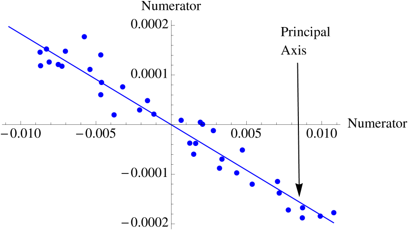
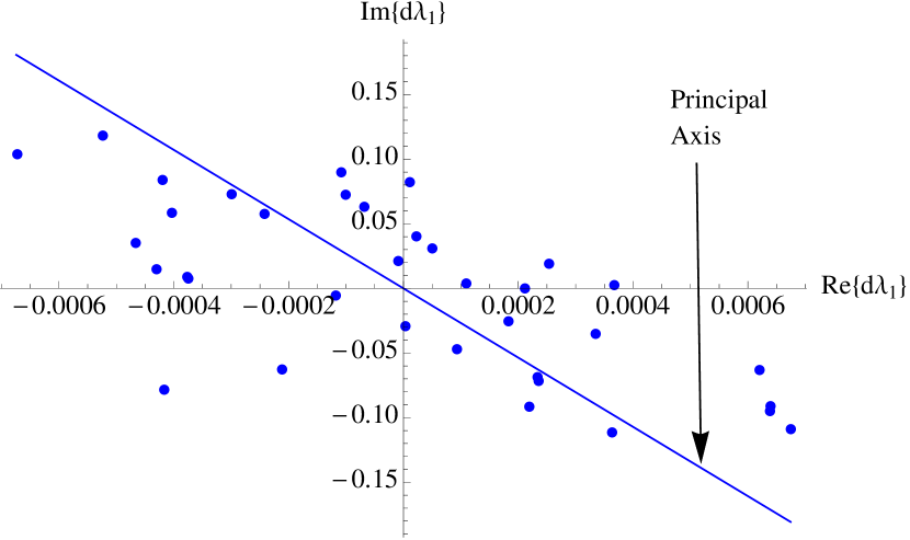
Figure 2: 50 samples of the numerator of (6) and $d\lambda$ after trimming by 30%. Principal axes are computed and shown as lines.

VI-C Ranking generator pairs to damp mode 1

Fig. 3 shows the power flow $p$ and oscillating mode pattern of interarea mode 1 at the base case. The mode pattern shows that generators G2 through G9 are oscillating against G10. The component of G10 is not very large compared with the components of the other generators, but G10 is a large generator that represents an equivalent of the New York State grid. From Fig. 3 we can see that generator G5 participates most in the oscillation, G8 has a small participation in the oscillation, and G1 does not participate in the oscillation.

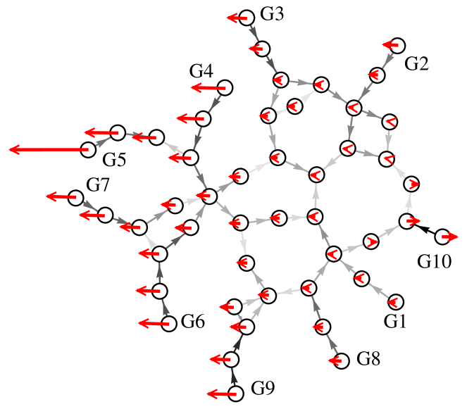
Figure 3: The gray lines joining the buses show the magnitude of the active power flow with the grayscale and the direction of the active power flow with the arrows. The red arrows at each bus show the pattern of the oscillation for mode 1; that is, the magnitude and direction of the entries of the right eigenvector $x_{\delta}$.

The method of section V was applied to rank the generator pairs that best increase the damping ratio for a small redispatch of 0.01 pu, and the top 10 generator pairs are shown in Table VI. The top 9 generator pairs all include G5-; that is, decreasing generation at G5 with increasing generation elsewhere. The change in damping ratio for these pairs are of the same order of magnitude, so it is clear from Table VI that the largest changes in damping ratio are due to the generator pairs involving G5-.

TABLE VI: Generator pairs ranked by change in $\zeta_{1}(\%)$; redispatch = 0.01

Generator Pair	$d\zeta_{1}(\%)$	Generator Pair	$d\zeta_{1}(\%)$
1 G6+,G5-	0.00554	6 G1+,G5-	0.00505
2 G3+,G5-	0.00549	7 G9+,G5-	0.00502
3 G7+,G5-	0.00545	8 G4+,G5-	0.00489
4 G2+,G5-	0.00537	9 G10+,G5-	0.00481
5 G8+,G5-	0.00510	10 G6+,G10-	0.000725

VI-D Ranking generator pairs to damp mode 2

Fig. 4 shows the power flow $p$ and oscillating mode pattern of interarea mode $\lambda_{2}$ at the base case. The mode pattern shows that generators G1-G3 and G6-G9 are oscillating against G5. Generators G5 and G9 participate most in the oscillation.

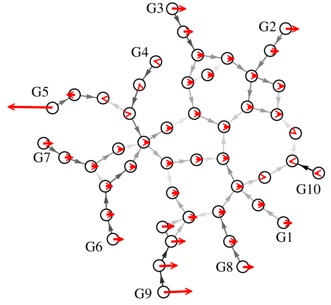
Figure 4: The gray lines joining the buses show the magnitude of the active power flow with the grayscale and the direction of the active power flow with the arrows. The red arrows at each bus show the pattern of the oscillation for mode 2.

The method of section V was applied to rank the generator pairs that best increase the damping ratio for a small redispatch of 0.01 pu, and the top 10 generator pairs are shown in Table VII. The top 9 generator pairs all include G5+; that is, increasing generation at G5 with decreasing generation elsewhere. Although the change in damping ratio is of the same order of magnitude for the 10 pairs, the increase in damping ratio for pair 10 G4+,G9-, is roughly half of the increase of damping ratio for pair 9 G5+,G4-.

Now we analyze the most significant components of formula (6) to explain why G5 is playing a key role in damping mode 2.

TABLE VII: Generator pairs ranked by change in $\zeta_{2}(\%)$; redispatch = 0.01

				Re$\{C_{V}\}$
Gen. Pair	$d\zeta_{2}(\%)$	$d\lambda$	Re$\{C_{\theta}\}\cdot d\theta$	$\cdot\,dV$
1 G5+,G9-	9.60E-3	-4.23E-4 - j0.008	-3.04E-4	-1.19E-4
2 G5+,G8-	7.30E-3	-3.06E-4 - j0.010	-2.23E-4	-8.32E-5
3 G5+,G1-	7.28E-3	-3.02E-4 - j0.011	-2.21E-4	-8.12E-5
4 G5+,G10-	7.26E-3	-3.00E-4 - j0.011	-2.19E-4	-8.10E-5
5 G5+,G2-	6.85E-3	-2.85E-4 - j0.010	-2.10E-4	-7.55E-5
6 G5+,G7-	6.79E-3	-2.84E-4 - j0.010	-2.11E-4	-7.30E-5
7 G5+,G6-	6.77E-3	-2.84E-4 - j0.010	-2.11E-4	-7.28E-5
8 G5+,G3-	6.74E-3	-2.81E-4 - j0.010	-2.08E-4	-7.38E-5
9 G5+,G4-	6.05E-3	-2.52E-4 - j0.009	-1.90E-4	-6.21E-5
10 G4+,G9-	3.53E-3	-1.71E-4 - j0.001	-1.14E-4	-5.66E-5

Table VII shows that the pairs with the largest change in damping ratio $d\zeta$ are the ones with the largest increase in the damping Re$\{d\lambda\}$, so we can focus on the real part of (19). Moreover, Table VII also shows that the changes Re$\{C_{\theta}\}\cdot d\theta$ are larger than the changes Re$\{C_{V}\}\cdot dV$, so we focus on analyzing the terms of (19) related to $d\theta$:

$$\mbox{Re}\{d\lambda\}=\mbox{Re}\{C_{\theta}\}\cdot d\theta+\mbox{Re}\{C_{V}\}\cdot dV\approx\mbox{Re}\{C_{\theta}\}\cdot d\theta$$ (25)

Fig. 5 shows different quantities related to the 56 lines of the New England system in gray scale. Each generator is represented in the network by an internal bus and a terminal bus. There are two lines in series at the edge of the network associated with each generator. The line joining the internal bus to the terminal bus represents the generator transient reactance, and the other line lumps together the transformer and lines joining the generator terminal bus to the network. (G10 differs since it represents New York state.) Fig. 5(a) shows $|\mbox{Re}\{C_{\theta}\}|$, the absolute value of $d\theta$’s coefficient in (25). The lines that represents the transient reactance of G5 and the transient reactance of G9 have large components of $|\mbox{Re}\{C_{\theta}\}|$. Fig. 5(b) shows $|dp|$, the absolute value of the change in power flow in lines for the best ranked generator pair G5+,G9-. As expected, several lines have a significant change in power flow, but Fig. 5(c) shows that only the line that represents the transient reactance of G5 has a large change in angle $|d\theta|$. This is due to the fact that transient reactance of G5 is much larger than the reactance of any of the other 55 lines of the system (see appendix A). So, for any possible generator pair that involves G5, the line that represents the transient reactance of G5 will always have the largest change in angle. This large change in angle, combined with a large coefficient $|\mbox{Re}\{C_{\theta}\}|$, produces the dominant term of (25), as shown by Fig. 5(d). Thus G5 is the key generator to participate in redispatch for producing the largest changes in damping for mode 2. Although Fig. 5(a) shows that there are other lines that have large $d\theta$’s real coefficient, and Fig. 5(b) shows that other lines have an important change in power $|dp|$, Fig. 5(c) shows that such lines do not have a large change in angle $d\theta$, and as a result their associated terms in (25) are not large, as seen in Fig. 5(d). This analysis shows a mechanism of how damping by redispatch works by changing the angles across lines that have large coefficients $C_{\theta}$.

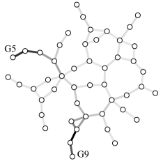
(a) $|\mbox{Re}\{C_{\theta}\}|$ for $\lambda_{2}$.

(b) $|dp|$ for redispatch G5+,G9-.

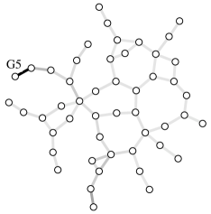
(c) $|d\theta|$ for G5+,G9-.

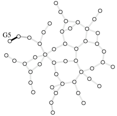
(d) $|\mbox{Re}\{C_{\theta}\}\cdot d\theta|$ for $\lambda_{2}$ & G5+,G9-.

Figure 5: Gray scale in the lines shows the components of the specified vector.

VI-E Larger redispatches

Larger redispatches introduce some nonlinearity in the change in the damping ratio. This nonlinearity arises from three sources: the change in the load flow, the change in the eigenvalue $d\lambda$, and the change in the damping ratio. For a given size of redispatch of a generator pair, we can compute the exact nonlinear change in the load flow due to the redispatch, use (6) to linearly estimate the change in the eigenvalue based on measurements, and then compute the nonlinear change in the damping ratio. This is a large signal application of (6), and the top 10 generator pairs for modes 1 and 2 are shown in Table VIII for a redispatch of 0.4 pu. For comparison, Table VIII also shows the exact calculation that uses the nonlinear computation of $d\lambda$. As shown in Fig. 6, the use of (6) for a larger redispatch gives the same grouping of the top 9 effective generator pairs and a similar ranking and grouping of the top 10 generator pairs as the exact calculation. An exception is that for mode 1, the 5th ranked generator pair G9+,G5- for a larger redispatch using (6) becomes the 9th ranked generator pair for the exact calculation.

Fig. 6 also compares the changes in the damping ratio of the top 10 generator pairs for a small redispatch using (6) to the larger redispatch using (6). The grouping of the top 9 effective generator pairs is preserved and the approximate ranking is preserved.

Overall, some details of the rankings differ for similarly effective generator pairs, but since the ranking will be used to provide a set of effective generators pairs from which an operationally suitable pair can be selected for redispatch by operators, the performance of the ranking is satisfactory.

TABLE VIII: Generator pairs ranked by change in $\zeta(\%)$; redispatch = 0.4

MODE 1	$d\zeta_{1}(\%)$		MODE 2	$d\zeta_{2}(\%)$
Gen. Pair	Using (6)	Exact	Gen. Pair	Using (6)	Exact
1 G6+,G5-	0.181	0.138	1 G5+,G9-	0.563	0.600
2 G7+,G5-	0.177	0.134	2 G5+,G10-	0.558	0.615
3 G3+,G5-	0.177	0.135	3 G5+,G1-	0.534	0.595
4 G2+,G5-	0.171	0.128	4 G5+,G8-	0.506	0.572
5 G9+,G5-	0.162	0.092	5 G5+,G2-	0.473	0.545
6 G4+,G5-	0.160	0.122	6 G5+,G3-	0.453	0.527
7 G8+,G5-	0.159	0.115	7 G5+,G7-	0.434	0.506
8 G1+,G5-	0.155	0.112	8 G5+,G6-	0.432	0.503
9 G10+,G5-	0.145	0.104	9 G5+,G4-	0.365	0.444
10 G6+,G10-	0.030	0.034	10 G4+,G9-	0.139	0.120

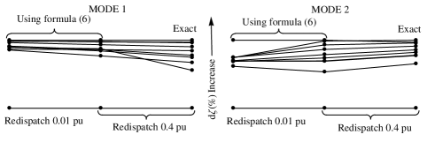
Figure 6: Changes in damping ratio for Mode 1 and Mode 2 for the top 10 generator pairs from Tables VI, VII, VIII rescaled to the same range to allow comparison. For each mode, left hand dots use formula (6) for a small redispatch, middle dots use (6) for a larger redispatch, and the right hand dots are the exact calculation for the larger redispatch. Clustering of similarly effective generator pairs is shown by close dots and changes in ranking appear as lines crossing.

VII Discussion of generator modeling

Since our approach depends in new ways on both measurements and an equivalent second-order swing equation generator model, our generator modeling requirements are different than in other approaches to suppressing oscillations. Section II-C explains that the generator dynamics are approximated by a swing equation, but we do not need to determine the parameters of the swing equation for any individual generator. This section further discusses the generator modeling.

As a general observation, in closed loop control of oscillations with power system stabilizers, which forms most of the literature on suppressing oscillations, the generator and its controls need to be modeled in sufficient detail. Indeed the designed control gains directly affect entries of the Jacobian to damp the oscillatory mode. Our control is open loop and works by the entirely different principle of exploiting system nonlinearity by changing the operating point at which the Jacobian is evaluated. This changes the focus from the linear parts of the model to the nonlinearities.

Formula (6) computes the first order sensitivity of the oscillatory mode eigenvalue to generator redispatch. Appendix B proves that the first order eigenvalue sensitivity to redispatch does not depend on linear parts of the power system model. In particular, if the generator magnetic saturation and hysteresis are neglected, the higher order parts of the generator modeling are linear and the eigenvalue sensitivity only depends on the nonlinearity in the swing equation and any stator algebraic equations and does not depend on the linear higher order part of the generator dynamic modeling. This does suggest that the linear higher order generator dynamics can be omitted in deriving the formula.

In applying formula (6), we do not use a model of the power system dynamics. Instead we rely on measurements of the system dynamics, particularly the eigenvalue and the right eigenvector of the mode and the phase of the complex scalar parameter $\alpha$ that combines together all of the generator dynamics. There are no model assumptions in these measured quantities. That is, if part of the power system affects the oscillatory dynamics, the effect will appear via the measurements used by the formula.

We did an initial test of the approximation involved in generator modeling with the interarea mode of the 3-generator model similar to Fig. 1 with a sixth-order generator model at each bus. Formula (6) is applied to this detailed model by measuring the phase of $\alpha$, and using the computed mode, mode shape, and load flow to estimate the change $d\lambda$ in the eigenvalue that would arise from small redispatches in generation. Then the detailed model is used to compute the exact change $d\lambda$ in the eigenvalue. The comparison of the approximate and exact $d\lambda$ is shown in Table IX. Similarly to the intended application of the formula to ranking redispatches in a real power system, the power system model with sixth-order generators does not have the parameters of the equivalent second order generator models available. That is, the magnitude of $\alpha$ is not known, and only the phase of $\alpha$ is estimated, and so the formula predicts $d\lambda$ to within a constant real multiplier. Therefore in Table IX we compare the ratios of $|d\lambda|$ for each redispatch to $|d\lambda|$ for the redispatch of generators G1 and G2, as well as comparing the phases of $d\lambda$. The approximation of $d\lambda$ in Table IX is close enough to be acceptable for ranking of generator redispatches.

While the generator modeling issues should be investigated further in future work, and further analytic progress is not ruled out, both theoretical considerations of the irrelevance of linear parts of the generator model and an initial test indicate that combining measurements of the dynamic quantities with a formula assuming a second order swing equation can be adequate for ranking generator redispatches.

TABLE IX: Eigenvalue changes for redispatch of 0.01 pu in 3-generator system with sixth-order generator modeling

Generator	Exact		Approximate with formula
pair	$\angle d\lambda$	$|d\lambda|$ ratio	$\angle d\lambda$	$|d\lambda|$ ratio
G1+,G2-	$-109.5^{\circ}$	1.00	$-106.3^{\circ}$	1.00
G2+,G3-	$-98.6^{\circ}$	2.54	$-98.5^{\circ}$	2.12
G1+,G3-	$-101.7^{\circ}$	3.53	$-101.0^{\circ}$	3.11

VIII Conclusions

There has been success in monitoring interarea modal damping with synchrophasor measurements [9, 10]; the next step is to leverage synchrophasor measurements to provide advice to the operators to maintain a suitable modal damping ratio when the damping ratio is insufficient. Difficulties in accomplishing this in the past include the lack of wide-area online dynamic models and standard formulas that depend on quantities that cannot be measured. In this paper, we circumvent these difficulties by calculating the best generator pairs to redispatch to maintain modal damping by combining synchrophasor and state estimator measurements with a new analytic formula for the sensitivity of the mode eigenvalue with respect to generator redispatch. The assumed equivalent generator dynamics only appears as a complex factor $1/\alpha$ common to all redispatches and we propose a method of estimating the phase of $\alpha$ from ambient measurements. The new formula is somewhat complicated, and we explain and illustrate how it works in 3 and 10 generator examples. Future work may well discover further insights and applications using the formula. In summary, we make substantial progress towards practical application of a new formula to damp interarea oscillations based on measurable quantities.

Appendix A: New England generator data

Gen.	Terminal	Internal				$V$ Internal
No.	Bus No.	Bus No.	$h$ [s]	$d$ [s]	$x^{\prime}_{d}$	Bus
1	30	40	42.0	0.0267	0.031	1.0501
2	31	41	30.3	0.0161	0.0697	1.0388
3	32	42	35.8	0.0209	0.0531	1.0439
4	33	43	28.6	0.0243	0.0436	1.0348
5	34	44	26.0	0.0014	0.132	1.2098
6	35	45	34.8	0.0277	0.05	1.0941
7	36	46	26.4	0.0140	0.049	1.0944
8	37	47	24.3	0.0116	0.057	1.0705
9	38	48	34.5	0.0002	0.057	1.1252
10	39	49	500.0	0.3979	0.006	1.0317

$V_{i}$ is the internal constant voltage magnitude of generator $i$ at the base case; i.e., at zero redispatch, and $x^{\prime}_{d}$ is the transient generator reactance.

Appendix B: Irrelevance of linear modeling

This appendix proves from (1) that the first order eigenvalue sensitivity to redispatch does not depend on linear parts of the power system model. This result was first mentioned in [7, section 4.6]. It is convenient to use the extended differential-algebraic form of the power system equations [24] with state vector $z$, Jacobian $\bar{J}$, and extended right and left eigenvectors $\bar{v}$ and $\bar{w}$. In this notation, (1) becomes

$$\frac{\partial\lambda}{\partial p}=\frac{\bar{w}\bar{J}_{p}\bar{v}}{\bar{w}\bar{v}}$$ (26)

In this case, the parameter $p$ parameterizes the generator redispatch, and it appears linearly in the system equations. Therefore $p$ does not appear explicitly in the Jacobian $\bar{J}$, and

$$\bar{J}_{p}=\frac{\partial\bar{J}}{\partial p}=\sum_{k}\frac{\partial\bar{J}}{\partial z^{k}}z_{p}^{k}$$ (27)

where $z_{p}=\frac{\partial z}{\partial p}$ is the sensitivity of the operating point $z$ to the redispatch. Then substituting in (26) and writing it out in coordinates gives

$$\frac{\partial\lambda}{\partial p}=\frac{\displaystyle\sum_{i,j,k}\bar{w}^{i}\frac{\partial\bar{J}^{ij}}{\partial z^{k}}z_{p}^{k}\bar{v}^{j}}{\displaystyle\sum_{i}\bar{w}^{i}\bar{v}^{i}}$$ (28)

It is clear from (28) that the linear parts of the model vanish in $\frac{\partial\bar{J}^{ij}}{\partial z^{k}}$ and that if a dynamic state is associated with a linear differential equation, the corresponding entry of $\bar{w}$ gets multiplied by zero in the numerator of (28).

Sarai Mendoza-Armenta (M 13) received the PhD in Physics from Instituto de Física y Matemáticas, Universidad Michoacana, Mexico in 2013. She was visiting scholar at Iowa State University from March 2012 to March 2013. She was post-doctoral research associate in the Electrical and Computer Engineering Department at Iowa State University.

Ian Dobson (F 06) received the BA in Maths from Cambridge University and the PhD in Electrical Engineering from Cornell University. He previously worked for British industry and the University of Wisconsin-Madison and is currently Sandbulte professor of engineering at Iowa State University.

References

- [1] Cigré Task Force 07 of Advisory Group 01 of Study Committee 38, Analysis and control of power system oscillations, Paris, Dec. 1996.
- [2] G. Rogers, Power System Oscillations, Kluwer Academic, 2000.
- [3] IEEE Power system engineering committee, Eigenanalysis and frequency domain methods for system dynamic performance, IEEE Publication 90TH0292-3-PWR, 1989.
- [4] IEEE PES Systems Oscillations Working Group, Inter-area oscillations in power systems, IEEE Publication 95 TP 101, Oct. 1994.
- [5] C.Y. Chung, L. Wang, F. Howell, P. Kundur, Generation rescheduling methods to improve power transfer capability constrained by small-signal stability, IEEE Trans. Power Syst., vol. 19, no. 1, pp. 524-530, Feb. 2004.
- [6] Z. Huang, N. Zhou, F.K. Tuffner, Y. Chen, D.J. Trudnowski, MANGO-Modal analysis for grid operation: A method for damping improvement through operating point adjustment, U.S. Dept. of Energy, Oct. 2010.
- [7] I. Dobson, F.L. Alvarado, C.L. DeMarco, P. Sauer, S. Greene, H. Engdahl, J. Zhang, Avoiding and suppressing oscillations, PSerc publication 00-01, Dec. 1999.
- [8] A. Fischer, I. Erlich, Assessment of power system small signal stability based on mode shape information, IREP Bulk Power System Dynamics and Control V, Onomichi, Japan, Aug. 2001.
- [9] J.W. Pierre, D.J. Trudnowski, M.K. Donnelly, Initial results in electromechanical mode identification from ambient data, IEEE Trans. Power Syst., vol. 12, no. 3, pp. 1245-1251, Aug. 1997.
- [10] R.W. Wies, J.W. Pierre, D.J. Trudnowski, Use of ARMA block processing for estimating stationary low-frequency electromechanical modes of power systems, IEEE Trans. Power Syst., vol. 18, no. 1, pp. 167-173, Feb. 2003.
- [11] S. Mendoza-Armenta, I. Dobson, A formula for damping interarea oscillations with generator redispatch, IREP Symposium - Bulk Power System Dynamics and Control - IX Rethymnon, Greece, Aug. 2013. Also available online arXiv:1306.3590v2.
- [12] A. Fischer, I. Erlich, Impact of long-distance power transits on the dynamic security of large interconnected power systems, IEEE Porto Power Tech Conference, Porto, Portugal, Sept. 2001.
- [13] D.J. Trudnowski, Estimating electromechanical mode shape from synchrophasor measurements, IEEE Trans. Power Syst., vol. 23, no. 3, pp. 1188-1195, Aug. 2008.
- [14] N.R. Chaudhuri, B. Chaudhuri, Damping and relative mode-shape estimation in near real-time through phasor approach, IEEE Trans. Power Syst., vol. 26, no. 1, pp. 364-373, Feb. 2011.
- [15] L. Dosiek, N. Zhou, J.W. Pierre, Z. Huang, D.J. Trudnowski, Mode shape estimation algorithms under ambient conditions: A comparative review, IEEE Trans. Power Syst., vol. 28, no. 2, pp. 779-787, May 2013.
- [16] E. Barocio, B. C. Pal, N. F. Thornhill, A. R. Messina, A dynamic mode decomposition framework for global power system oscillation analysis, IEEE Trans. Power Syst., vol. PP, issue: 99, 2014.
- [17] Z. Huang, N. Zhou, F. Tuffner, Y. Chen, D. Trudnowski, W. Mittelstadt, J. Hauer, J. Dagle, Improving small signal stability through operating point adjustment, IEEE PES General Meeting, Minneapolis, MN, July 2010.
- [18] R. Diao, Z. Huang, N. Zhou, Y. Chen, F. Tuffner, J. Fuller, S. Jin, J.E Dagle, Deriving optimal operational rules for mitigating inter-area oscillations, Power Syst. Conf. & Exposition, Phoenix AZ, March 2011.
- [19] I. Dobson, F.L. Alvarado, C.L. DeMarco, Sensitivity of Hopf bifurcations to power system parameters, 31st Conference on Decision and Control, Tucson, Arizona, Dec. 1992.
- [20] H.K. Nam, Y.K. Kim, K.S. Shim, K.Y. Lee, A new eigen-sensitivity theory of augmented matrix and its applications to power system stability, IEEE Trans. Power Syst., vol. 15, pp. 363-369, Feb. 2000.
- [21] S. Wang, Q. Jiang, Y. Cao, WAMS-based monitoring and control of Hopf bifurcations in multi-machine power systems, Journal of Zhejiang University Science A, vol. 9, No. 6, pp. 840-848, 2008.
- [22] B.E. Eliasson, D.J. Hill, Damping structure and sensitivity in the Nordel power system, IEEE Trans. Power Syst., vol. 7, No. 1, Feb. 1992.
- [23] E. Mallada, A. Tang, Improving damping of power networks: power scheduling and impedance adaptation, Conf. Decision and Control and European Control Conf. (CDC-ECC), Orlando, FL, Dec. 2011.
- [24] T. Smed, Feasible eigenvalue sensitivity for large power systems, IEEE Transactions on Power Systems, Vol. 8, No. 2, pp. 555-563, May 1993.
- [25] A. Chakrabortty, J. H. Chow, A. Salazar, A measurement-based framework for dynamic equivalencing of large power systems using WAMS, Innovative Smart Grid Technologies, Gaithersburg, MD, Jan. 2010.
- [26] N. Zhou, S. Lu, R. Singh, M. Elizondo, Calibration of reduced dynamic models of power systems using phasor measurement unit (PMU) data, North American Power Symp. (NAPS), Boston MA, Aug. 2011.
- [27] L. Vanfretti, J.H. Chow, Analysis of power system oscillations for developing synchrophasor data applications, IREP Symposium Bulk Power System Dynamics and Control VIII, Buzios, Brazil, Aug. 2010.
- [28] IEEE Task Force on Identification of Electromechanical Modes, Identification of electromechanical modes in power systems, IEEE Special Publication TP462, June 2012.
- [29] G. Liu, J. Ning, Z. Tashman, V. Venkatasubramanian, P. Trachian, Oscillation monitoring system using synchrophasors, IEEE Power and Energy Society General Meeting, San Diego CA, July 2012.
- [30] J. Ning, X. Pan, V. Venkatasubramanian, Oscillation modal analysis from ambient synchrophasor data using distributed frequency domain optimization, IEEE Trans. Power Systems, vol. 28, no. 2, 2013, pp. 1960-1968.
- [31] H. Khalilinia, L. Zhang, V. Venkatasubramanian, Fast frequency-domain decomposition for ambient oscillation monitoring, IEEE Trans. Power Delivery, vol. 30, no. 3, pp: 1631-1633, June 2015.
- [32] M. A. Pai, Energy function analysis for power system stability, Kluwer, Norwell, MA, 1989.
- [33] Y. Zuo, Multidimensional trimming based on projection depth, Annals of Statistics, Vol. 34, No. 5, pp. 2211-2251, Oct. 2006.