An Optimal Control Approach for the Data Harvesting Problem

Abstract

We propose a new method for trajectory planning to solve the data harvesting problem. In a two-dimensional mission space, $N$ mobile agents are tasked with the collection of data generated at $M$ stationary sources and delivery to a base aiming at minimizing expected delays. An optimal control formulation of this problem provides some initial insights regarding its solution, but it is computationally intractable, especially in the case where the data generating processes are stochastic. We propose an agent trajectory parameterization in terms of general function families which can be subsequently optimized on line through the use of Infinitesimal Perturbation Analysis (IPA). Explicit results are provided for the case of elliptical and Fourier series trajectories and some properties of the solution are identified, including robustness with respect to the data generation processes and scalability in the size of an event set characterizing the underlying hybrid dynamic system.

I Introduction

Systems consisting of cooperating mobile agents are being continuously developed for a broad spectrum of applications such as environmental sampling [1],[2], surveillance [3], coverage control [4],[5],[6], persistent monitoring [7],[8], task assignment [9], and data harvesting and information collection [10],[11],[12]. The data harvesting problem arises in many settings, including “smart cities” where wireless sensor networks (WSNs) are being widely deployed for purposes of monitoring the environment, traffic, infrastructure for transportation and for energy distribution, surveillance, and a variety of other specialized purposes [13]. Although many efforts focus on the analysis of the vast amount of data gathered, we must first ensure the existence of robust means to collect all data in a timely fashion when the size of the sensor networks and the level of node interference do not allow for a fully wireless connected system. Sensors can locally gather and buffer data, while mobile elements (e.g., vehicles, aerial drones) retrieve the data from each part of the network. Similarly, mobile elements may themselves be equipped with sensors and visit specific points of interest to collect data which must then be delivered to a given base. These mobile agents should follow an optimal path (in some sense to be defined) which allows visiting each data source frequently enough and within the constraints of a given environment like that of an urban setting.

The data harvesting problem using mobile agents known as “message ferries” or “data mules” has been considered from several different perspectives. For a survey on different routing problems in WSNs see [14],[15] and references therein. In [16] algorithms are proposed for patrolling target points with the goal of balanced time intervals between consecutive visits. A weighted version of the algorithm improves the performance in cases with unequally valued targets. However, in this scenario the data need not be delivered to a base and visits to a recharging station are only necessary if the data mules are running out of energy. In [11] the problem is viewed as a polling system with a mobile server visiting data queues at fixed targets. Trajectories are designed for the mobile server in order to stabilize the system, keeping queue contents (modeled as fluid queues) uniformly bounded.

In this paper, we consider the data harvesting problem as an optimal control problem for a team of multiple cooperating mobile agents responsible for collecting data generated by arbitrary random processes at fixed target points and delivering these data to a base. The ultimate goal is for the data to be collected and delivered with minimum expected delay. Rather than looking at this problem as a scheduling task where visit times for each target are determined assuming agents only move in straight lines between targets, we aim to optimize a two-dimensional trajectory for each agent, which may be periodic and can collect data from a target once the agent is within a given range from that target. Interestingly, the setting of the problem can also be viewed as an evacuation process where visits are needed to retrieve individuals from a set of target points which may be of non-uniform importance. In this paper, we limit ourselves to trajectories with no constraints due to obstacles or other factors. Clearly, in an urban environment this is generally not the case and the set of admissible trajectories will have to be restricted in subsequent work.

We formulate a finite-horizon optimal control problem in which the underlying dynamic system has hybrid (time-driven and event-driven) dynamics. We note that the specification of an appropriate objective function is nontrivial for the data harvesting problem, largely due to the fact that the agents act as mobile servers for the data sources and have their own dynamics. Since the control is applied to the motion of agents, the objective function must capture the agent behavior in addition to that of the data queues at the targets, the agents, and the base. The solution of this optimal control problem (even in the deterministic case) requires a Two Point Boundary Value Problem (TPBVP) numerical solver which is clearly not suited for on-line operation and yields only locally optimal solutions. Thus, the main contribution of the paper is to formulate and solve an optimal parametric agent trajectory problem. In particular, similar to the idea in [17] we represent an agent trajectory in terms of general function families characterized by a set of parameters that we seek to optimize, given an objective function. We consider elliptical trajectories as well as the much richer set of Fourier series trajectory representations. We then show that we can make use of Infinitesimal Perturbation Analysis (IPA) for hybrid systems [18] to determine gradients of the objective function with respect to these parameters and subsequently obtain (at least locally) optimal trajectories. This approach also allows us to exploit $(i)$ robustness properties of IPA to allow stochastic data generation processes, $(ii)$ the event-driven nature of the IPA gradient estimation process which is scalable in the event set of the underlying hybrid dynamic system, and $(iii)$ the on-line computation which implies that trajectories adjust as operating conditions change (e.g., new targets).

In section II we present an optimal control formulation for the data harvesting problem. In section III we provide a Hamiltonian analysis leading to a TPBVP. In section IV we formulate the alternative problem of determining optimal trajectories based on general function representations and provide solutions using a gradient-based algorithm using IPA for two particular function families. Sections V and VI present the numerical results and the conclusions respectively.

II Problem Formulation

We consider a data harvesting problem where $N$ mobile agents collect data from $M$ stationary targets in a two-dimensional rectangular mission space $S=[0,L_{1}]\times[0,L_{2}]\subset\mathbbm{R}^{2}$. Each agent may visit one or more of the $M$ targets, collect data from them, and deliver them to a base. It then continues visiting targets, possibly the same as before or new ones, and repeats this process. By cooperating in how data are collected and delivered, the objective of the agent team is to minimize a weighted sum of collection and delivery delays over all targets.

Let $s_{j}(t)=[s_{j}^{x}(t),s_{j}^{y}(t)]$ be the position of agent $j$ at time $t$ with $s_{j}^{x}(t)\in[0,L_{1}]$ and $s_{j}^{y}(t)\in[0,L_{2}]$. The position of the agent follows single integrator dynamics:

$$\dot{s}_{j}^{x}(t)=u_{j}(t)\cos\theta_{j}(t),\quad\ \ \dot{s}_{j}^{y}(t)=u_{j}(t)\sin\theta_{j}(t)$$ (1)

where $u_{j}(t)$ is the scalar speed of the agent (normalized so that $0\leq u_{j}(t)\leq 1$) and $\theta_{j}(t)$ is the angle relative to the positive direction, $0\leq\theta_{j}(t)<2\pi$. Thus, we assume that the agent controls its orientation and speed. An agent is represented as a particle, so that we will omit the need for any collision avoidance control. The agent dynamics above could be more complicated without affecting the essence of our analysis, but we will limit ourselves here to (1).

Consider a set of data sources as points $w_{i}\in S,$ $i=1,\dots,M,$ with associated ranges $r_{ij}$, so that agent $j$ can collect data from $w_{i}$ only if the Euclidean distance $D_{ij}(t)=\|w_{i}-s_{j}(t)\|$ satisfies $D_{ij}(t)\leq r_{ij}$. Similarly, there is a base at $w_{\!{}_{B}}\in S$ which receives all data collected by the agents. An agent can only deliver data to the base if the Euclidean distance $D_{\!{}_{Bj}}(t)=\|w_{\!{}_{Bj}}-s_{j}(t)\|$ satisfies $D_{\!{}_{Bj}}(t)\leq r_{Bj}$. We define a function $P_{ij}(t)$ to be the normalized data collection rate from target $i$ when the agent is at $s_{j}(t)$:

$$P_{ij}(t)=p(w_{i},s_{j}(t))$$ (2)

and we assume that: $({\bf A1})$ it is monotonically non-increasing in the value of $D_{ij}(t)=\|w_{i}-s_{j}(t)\|$, and $({\bf A2})$ it satisfies $P_{ij}(t)=0$ if $D_{ij}(t)>r_{ij}$. Thus, $P_{ij}(t)$ can model communication power constraints which depend on the distance between a data source and an agent equipped with a receiver (similar to the model used in [11]) or sensing range constraints if an agent collects data using on-board sensors. For simplicity, we will also assume that: $({\bf A3})$ $P_{ij}(t)$ is continuous in $D_{ij}(t)$. Similarly, we define:

$$P_{\!{}_{Bj}}(t)=p(w_{\!{}_{B}},s_{j}(t))$$ (3)

Figure 1: Data harvesting queueing model for $M$ targets and $N$ agents

The data harvesting problem described above can be viewed as a polling system where mobile agents are serving the targets by collecting data and delivering them to the base. Figure 1 shows a queueing system in which each $P_{ij}(t)$ is depicted as a switch activated when $D_{ij}(t)\leq r_{ij}$ to capture the finite range between agent $j$ and target $i$. All queues are modeled as flow systems whose dynamics are given next (however, as we will see, the agent trajectory optimization is driven by events observed in the underlying system where queues contain discrete data packets so that this modeling device has minimal effect on our analysis). As seen in Fig. 1, there are three sets of queues. The first set includes the data contents $X_{i}(t)\in\mathbb{R}^{+}$ at each target $i=1,...,M$ where we use $\sigma_{i}(t)$ as the instantaneous inflow rate. In general, we treat $\{\sigma_{i}(t)\}$ as a random process assumed only to be piecewise continuous; we will treat it as a deterministic constant only for the Hamiltonian analysis in the next section. Thus, at time $t$, $X_{i}(t)$ is a random variable resulting from the random process $\{\sigma_{i}(t)\}$. The second set of queues consists of data contents $Z_{ij}(t)\in\mathbb{R}^{+}$ onboard agent $j$ collected from target $i$ as long as $P_{ij}(t)>0$. The last set consists of queues $Y_{i}(t)\in\mathbb{R}^{+}$ containing data at the base, one queue for each target, delivered by some agent $j$ as long as $P_{\!{}_{Bj}}(t)>0$. Note that $\{X_{i}(t)\}$, $\{Z_{ij}(t)\}$ and $\{Y_{i}(t)\}$ are also random processes and the same applies to the agent states $\{s_{j}(t)\}$, $j=1,\dots,N$, since the controls are generally dependent on the random queue states. Thus, we ensure that all random processes are defined on a common probability space. The maximum rate of data collection from target $i$ by agent $j$ is $\mu_{ij}$ and the actual rate is $\mu_{ij}P_{ij}(t)$ if $j$ is connected to $i$. We will assume that: $({\bf A4})$ only one agent at a time is connected to a target $i$ even if there are other agents $l$ with $P_{il}(t)>0$; this is not the only possible model, but we adopt it based on the premise that simultaneous downloading of packets from a common source creates problems of proper data reconstruction at the base. The dynamics of $X_{i}(t)$, assuming that agent $j$ is connected to it, are

$$\dot{X}_{i}(t)=\left\{\begin{array}[c]{ll}0\qquad\quad\mbox{if }X_{i}(t)=0\mbox{ and }\sigma_{i}(t)\leq\mu_{ij}(t)P_{ij}(t)\\ \sigma_{i}(t)-\mu_{ij}(t)P_{ij}(t)\quad\qquad\qquad\qquad\mbox{otherwise}\end{array}\right.$$ (4)

Obviously, $\dot{X}_{i}(t)=\sigma_{i}(t)$ if $P_{ij}(t)=0$, $j=1,\dots,N$. In order to express the dynamics of $Z_{ij}(t)$, let

This gives us the dynamics:

where $\beta_{ij}$ is the maximum rate of data from target $i$ delivered by agent $j$. For simplicity, we assume that: $({\bf A5})$ $\|w_{i}-w_{B}\|>r_{ij}+r_{Bj}$ for all $i=1,\dots,M$ and $j=1,\dots,N$, i.e., the agent cannot collect and deliver data at the same time. Therefore, in (6) it is always the case that $P_{ij}(t)P_{Bj}(t)=0$. Finally, the dynamics of $Y_{i}(t)$ depend on $Z_{ij}(t)$, the content of the on-board queue of each agent $j$ from target $i$ as long as $P_{Bj}(t)>0$. We define $\beta_{i}(t)=\sum_{j=1}^{N}\beta_{ij}P_{Bj}(t)\mathbf{1}[Z_{ij}(t)>0]$ to be the total instantaneous delivery rate for target $i$ data, so that the dynamics of $Y_{i}(t)$ are:

$$\dot{Y}_{i}(t)=\beta_{i}(t)$$ (7)

Our objective is to maintain minimal values for all target and on-board agent data queues, while maximizing the contents of the delivered data at the base queues. Thus, we define $J_{1}(X_{1},\ldots,X_{M},t)$ to be the weighted sum of expected target queue contents (recalling that $\{\sigma_{i}(t)\}$ are random processes):

$$J_{1}(X_{1},\ldots X_{M},t)=\sum\limits_{i=1}^{M}q_{i}E[X_{i}(t)]$$ (8)

where the weight $q_{i}$ represents the importance factor of target $i$. Similarly, we define a weighted sum of expected base queues contents:

$$J_{2}(Y_{1},\ldots Y_{M},t)=\sum\limits_{i=1}^{M}q_{i}E[Y_{i}(t)]$$ (9)

For simplicity, we will in the sequel assume that $q_{i}=1$ for all $i$ without affecting any aspect of our analysis. Therefore, our optimization objective may be a convex combination of (8) and (9). In addition, we need to ensure that the agents are controlled so as to maximize their utilization, i.e., the fraction of time spent performing a useful task by being within range of a target or the base. Equivalently, we aim to minimize the non-productive idling time of each agent during which it is not visiting any target or the base. Let

so that the idling time for agent $j$ occurs when $D_{ij}^{+}(t)>0$ for all $i$ and $D_{Bj}^{+}(t)>0$. We define the idling function $I_{j}(t)$:

$$I_{j}(t)=\log\Bigg{(}1+D_{\!{}_{Bj}}^{+}(t)\prod_{i=1}^{M}D_{ij}^{+}(t)\Bigg{)}$$ (11)

This function has the following properties. First, $I_{j}(t)=0$ if and only if the product term inside the bracket is zero, i.e., agent $j$ is visiting a target or the base; otherwise, $I_{j}(t)>0$. Second, $I_{j}(t)$ is monotonically nondecreasing in the number of targets $M$. The logarithmic function is selected so as to prevent the value of $I_{j}(t)$ from dominating those of $J_{1}(\cdot)$ and $J_{2}(\cdot)$ when included in a single objective function. We define:

$$J_{3}(t)=M_{I}\sum\limits_{j=1}^{N}E[I_{j}(t)]$$ (12)

where $M_{I}$ is a weight for the idling time effect relative to $J_{1}(\cdot)$ and $J_{2}(\cdot)$. Note that $I_{j}(t)$ is also a random variable since it is a function of the agent states $s_{j}(t)$, $j=1,\dots,N$. Finally, we define a terminal cost at $T$ capturing the expected value of the amount of data left on board the agents, noting that the effect of this term vanishes as $T$ goes to infinity as long as all $E[Z_{ij}(T)]$ remain bounded:

$$J_{f}(T)=\frac{1}{T}\sum\limits_{i=1}^{M}\sum\limits_{j=1}^{N}E[Z_{ij}(T)]$$ (13)

We can now formulate a stochastic optimization problem $\mathbf{P1}$ where the control variables are the agent speeds and headings denoted by the vectors $\mathbf{u}(t)=[u_{1}(t),\dots,u_{N}(t)]$ and $\boldsymbol{\theta}(t)=[\theta_{1}(t),\dots,\theta_{N}(t)]$ respectively (omitting their dependence on the full system state at $t$). We combine the objective function components in (8), (9), (12) and (13) to obtain:

where $\alpha\in[0,1]$ is a weight capturing the relative importance of collected data as opposed to delivered data and $0\leq u_{j}(t)\leq 1$, $0\leq\theta_{j}(t)<2\pi$. To simplify notation, we have also expressed $J_{1}(X_{1},\ldots X_{M},t)$ and $J_{2}(Y_{1},\ldots Y_{M},t)$ as $J_{1}(t)$ and $J_{2}(t)$.

Since we are considering a finite time optimization problem, instability in the queues is not an issue. However, stability of such a system can indeed be an issue in the sense of guaranteeing that $E[X_{i}(t)]<\infty$, $E[Z_{ij}(T)]<\infty$ for all $i,j$ under a particular control policy when $t\to\infty$. This problem is considered in [11] for a simpler deterministic data harvesting model where target queues are required to be bounded. In this paper, we do not explicitly study this issue; however, given a certain number of agents, it is possible to stabilize a target queue by designing agent trajectories to ensure that the queue is visited frequently enough and periodically emptied.

III Optimal Control Solution

In this section, we address $\mathbf{P1}$ in a setting where all data arrival processes are deterministic, so that all expectations in (8)-(13) degenerate to their arguments. We proceed with a standard Hamiltonian analysis leading to a Two Point Boundary Value Problem (TPBVP) [19] where the states and costates are known at $t=0$ and $t=T$ respectively. We define a state vector and the associated costate vector:

$$\begin{split}\mathbf{X}&(t)=[X_{1}(t),\dots,X_{M}(t),Y_{1}(t),\dots,Y_{M}(t),\\ &Z_{11}(t),\dots,Z_{MN}(t),s_{1}^{x}(t),s_{1}^{y}(t),\dots,s_{N}^{x}(t),s_{N}^{y}(t)]\end{split}$$

$$\begin{split}\boldsymbol{\lambda}&(t)=[\lambda_{1}(t),\dots,\lambda_{M}(t),\gamma_{1}(t),\dots,\gamma_{M}(t),\\ &\phi_{11}(t),\dots,\phi_{MN}(t),\eta_{1}^{x}(t),\eta_{1}^{y}(t),\dots,\eta_{N}^{x}(t),\eta_{N}^{y}(t)]\end{split}$$

The Hamiltonian is

where the costate equations are

$$\begin{array}[c]{ll}\dot{\lambda}_{i}(t)=-\frac{\partial H}{\partial{X_{i}}}=-\frac{\alpha}{T}&\lambda_{i}(T)=0\\ \dot{\gamma}_{i}(t)=-\frac{\partial H}{\partial{Y_{i}}}=\frac{1-\alpha}{T}&\gamma_{i}(T)=0\\ \dot{\phi}_{ij}(t)=-\frac{\partial H}{\partial{Z_{ij}}}=0&\phi_{ij}(T)=\frac{\partial J_{f}(t)}{\partial Z_{ij}}\Big{|}_{T}\end{array}$$

$$\eta_{j}^{x}(T)=\eta_{j}^{y}(T)=0$$

From (15), after some trigonometric manipulations, we get

where $\tan\psi_{j}(t)=\frac{\eta_{j}^{x}(t)}{\eta_{j}^{y}(t)}$ for $\eta_{j}^{y}(t)\neq 0$ and $\psi_{j}(t)=\mbox{sgn}(\eta_{j}^{x}(t))\frac{\pi}{2}$ if $\eta_{j}^{y}(t)=0$. Applying the Pontryagin principle to (15) with $(\mathbf{u}^{\ast},{\boldsymbol{\theta}}^{\ast})$ being the optimal control, we have:

$$H(\mathbf{X}^{\ast},{\boldsymbol{\lambda}}^{\ast},\mathbf{u}^{\ast},{\boldsymbol{\theta}}^{\ast})=\min\limits_{\mathbf{u}(t),\boldsymbol{\theta}(t)}H(\mathbf{X},{\boldsymbol{\lambda}},\mathbf{u},{\boldsymbol{\theta}})$$ (18)

From (17) we easily see that we can always make the $u_{j}(t)$ multiplier to be negative, hence, recalling that $0\leq u_{j}(t)\leq 1$,

$$u_{j}^{\ast}(t)=1$$ (19)

Following the Hamiltonian definition in (15) we have:

$$\frac{\partial H}{\partial\theta_{j}}=-\eta_{j}^{x}(t)u_{j}(t)\sin\theta_{j}(t)+\eta_{j}^{y}(t)u_{j}(t)\cos\theta_{j}(t)$$ (20)

and setting $\frac{\partial H}{\partial\theta_{j}}=0$ the optimal heading $\theta_{j}^{\ast}(t)$ should satisfy:

$$\tan\theta_{j}^{\ast}(t)=\frac{{\eta_{j}^{y}}(t)}{{\eta_{j}^{x}}(t)}$$ (21)

Since $u_{j}^{\ast}(t)=1$, we only need to evaluate $\theta_{j}^{\ast}(t)$ for all $t\in[0,T]$. This is accomplished by discretizing the problem in time and numerically solving a TPBVP with a forward integration of the state and a backward integration of the costate. Solving this problem quickly becomes intractable as the number of agents and targets grows. However, one of the insights this analysis provides is that under optimal control the data harvesting process operates as a hybrid system with discrete states (modes) defined by the dynamics of the flow queues in (4), (6), (7), while the agents maintain a fixed speed. The events that trigger mode transitions are defined in Table I (the superscript $0$ denotes events causing a variable to reach a value of zero from above and the superscript $+$ denotes events causing a variable to become strictly positive from a zero value):

TABLE I: Hybrid System Events

Event Name	Description
1. $\xi_{i}^{0}$	$X_{i}(t)$ hits 0, for $i=1,\dots,M$
2. $\xi_{i}^{+}$	$X_{i}(t)$ leaves 0, for $i=1,\ldots,M$.
3. $\zeta_{ij}^{0}$	$Z_{ij}(t)$ hits 0, for $i=1,\ldots,M$, $j=1,\ldots,N$
4. $\delta_{ij}^{+}$	$D_{ij}^{+}(t)$ leaves 0, for $i=1,\ldots,M$, $j=1,\ldots,N$
5. $\delta_{ij}^{0}$	$D_{ij}^{+}(t)$ hits 0, for $i=1,\ldots,M$, $j=1,\ldots,N$
6. $\Delta_{j}^{+}$	$D_{\!{}_{Bj}}^{+}(t)$ leaves 0, for $j=1,\ldots,N$
7. $\Delta_{j}^{0}$	$D_{\!{}_{Bj}}^{+}(t)$ hits 0, for $j=1,\ldots,N$

Observe that each of these events causes a change in at least one of the state dynamics in (4), (6), (7). For example, $\xi_{i}^{0}$ causes a switch in (4) from $\dot{X}_{i}(t)=\sigma_{i}(t)-\mu_{ij}P_{ij}(t)$ to $\dot{X}_{i}(t)=0$. Also note that we have omitted an event $\zeta_{ij}^{+}$ for $Z_{ij}(t)$ leaving 0 since this event is immediately induced by $\delta_{ij}^{0}$ when agent $j$ comes within range of target $i$ and starts collecting data causing $Z_{ij}(t)$ to become positive if $Z_{ij}(t)=0$ and $X_{i}(t)>0$. Finally, note that all events above are directly observable during the execution of any agent trajectory and they do not depend on our model of flow queues. For example, if $X_{i}(t)$ becomes zero, this defines event $\xi_{i}^{0}$ regardless of whether the corresponding queue is based on a flow or on discrete data packets; this observation is very useful in the sequel.

The fact that we are dealing with a hybrid dynamic system further complicates the solution of a TPBVP. On the other hand, it enables us to make use of Infinitesimal Perturbation Analysis (IPA) [18] to carry out the parametric trajectory optimization process discussed in the next section. In particular, we propose a parameterization of agent trajectories allowing us to utilize IPA to obtain a gradient of the objective function with respect to the trajectory parameters.

IV Agent Trajectory Parameterization and Optimization

The idea here is to represent each agent’s trajectory through general parametric equations

$$\begin{array}[c]{ll}s_{j}^{x}(t)=f(\Theta_{j},\rho_{j}(t)),\text{ \ }\quad s_{j}^{y}(t)=g(\Theta_{j},\rho_{j}(t))&\end{array}$$ (22)

where the function $\rho_{j}(t)$ controls the position of the agent on its trajectory at time $t$ and $\Theta_{j}$ is a vector of parameters controlling the shape and location of the agent $j$ trajectory. Let $\Theta=[\Theta_{1},\dots,\Theta_{N}]$. We now replace problem $\mathbf{P1}$ in (14) by problem $\mathbf{P2}$:

$$\begin{split}\min\limits_{\Theta\in F_{\Theta}}&\frac{1}{T}\int_{0}^{T}\Big{[}\alpha J_{1}(\Theta,t)-(1-\alpha)J_{2}(\Theta,t)+J_{3}(\Theta,t)\Big{]}dt\\ &+J_{f}(\Theta,T)\end{split}$$ (23)

where we return to allowing arbitrary stochastic data arrival processes $\{\sigma_{i}(t)\}$ so that $\mathbf{P2}$ is a parametric stochastic optimization problem with $F_{\Theta}$ appropriately defined depending on (22). The cost function in (23) is written as

$$J(\Theta,T;\mathbf{X}(\Theta,0))=E[\mathcal{L}(\Theta,T;\mathbf{X}(\Theta,0))]$$

where $\mathcal{L}(\Theta,T;\mathbf{X}(\Theta,0))$ is a sample function defined over $[0,T]$ and $\mathbf{X}(\Theta,0)$ is the initial value of the state vector. For convenience, in the sequel we will use $\mathcal{L}_{1}$, $\mathcal{L}_{2}$, $\mathcal{L}_{3}$, $\mathcal{L}_{f}$ to denote sample functions of $J_{1}$, $J_{2}$, $J_{3}$ and $J_{f}$ respectively. Note that in (23) we suppress the dependence of the four objective function components on the controls $\mathbf{u}(t)$ and $\boldsymbol{\theta}(t)$ and stress instead their dependence on the parameter vector $\Theta$. In the rest of the paper, we will consider two families of trajectories motivated by a similar approach used in the multi-agent persistent monitoring problem in [20]: elliptical trajectories and a Fourier series trajectory representation which is more general and better suited for non-uniform target topologies. The hybrid dynamics of the data harvesting system allow us to apply the theory of IPA [18] to obtain on line the gradient of the sample function $\mathcal{L}(\Theta,T;\mathbf{X}(\Theta,0))$ with respect to $\Theta$. The value of the IPA approach is twofold: $(i)$ The sample gradient $\nabla\mathcal{L}(\Theta,T)$ can be obtained on line based on observable sample path data only, and $(ii)$ $\nabla\mathcal{L}(\Theta,T)$ is an unbiased estimate of $\nabla J(\Theta,T)$ under mild technical conditions as shown in [18]. Therefore, we can use $\nabla\mathcal{L}(\Theta,T)$ in a standard gradient-based stochastic optimization algorithm

$$\Theta^{l+1}=\Theta^{l}-\boldsymbol{\nu}_{l}\nabla\mathcal{L}(\Theta^{l},T),\text{ \ }l=0,1,\ldots$$ (24)

to converge (at least locally) to an optimal parameter vector $\Theta^{\ast}$ with a proper selection of a step-size sequence $\{\boldsymbol{\nu}_{l}\}$ [21]. We emphasize that this process is carried out on line, i.e., the gradient is evaluated by observing a trajectory with given $\Theta$ over $[0,T]$ and is iteratively adjusting it until convergence is attained.

IV-1 IPA equations

Based on the events defined earlier, we will specify event time derivative and state derivative dynamics for each mode of the hybrid system. In this process, we will use the IPA notation from [18] so that ${\tau_{k}}$ is the $k$th event time in an observed sample path of the hybrid system and ${\tau_{k}^{{}^{\prime}}}=\frac{d\tau_{k}}{d\Theta}$, $\mathcal{X}^{\prime}(t)=\frac{d\mathcal{X}}{d\Theta}$ are the Jacobian matrices of partial derivatives with respect to all components of the controllable parameter vector $\Theta$. Throughout the analysis we will be using $(\cdot)^{\prime}$ to show such derivatives. We will also use $f_{k}(t)=\frac{d\mathcal{X}}{dt}$ to denote the state dynamics in effect over an interevent time interval $[{\tau_{k},\tau_{k+1})}$. We review next the three fundamental IPA equations from [18] based on which we will proceed. First, events may be classified as exogenous or endogenous. An event is exogenous if its occurrence time is independent of the parameter $\Theta$, hence ${\tau_{k}^{{}^{\prime}}}=0$. Otherwise, an endogenous event takes place when a condition $g_{k}(\Theta,\mathcal{X})=0$ is satisfied, i.e., the state $\mathcal{X}(t)$ reaches a switching surface described by $g_{k}(\Theta,\mathcal{X})$. In this case, it is shown in [18] that

$${\tau_{k}^{{}^{\prime}}}=-\Big{(}\frac{dg_{k}}{d\mathcal{X}}f_{k}(\tau_{k}^{-})\Big{)}^{-1}\Big{(}\frac{dg_{k}}{d\Theta}+\frac{dg_{k}}{d\mathcal{X}}{\mathcal{X}^{\prime}(\tau_{k}^{-})}\Big{)}$$ (25)

as long as $\frac{\partial g_{k}}{\partial\mathcal{X}}f_{k}(\tau_{k}^{-})\neq 0$. It is also shown in [18] that the state derivative $\mathcal{X}^{\prime}(t)$ satisfies

$$\frac{d}{dt}\mathcal{X}^{\prime}(t)=\frac{df_{k}}{d\mathcal{X}}\mathcal{X}^{\prime}(t)+\frac{d{f_{k}}}{d\Theta},\text{ \ \ }t\in[{\tau_{k},\tau_{k+1})}$$ (26)

$$\mathcal{X}^{\prime}(\tau_{k}^{+})=\mathcal{X}^{\prime}(\tau_{k}^{-})+[f_{k-1}(\tau_{k}^{-})-f_{k}(\tau_{k}^{+})]{\tau_{k}}^{\prime}$$ (27)

Then, $\mathcal{X}^{\prime}(t)$ for $t\in[{\tau_{k},\tau_{k+1})}$ is calculated through

$$\mathcal{X}^{\prime}(t)=\mathcal{X}^{\prime}(\tau_{k}^{+})+\int_{\tau_{k}}^{t}\frac{d}{dt}\mathcal{X}^{\prime}(t)dt$$ (28)

Table I contains all possible endogenous event types for our hybrid system. To these, we add exogenous events $\kappa_{i}$, $i=1,...,M$, to allow for possible discontinuities (jumps) in the random processes $\{\sigma_{i}(t)\}$ which affect the sign of $\sigma_{i}(t)-\mu_{ij}P_{ij}(t)$ in (4). We will use the notation $e(\tau_{k})$ to denote the event type occurring at $t=\tau_{k}$ with $e(\tau_{k})\in E$, the event set consisting of all endogenous and exogenous events. Finally, we make the following assumption which is needed in guaranteeing the unbiasedness of the IPA gradient estimates: $({\bf A6})$ Two events occur at the same time w.p. $0$ unless one is directly caused by the other.

IV-2 Objective Function Gradient

The sample function gradient $\nabla\mathcal{L}(\Theta,T)$ needed in (24) is obtained from (23) assuming a total of $K$ events over $[0~{}T]$ with $\tau_{\!{}_{K+1}}=T$ and $\tau_{0}=0$:

The last step follows from the continuity of the state variables which causes adjacent limit terms in the sum to cancel out. Therefore, $\nabla\mathcal{L}(\Theta,T)$ does not have any direct dependence on any $\tau_{k}^{\prime}$; this dependence is indirect through the state derivatives involved in the four individual gradient terms. Referring to (8), the first term involves $\nabla\mathcal{L}_{1}(\Theta,t)$ which is as a sum of $X_{i}^{\prime}(t)$ derivatives. Similarly, $\nabla\mathcal{L}_{2}(\Theta,t)$ is a sum of $Y_{i}^{\prime}(t)$ derivatives and $\nabla\mathcal{L}_{f}(\Theta,T)$ requires only $Z_{ij}^{\prime}(T)$. The third term, $\nabla\mathcal{L}_{3}(\Theta,t)$, requires derivatives of $I_{j}(t)$ in (11) which depend on the derivatives of the max function in (10) and the agent state derivatives $s_{j}^{{}^{\prime}}(t)$ with respect to $\Theta$. Possible discontinuities in these derivatives occur when any of the last four events in Table I takes place.

In summary, the evaluation of (29) requires the state derivatives $X_{i}^{\prime}(t)$, $Z_{ij}^{\prime}(t)$, $Y_{i}^{\prime}(t)$, and $s_{j}^{{}^{\prime}}(t)$. The latter are easily obtained for any specific choice of $f$ and $g$ in (22) and are shown in Appendix A. The former require a rather laborious use of (25)-(27) which, however, reduces to a simple set of state derivative dynamics as shown next.

Proposition 1: After an event occurrence at $t=\tau_{k}$, the state derivatives $X_{i}^{\prime}(\tau_{k}^{+})$, $Y_{i}^{\prime}(\tau_{k}^{+})$, $Z_{ij}^{\prime}(\tau_{k}^{+})$, with respect to the controllable parameter $\Theta$ satisfy the following:

$$X_{i}^{\prime}(\tau_{k}^{+})=\left\{\begin{array}[c]{ll}0&\text{if }e(\tau_{k})=\xi_{i}^{0}\\ X_{i}^{\prime}(\tau_{k}^{-})-\mu_{il}(t)P_{il}(\tau_{k}){\tau_{k}^{{}^{\prime}}}&\text{if }e(\tau_{k})=\delta_{ij}^{+}\\ X_{i}^{\prime}(\tau_{k}^{-})&\text{otherwise}\end{array}\right.$$

where $l\neq j$ with $P_{il}(\tau_{k})>0$ if such $l$ exists and ${\tau_{k}^{{}^{\prime}}=}\frac{\partial D_{ij}(s_{j})}{\partial s_{j}}\frac{\partial s_{j}}{\partial\Theta}\left(\frac{\partial D_{ij}(s_{j})}{\partial s_{j}}\dot{s}_{j}(\tau_{k})\right)^{-1}$.

$$Y_{i}^{\prime}(\tau_{k}^{+}) =\left\{\begin{array}[c]{ll}Y_{i}^{\prime}(\tau_{k}^{-})+Z_{ij}^{\prime}(\tau_{k}^{-})&\text{if }e(\tau_{k})=\zeta_{ij}^{0}\\ Y_{i}^{\prime}(\tau_{k}^{-})&\text{otherwise}\end{array}\right.$$

$$Z_{ij}^{\prime}(\tau_{k}^{+}) =\left\{\begin{array}[c]{ll}0&\text{if }e(\tau_{k})=\zeta_{ij}^{0}\\ Z_{ij}^{\prime}(\tau_{k}^{-})+X_{i}^{\prime}(\tau_{k}^{-})&\text{if }e(\tau_{k})=\xi_{i}^{0}\\ Z_{ij}^{\prime}(\tau_{k}^{-})&\text{otherwise}\end{array}\right.$$

where $e(\tau_{k})=\xi_{i}^{0}$ occurs when $j$ is connected to target $i$.

Proof: See (59), (70), (78), (76), (62), (71), (73), (65) in Appendix C.

This result shows that only three of the events in $E$ can actually cause discontinuous changes to the state derivatives. Further, note that $X_{i}^{\prime}(t)$ is reset to zero after a $\xi_{i}^{0}$ event. Moreover, when such an event occurs, note that $Z_{ij}^{\prime}(t)$ is coupled to $X_{i}^{\prime}(t)$. Similarly for $Z^{\prime}_{ij}(t)$ and $Y^{\prime}_{i}(t)$ when event $\zeta_{ij}^{0}$ occurs, showing that perturbations in $\Theta$ can only propagate to an adjacent queue when that queue is emptied.

Proposition 2: The state derivatives $X_{i}^{\prime}(\tau_{k+1}^{-})$, $Y_{i}^{\prime}(\tau_{k+1}^{-})$ with respect to the controllable parameter $\Theta$ satisfy the following after an event occurrence at $t=\tau_{k}$:

$$X_{i}^{\prime}(\tau_{k+1}^{-}) =\left\{\begin{array}[c]{ll}0&\text{if }e(\tau_{k})=\xi_{i}^{0}\\ X_{i}^{\prime}(\tau_{k}^{+})-\int_{\tau_{k}}^{\tau_{k+1}}\mu_{ij}P_{ij}^{\prime}(u)du&\text{otherwise}\end{array}\right.$$

$$Y_{i}^{\prime}(\tau_{k+1}^{-}) =Y_{i}^{\prime}(\tau_{k}^{+})+\int_{\tau_{k}}^{\tau_{k+1}}\beta_{i}^{\prime}(u)du$$

where $j$ is such that $P_{ij}(t)>0$, $t\in[{\tau_{k},\tau_{k+1})}$.

Proof: See (58), (61) and (63) in Appendix C.

Proposition 3: The state derivatives $Z_{ij}^{\prime}(\tau_{k+1}^{+})$ with respect to the controllable parameter $\Theta$ satisfy the following after an event occurrence at $t=\tau_{k}$:
i- If $j$ is connected to target $i$,

$$Z_{ij}^{\prime}(\tau_{k+1}^{-})=\left\{\begin{array}[c]{ll}Z_{ij}^{\prime}(\tau_{k}^{+})\qquad\qquad\text{if }e(\tau_{k})=\xi_{i}^{0},\text{ }\zeta_{ij}^{0}\text{ or }\delta_{ij}^{+}\\ Z_{ij}^{\prime}(\tau_{k}^{+})+\int_{\tau_{k}}^{\tau_{k+1}}\mu_{ij}P_{ij}^{\prime}(u)du\quad\text{otherwise}\end{array}\right.$$

ii- If $j$ is connected to $B$ with $Z_{ij}(\tau_{k})>0$,

$$Z_{ij}^{\prime}(\tau_{k+1}^{-})=Z_{ij}^{\prime}(\tau_{k}^{+})-\int_{\tau_{k}}^{\tau_{k+1}}\beta_{ij}P_{Bj}^{\prime}(u)du$$

iii- Otherwise, $Z_{ij}^{\prime}(\tau_{k+1}^{-})=Z_{ij}^{\prime}(\tau_{k}^{+})$.

Proof: See (66), (67), (74) and (81) in Appendix C.

Corollary 1

The state derivatives $X_{i}^{\prime}(t)$, $Z_{ij}^{\prime}(t)$, $Y_{i}^{\prime}(t)$ with respect to the controllable parameter $\Theta$ are independent of the random data arrival processes $\{\sigma_{i}(t)\}$, $i=1,\ldots,M$.

Proof: Follows directly from the three Propositions.

There are a few important consequences of these results. First, as the Corollary asserts, one can apply IPA regardless of the characteristics of the random processes $\{\sigma_{i}(t)\}$. This robustness property does not mean that these processes do not affect the values of the $X_{i}^{\prime}(t)$, $Z_{ij}^{\prime}(t)$, $Y_{i}^{\prime}(t)$; this happens through the values of the event times ${\tau_{k}}$, $k=1,2,\ldots$, which are observable and enter the computation of these derivatives as seen above. Second, the IPA estimation process is event-driven: $X_{i}^{\prime}(\tau_{k}^{+})$, $Y_{i}^{\prime}(\tau_{k}^{+})$, $Z_{ij}^{\prime}(\tau_{k}^{+})$ are evaluated at event times and then used as initial conditions for the evaluations of $X_{i}^{\prime}(\tau_{k+1}^{-})$, $Y_{i}^{\prime}(\tau_{k+1}^{-})$, $Z_{ij}^{\prime}(\tau_{k+1}^{-})$ along with the integrals appearing in Propositions 2,3 which can also be evaluated at $t=\tau_{k+1}$. Consequently, this approach is scalable in the number of events in the system as the number of agents and targets increases. Third, despite the elaborate derivations in the Appendix, the actual implementation reflected by the three Propositions is simple. Finally, returning to (29), note that the integrals involving $\nabla\mathcal{L}_{1}(\Theta,t)$, $\nabla\mathcal{L}_{2}(\Theta,t)$ are directly obtained from $X_{i}^{\prime}(t)$, $Y_{i}^{\prime}(t)$, the integral involving $\nabla\mathcal{L}_{3}(\Theta,t)$ is obtained from straightforward differentiation of (11), and the final term is obtained from $Z_{ij}^{\prime}(T)$.

IV-3 Objective Function Optimization

This is carried out using (24) with an appropriate step size sequence.

IV-A Elliptical Trajectories

Elliptical trajectories are described by their center coordinates, minor and major axes and orientation. Agent $j$’s position $s_{j}(t)=[s_{j}^{x}(t),s_{j}^{y}(t)]$ follows the general parametric equation of the ellipse:

$$\begin{array}[c]{ll}s_{j}^{x}(t)=&A_{j}+a_{j}\cos\rho_{j}(t)\cos\phi_{j}-b_{j}\sin\rho_{j}(t)\sin\phi_{j}\\ s_{j}^{y}(t)=&B_{j}+a_{j}\cos\rho_{j}(t)\sin\phi_{j}+b_{j}\sin\rho_{j}(t)\cos\phi_{j}\end{array}$$ (30)

Here, $\Theta_{j}=[A_{j},B_{j},a_{j},b_{j},\phi_{j}]$ where $A_{j},B_{j}$ are the coordinates of the center, $a_{j}$ and $b_{j}$ are the major and minor axis respectively while $\phi_{j}\in[0,\pi)$ is the ellipse orientation which is defined as the angle between the $x$ axis and the major axis of the ellipse. The time dependent parameter $\rho_{j}(t)$ is the eccentric anomaly of the ellipse. Since the agent is moving with constant speed of 1 on this trajectory from (19), we have $\dot{s}_{j}^{x}(t)^{2}+\dot{s}_{j}^{y}(t)^{2}=1$ which gives

In the data harvesting problem, trajectories that do not pass through the base are inadmissible since there is no delivery of data. Therefore, we add a constraint to force the ellipse to pass through $w_{\!{}_{B}}=[w_{\!{}_{B}}^{x},w_{\!{}_{B}}^{y}]$ where:

$$\begin{split}w_{\!{}_{B}}^{x}=&A_{j}+a_{j}\cos\rho_{j}(t)\cos\phi_{j}-b_{j}\sin\rho_{j}(t)\sin\phi_{j}\\ w_{\!{}_{B}}^{y}=&B_{j}+a_{j}\cos\rho_{j}(t)\sin\phi_{j}+b_{j}\sin\rho_{j}(t)\cos\phi_{j}\end{split}$$ (32)

Using the fact that $\sin^{2}\rho(t)+\cos^{2}\rho(t)=1$ we define a quadratic constraint term added to $J(\Theta,T;\mathbf{X}(\Theta,0))$ with a sufficiently large multiplier. This can ensure the optimal path passes through the base location. We define $\mathcal{C}_{j}(\Theta_{j})$ which appears in (34):

$$\mathcal{C}_{j}(\Theta_{j})=\big{(}1-f_{j}^{1}\cos^{2}\phi_{j}-f_{j}^{2}\sin^{2}\phi_{j}-f_{j}^{3}\sin 2\phi_{j}\big{)}^{2}$$ (33)

where $f_{j}^{1}=\big{(}\frac{w_{\!{}_{B}}^{x}-A_{j}}{a_{j}}\big{)}^{2}+\big{(}\frac{w_{\!{}_{B}}^{y}-B_{j}}{b_{j}}\big{)}^{2}$, $f_{j}^{2}=\big{(}\frac{w_{\!{}_{B}}^{x}-A_{j}}{b_{j}}\big{)}^{2}+\big{(}\frac{w_{\!{}_{B}}^{y}-B_{j}}{a_{j}}\big{)}^{2}$, $f_{j}^{3}=\frac{(b_{j}^{2}-a_{j}^{2})(w_{\!{}_{B}}^{x}-A_{j})(w_{\!{}_{B}}^{y}-B_{j})}{a_{j}^{2}b_{j}^{2}}$.

Multiple visits to the base may be needed during the mission time $[0,T]$. We can capture this by allowing an agent trajectory to consist of a sequence of admissible ellipses. For each agent, we define $\mathcal{E}_{j}$ as the number of ellipses in its trajectory. The parameter vector $\Theta_{j}^{\kappa}$ with $\kappa=1,\dots,\mathcal{E}_{j}$, defines the $\kappa^{th}$ ellipse in agent $j$’s trajectory and $\mathcal{T}_{j}^{\kappa}$ is the time that agent $j$ completes ellipse $\kappa$. Therefore, the location of each agent is described through $\kappa$ during $[\mathcal{T}_{j}^{\kappa-1},\mathcal{T}_{j}^{\kappa}]$ where $\mathcal{T}_{j}^{0}=0$. Since we cannot optimize over all possible $\mathcal{E}_{j}$ for all agents, an iterative process needs to be performed in order to find the optimal number of segments in each agent’s trajectory. At each step, we fix $\mathcal{E}_{j}$ and find the optimal trajectory with that many segments. The process is stopped once the optimal trajectory with $\mathcal{E}_{j}$ segments is no better than the optimal one with $\mathcal{E}_{j}-1$ segments (obviously, this is not a globally optimal solution). We can now formulate the parametric optimization problem $\mathbf{P2_{e}}$ where $\Theta_{j}=[\Theta_{j}^{1},\dots,\Theta_{j}^{\mathcal{E}_{j}}]$ and $\Theta=[\Theta_{1},\dots,\Theta_{N}]$:

where $M_{C}$ is a large multiplier. The evaluation of $\nabla\mathcal{C}_{j}$ is straightforward and does not depend on any event. (Details are shown in Appendix A).

IV-B Fourier Series Trajectories

The elliptical trajectories are limited in shape and may not be able to cover many targets in a mission space. Thus, we next parameterize the trajectories using a Fourier series representation of closed curves [22]. Using a Fourier series function for $f$ and $g$ in (22), agent $j$’s trajectory can be described as follows with base frequencies $f_{j}^{x}$ and $f_{j}^{y}$:

$$\begin{array}[c]{ll}s_{j}^{x}(t)=&a_{0,j}+\displaystyle\sum_{n=1}^{\Gamma_{j}^{x}}a_{n,j}\sin(2\pi nf_{j}^{x}\rho_{j}(t)+\phi_{n,j}^{x})\\ s_{j}^{y}(t)=&b_{0,j}+\displaystyle\sum_{n=1}^{\Gamma_{j}^{y}}b_{n,j}\sin(2\pi nf_{j}^{y}\rho_{j}(t)+\phi_{n,j}^{y})\end{array}$$ (35)

The parameter $\rho(t)\in[0,2\pi]$, similar to elliptical trajectories, represents the position of the agent along the trajectory. In this case, forcing a Fourier series curve to pass through the base is easier. For simplicity, we assume a trajectory to start at the base and set $s_{j}^{x}(0)=w_{\!{}_{B}}^{x}$, $s_{j}^{y}(0)=w_{\!{}_{B}}^{y}$. Assuming $\rho(0)=0$, with no loss of generality, we can calculate the zero frequency terms by means of the remaining parameters:

The parameter vector for agent $j$ is $\Theta_{j}=[f_{j}^{x},a_{0,j},\ldots,a_{\Gamma_{j}^{x}},b_{0,j},\ldots,b_{\Gamma_{j}^{y}},\phi_{1,j},\ldots,\phi_{\Gamma_{j}^{x}},\xi_{1,j},\ldots,\xi_{\Gamma_{j}^{y}}]$ and $\Theta=[\Theta_{1},\ldots,\Theta_{N}]$. Note that the shape of the curve is fully represented by the ratio $f_{j}^{x}/f_{j}^{y}$ so one of these can be kept constant. For the Fourier trajectories, the fact that $\mathbf{u}_{j}^{\ast}=1$ allows us to calculate $\dot{\rho}_{j}(t)$ as follows:

Problem $\mathbf{P2_{f}}$ is the same as $\mathbf{P2}$ but there are no additional constraints in this case:

V Numerical Results

In this section numerical results are presented to illustrate our approach. We consider 8 targets, 2 agents and a base as shown in Fig. 2. First, we assume deterministic arrival process with $\sigma_{i}=0.5$ for all $i$. For (2) and (3) we have used $p(w,v)=\max(0,1-\frac{D(w,v)}{r})$ where $r$ is the corresponding value of $r_{ij}$ or $r_{\!{}_{Bj}}$. We have $\mu_{ij}=50$ and $\beta_{ij}=500$ for all $i$ and $j$. Other parameters used are $\alpha=0.5$, $r_{ij}=r_{\!{}_{Bj}}=1$, $M_{I}=1$ and $T=100$ except for the TPBVP case where $T=30$. In Fig. 2 results of the TPBVP are shown which depend heavily on the initial trajectory and this is the best result among several initializations. These results are after 10,000 iterations of the TPBVP solver. In Fig. 3 the results are shown for the (locally) optimal trajectory with two ellipses in each agent’s trajectory ($\mathcal{E}_{j}=2$) and in Fig. 4 for a Fourier series representation with 5 terms in (35). Both methods converge in few iterations with each iteration taking less than a few seconds. We use the Armijo rule to update the step-size in each iteration. The average queue length at targets for TPBVP, Ellipse with $\mathcal{E}_{j}=2$ and Fourier series are 52.13, 49.23 and 62.03 respectively. Whereas The average throughput for the three trajectories is 3.76, 4.2, 3.56 respectively. Although the example is a very symmetric configuration, the benefit of the Fourier series trajectories shows when the targets are randomly positioned. Then, initializing the TPBVP becomes a very hard task and ellipses cannot fit all targets.

Based on Corollary 1 our results are independent of the underlying random processes $\{\sigma_{i}(t)\}$. To verify this property, we model the exact same problem with a uniform distribution for $\sigma_{i}(t)$ as $U[0.1,0.9]$. Note that we keep $E[\sigma_{i}(t)]=0.5$, the same rate as in the deterministic setting. At each iteration we generate a random sample path using the random process with $\sigma_{i}(t)\sim U[0.1,0.9]$. The Fourier series trajectories for this stochastic optimization problem are shown in Fig. 5 with $J^{*}=-48.05$ compared to $J^{*}=-50.18$. The objective function converges almost as quickly but with some oscillations as expected.

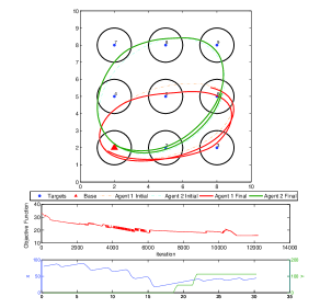
Figure 2: 8-targets, 2-agents, TPBVP trajectories (T=30) $J^{*}=15.82$

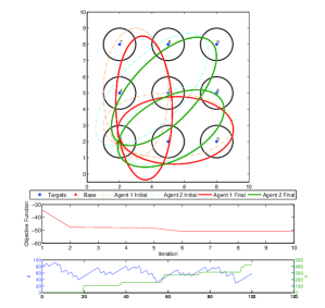
Figure 3: 8-targets, 2-agents, Elliptical trajectories (T=100) $J^{*}=-50.9$

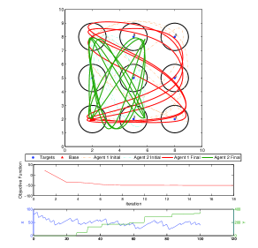
Figure 4: 8-targets, 2-agents, Fourier series trajectories (T=100) $J^{*}=-50.18$

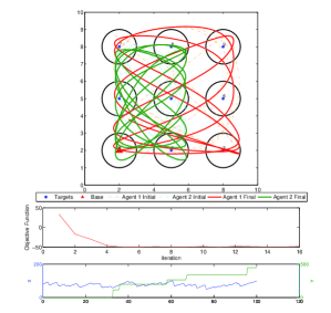
Figure 5: 8-targets, 2-agents, Random data processes - Fourier series trajectories $J^{*}=-48.05$

VI Conclusions

We have developed a new method for trajectory planning in the data harvesting problem. An optimal control formulation provides initial insights for the solution, but it is computationally intractable, especially in the case where the data generating processes are stochastic. We propose an agent trajectory parameterization in terms of general function families which are optimized on line through the use of IPA. Explicit results are provided for the case of elliptical and Fourier series trajectories. We have shown robustness of the solution with respect to stochastic data generation processes by considering stochastic data arrivals at targets. Natural next steps include constraining trajectories to urban setting obstacles in the mission space.

Appendix A Elliptical Trajectories

In order to calculate the IPA derivatives we need to have the derivative of state variable with respect to all the parameter vector $\Theta_{j}=[A_{j},B_{j},a_{j},b_{j},\phi_{j}]$ for all agents $j$. These derivatives do not depend on the events happening in the system since the trajectories of agents are fixed at each iteration. For now we assume $\mathcal{E}_{j}=1$ for all $j=1,\dots,N$ hence, we drop the superscript. We have:

$$\frac{\partial s^{x}_{j}}{\partial A_{j}}=1,\qquad\frac{\partial s^{x}_{j}}{\partial B_{j}}=0$$ (39)

$$\frac{\partial s^{x}_{j}}{\partial a_{j}}=\cos\rho_{j}(t)\cos\phi_{j},\qquad\frac{\partial s^{x}_{j}}{\partial b_{j}}=-\sin\rho_{j}(t)\sin\phi_{j}$$ (40)

$$\frac{\partial s^{x}_{j}}{\partial\phi_{j}}=-a_{j}\cos\rho_{j}(t)\sin\phi_{j}-b_{j}\sin\rho_{j}(t)\cos\phi_{j}$$ (41)

$$\frac{\partial s^{y}_{j}}{\partial A_{j}}=0,\qquad\frac{\partial s^{y}_{j}}{\partial B_{j}}=1$$ (42)

$$\frac{\partial s^{y}_{j}}{\partial a_{j}}=\cos\rho_{j}(t)\sin\phi_{j},\qquad\frac{\partial s^{y}_{j}}{\partial b_{j}}=\sin\rho_{j}(t)\cos\phi_{j}$$ (43)

$$\frac{\partial s^{y}_{j}}{\partial\phi_{j}}=a_{j}\cos\rho_{j}(t)\cos\phi_{j}-b_{j}\sin\rho_{j}(t)\sin\phi_{j}$$ (44)

Also the time derivative of the position state variables are calculated as below:

$$\dot{s}_{j}^{x}(t)=-a_{j}\dot{\rho}_{j}(t)\sin\rho_{j}(t)\cos\phi_{j}+b_{j}\dot{\rho}_{j}(t)\cos\rho_{j}(t)\sin\phi_{j}$$ (45)

$$\dot{s}_{j}^{y}(t)=-a_{j}\dot{\rho}_{j}(t)\sin\rho_{j}(t)\sin\phi_{j}+b_{j}\dot{\rho}_{j}(t)\cos\rho_{j}(t)\cos\phi_{j}$$ (46)

The gradient of the last term in the $J_{e}$ in (34) needs to be calculated separately. We have for $j\neq l$, $\frac{\partial\mathcal{C}_{j}}{\partial\Theta_{l}}=0$ and for $j=l$:

where

$$\begin{split}\frac{\partial f^{1}_{j}}{\partial A_{j}}&=-2\Big{(}\frac{w_{\!{}_{B}}^{x}-A_{j}}{a_{j}^{2}}\Big{)},\quad\frac{\partial f^{1}_{j}}{\partial B_{j}}=-2\Big{(}\frac{w_{\!{}_{B}}^{y}-B_{j}}{b_{j}^{2}}\Big{)}\\ \frac{\partial f^{1}_{j}}{\partial a_{j}}&=-2\Big{(}\frac{(w_{\!{}_{B}}^{x}-A_{j})^{2}}{a_{j}^{3}}\Big{)},\quad\frac{\partial f^{1}_{j}}{\partial b_{j}}=-2\Big{(}\frac{(w_{\!{}_{B}}^{y}-B_{j})^{2}}{b_{j}^{3}}\Big{)}\\ \end{split}$$

$$\begin{split}\frac{\partial f^{2}_{j}}{\partial A_{j}}&=-2\Big{(}\frac{w_{\!{}_{B}}^{x}-A_{j}}{b_{j}^{2}}\Big{)},~{}\frac{\partial f^{2}_{j}}{\partial B_{j}}=-2\Big{(}\frac{w_{\!{}_{B}}^{y}-B_{j}}{a_{j}^{2}}\Big{)}\\ \frac{\partial f^{2}_{j}}{\partial a_{j}}&=-2\Big{(}\frac{(w_{\!{}_{B}}^{y}-B_{j})^{2}}{a_{j}^{3}}\Big{)},~{}\frac{\partial f^{2}_{j}}{\partial b_{j}}=-2\Big{(}\frac{(w_{\!{}_{B}}^{x}-A_{j})^{2}}{b_{j}^{3}}\Big{)}\\ \end{split}$$

$$\begin{split}\frac{\partial f^{3}_{j}}{\partial A_{j}}&=-\Big{(}\frac{(b_{j}^{2}-a_{j}^{2})(w_{\!{}_{B}}^{y}-B_{j})}{a_{j}^{2}b_{j}^{2}}\Big{)}\\ \frac{\partial f^{3}_{j}}{\partial B_{j}}&=-\Big{(}\frac{(b_{j}^{2}-a_{j}^{2})(w_{\!{}_{B}}^{x}-A_{j})}{a_{j}^{2}b_{j}^{2}}\Big{)}\end{split}$$

$$\begin{split}\frac{\partial f^{3}_{j}}{\partial a_{j}}&=-2\Big{(}\frac{(w_{\!{}_{B}}^{x}-A_{j})(w_{\!{}_{B}}^{y}-B_{j})}{a_{j}^{3}}\Big{)}\\ \frac{\partial f^{3}_{j}}{\partial b_{j}}&=2\Big{(}\frac{(w_{\!{}_{B}}^{x}-A_{j})(w_{\!{}_{B}}^{y}-B_{j})}{b_{j}^{3}}\Big{)}\end{split}$$

Appendix B Fourier Series Trajectories

We calculate the position of agent $j$’s derivative with respect to all the Fourier parameters. The parameter vector is $\Theta_{j}=[f_{j}^{x},a_{0,j},\ldots,a_{\Gamma_{j}^{x}},b_{0,j},\ldots,b_{\Gamma_{j}^{y}},\phi_{1,j},\ldots,\phi_{\Gamma_{j}^{x}},\xi_{1,j},\ldots,\xi_{\Gamma_{j}^{y}}]$. So we have:

$$\frac{\partial s^{x}_{j}}{\partial a_{0,j}}=1,\qquad\frac{\partial s^{x}_{j}}{\partial b_{0,j}}=0$$ (47)

$$\frac{\partial s^{x}_{j}}{\partial a_{n,j}}=\sin(2\pi nf_{j}^{x}\rho_{j}(t)+\phi^{x}_{n,j}),\qquad\frac{\partial s^{x}_{j}}{\partial b_{n,j}}=0$$ (48)

$$\frac{\partial s^{x}_{j}}{\partial\phi^{x}_{n,j}}=a_{n,j}\cos(2\pi nf_{j}^{x}\rho_{j}(t)+\phi^{x}_{n,j})\qquad\frac{\partial s^{x}_{j}}{\partial\phi^{y}_{n,j}}=0$$ (49)

$$\frac{\partial s^{x}_{j}}{\partial f_{j}^{x}}=2\pi\rho_{j}(t)\displaystyle\sum_{n=1}^{\Gamma_{j}^{x}}a_{n,j}n\cos(2\pi nf_{j}^{x}\rho_{j}(t)+\phi^{x}_{n,j}),$$ (50)

$$\frac{\partial s^{y}_{j}}{\partial b_{0,j}}=1,\qquad\frac{\partial s^{y}_{j}}{\partial a_{0,j}}=0$$ (51)

$$\frac{\partial s^{y}_{j}}{\partial b_{n,j}}=\sin(2\pi nf_{j}^{y}\rho_{j}(t)+\phi^{y}_{n,j}),\qquad\frac{\partial s^{y}_{j}}{\partial a_{n,j}}=0$$ (52)

$$\frac{\partial s^{y}_{j}}{\partial\phi^{y}_{n,j}}=b_{n,j}\cos(2\pi nf_{j}^{y}\rho_{j}(t)+\phi^{y}_{n,j})\qquad\frac{\partial s^{y}_{j}}{\partial\phi^{x}_{n,j}}=0$$ (53)

$$\frac{\partial s^{y}_{j}}{\partial f_{j}^{x}}=0$$ (54)

Also the time derivative of the position state variables are calculated as below:

$$\dot{s}_{j}^{x}(t)=\dot{\rho}_{j}(t)\sum_{n=1}^{\Gamma_{j}^{x}}2\pi nf_{j}^{x}a_{n,j}\cos(2\pi nf_{j}^{x}\rho_{j}(t)+\phi^{x}_{n,j}),$$ (55)

$$\dot{s}_{j}^{y}(t)=\dot{\rho}_{j}(t)\sum_{n=1}^{\Gamma_{j}^{y}}2\pi nf_{j}^{y}a_{n,j}\cos(2\pi nf_{j}^{y}\rho_{j}(t)+\phi^{x}_{n,j}),$$ (56)

Appendix C IPA events and derivatives

In this section, we derive all event time derivatives and state derivatives with respect to the controllable parameter $\Theta$ for each event by applying the IPA equations.

1. Event $\xi_{i}^{0}$: This event causes a transition from $X_{i}(t)>0$, $t<\tau_{k}$ to $X_{i}(t)=0$, $t\geq\tau_{k}$. The switching function is $g_{k}(\Theta,{\bf X})=X_{i}$ so $\frac{\partial g_{k}}{\partial X_{i}}=1$. From (25) and (4):

$$\begin{split}{\tau_{k}^{{}^{\prime}}}&=-\Big{(}\frac{\partial g_{k}}{\partial X_{i}}f_{k}(\tau_{k}^{-})\Big{)}^{-1}\Big{(}\frac{\partial g_{k}}{\partial\Theta}+\frac{\partial g_{k}}{\partial X_{i}}{X_{i}^{\prime}(\tau_{k}^{-})}\Big{)}\\ &=-\frac{X_{i}^{\prime}(\tau_{k}^{-})}{\sigma_{i}(\tau_{k})-\mu_{ij}P_{ij}(\tau_{k})}\end{split}$$ (57)

where agent $j$ is the one connected to $i$ at $t=\tau_{k}$ and we have used the assumption that two events occur at the same time w.p. $0$, hence $\sigma_{i}(\tau_{k}^{-})=\sigma_{i}(\tau_{k})$. From (26)-(27), since $\dot{X}_{i}(t)=0$, for $\tau_{k}\leq t<\tau_{k+1}$:

$$\frac{d}{dt}X_{i}^{\prime}(t)=\frac{\partial\dot{X}_{i}(t)}{\partial X_{i}(t)}X_{i}^{\prime}(t)+{\dot{X}_{i}^{\prime}(t)}=0$$ (58)

$$\begin{split}&X_{i}^{\prime}(\tau_{k}^{+})=X_{i}^{\prime}(\tau_{k}^{-})+\Big{[}\Big{(}\sigma_{i}(\tau_{k})-\mu_{ij}P_{ij}(\tau_{k})\Big{)}-0\Big{]}{\tau_{k}}^{\prime}\\ &=X_{i}^{\prime}(\tau_{k}^{-})-\frac{X_{i}^{\prime}(\tau_{k}^{-})\Big{(}\sigma_{i}(\tau_{k})-\mu_{ij}P_{ij}(\tau_{k})\Big{)}}{\sigma_{i}(\tau_{k})-\mu_{ij}P_{ij}(\tau_{k})}=0\end{split}$$ (59)

For $X_{r}(t)$, $r\neq i$, the dynamics of $X_{r}(t)$ in (4) are unaffected and we have:

$$X_{r}^{\prime}(\tau_{k}^{+})=X_{r}^{\prime}(\tau_{k}^{-})$$ (60)

If $X_{r}(\tau_{k})>0$ and agent $l$ is connected to it, then

$$\begin{split}&\frac{d}{dt}X_{r}^{\prime}(t)=\frac{\partial\dot{X}_{r}(t)}{\partial X_{r}(t)}X_{r}^{\prime}(t)+{\dot{X}_{r}^{\prime}(t)}\\ &=\frac{\partial}{\partial\Theta}\Big{(}\sigma_{r}(t)-\mu_{rl}P_{rl}(\tau_{k})\Big{)}=-\mu_{rl}P_{rl}^{\prime}(t)\end{split}$$ (61)

and if ${X}_{r}(t)=0$ in $[\tau_{k},\tau_{k+1}]$ or if no agents are connected to $i$, then and $\frac{d}{dt}X_{r}^{\prime}(t)=0$.
For $Y_{r}(t)$, $r=1,\dots,M$, the dynamics of $Y_{r}(t)$ in (7) are not affected by the event $\xi_{i}^{0}$ at $\tau_{k}$, hence

$$Y_{r}^{\prime}(\tau_{k}^{+})=Y_{r}^{\prime}(\tau_{k}^{-})$$ (62)

and since $\dot{Y}_{r}(t)=\beta_{r}(t)$, for $\tau_{k}\leq t<\tau_{k+1}$:

$$\frac{d}{dt}Y_{r}^{\prime}(t)=\frac{\partial\dot{Y}_{r}(t)}{\partial Y_{r}(t)}Y_{r}^{\prime}(t)+{\dot{Y}_{r}^{\prime}(t)}=\beta_{r}^{\prime}(t)$$ (63)

For $Z_{ij}(t)$, we must have $Z_{ij}(\tau_{k})>0$ since $X_{i}(\tau_{k}^{-})>0$, hence $\tilde{\mu}_{ij}(\tau_{k}^{-})>0$ and from (27):

$$\begin{split}&Z_{ij}^{\prime}(\tau_{k}^{+})=Z_{ij}^{\prime}(\tau_{k}^{-})+\Big{[}\dot{Z}_{ij}(\tau_{k}^{-})-\dot{Z}_{ij}(\tau_{k}^{+})\Big{]}\tau_{k}^{\prime}\\ &=Z_{ij}^{\prime}(\tau_{k}^{-})+\Big{[}\tilde{\mu}_{ij}(\tau_{k}^{-})-\tilde{\mu}_{ij}(\tau_{k}^{+})\Big{]}P_{ij}(\tau_{k})\tau_{k}^{\prime}\end{split}$$ (64)

Since $X_{i}(\tau_{k}^{-})>0$, from (5) we have $\tilde{\mu}_{ij}(\tau_{k}^{-})=\mu_{ij}$. At $\tau_{k}^{+}$, $j$ remains connected to target $i$ with $\tilde{\mu}_{ij}(\tau_{k}^{+})=\sigma_{i}(\tau_{k}^{+})/P_{ij}(\tau_{k})=\sigma_{i}(\tau_{k})/P_{ij}(\tau_{k})$ and we get

$$\begin{split}Z_{ij}^{\prime}(\tau_{k}^{+})&=Z_{ij}^{\prime}(\tau_{k}^{-})+\frac{-X_{i}^{\prime}(\tau_{k}^{-})\Big{[}\mu_{ij}P_{ij}(\tau_{k})-\sigma_{i}(\tau_{k})\Big{]}}{\sigma_{i}(\tau_{k})-\mu_{ij}P_{ij}(\tau_{k})}\\ &=Z_{ij}^{\prime}(\tau_{k}^{-})+X_{i}^{\prime}(\tau_{k}^{-})\end{split}$$ (65)

From (26) for $\tau_{k}\leq t<\tau_{k+1}$:

$$\begin{split}&\frac{d}{dt}Z_{ij}^{\prime}(t)=\frac{\partial\dot{Z}_{ij}(t)}{\partial Z_{ij}(t)}Z_{ij}^{\prime}(t)+\frac{\partial{\dot{Z}_{ij}(t)}}{\partial\Theta}\\ &=\frac{\partial{\dot{Z}_{ij}(t)}}{\partial\Theta}=\frac{\partial}{\partial\Theta}\Big{(}\tilde{\mu}_{ij}(t)P_{ij}(t)-\beta_{ij}P_{\!{}_{Bj}}(t)\Big{)}\end{split}$$ (66)

Since $\tilde{\mu}_{ij}(t)=\sigma_{i}(t)/P_{ij}(t)$ for the agent which remains connected to target $i$ after this event, it follows that $\frac{\partial}{\partial\Theta}[\tilde{\mu}_{ij}(t)P_{ij}(t)]=0$. Moreover, $P_{\!{}_{Bj}}(t)=0$ by our assumption that agents cannot be within range of the base and targets at the same time and we get

$$\frac{d}{dt}Z_{ij}^{\prime}(t)=0$$ (67)

Otherwise, for $r\neq j$, we have $\tilde{\mu}_{ir}(t)=0$ and we get:

$$\frac{d}{dt}Z_{ir}^{\prime}(t)=-\beta_{ir}P_{\!{}_{Br}}^{\prime}(t)$$ (68)

Finally, for $Z_{rj}(t)$, $r\neq i$ we have $Z_{rj}^{\prime}(\tau_{k}^{+})=Z_{rj}^{\prime}(\tau_{k}^{-})$. If $Z_{rj}(t)=0$ in $[\tau_{k},\tau_{k+1})$, then $\frac{d}{dt}Z_{rj}^{\prime}(t)=0$. Otherwise, we get $\frac{d}{dt}Z_{rj}^{\prime}(t)$ from (66) with $i$ replaced by $r$.

2. Event $\xi_{i}^{+}$: This event causes a transition from $X_{i}(t)=0$, $t\leq\tau_{k}$ to $X_{i}(t)>0$, $t>\tau_{k}$. Note that this transition can occur as an exogenous event when an empty queue $X_{i}(t)$ gets a new arrival in which case we simply have $\tau_{k}^{\prime}=0$ since the exogenous event is independent of the controllable parameters. In the endogenous case, however, we have the switching function $g_{k}(\Theta,{\bf X})=\sigma_{i}(t)-\mu_{ij}P_{ij}(t)$ in which agent $j$ is connected to target $i$ at $t=\tau_{k}$. Assuming $\frac{\partial s_{j}}{\partial\Theta}=\big{[}\frac{\partial s_{j}^{x}}{\partial\Theta}~{}\frac{\partial s_{j}^{y}}{\partial\Theta}\big{]}^{\top}$ and $\dot{s}_{j}=[\dot{s}_{j}^{x}~{}\dot{s}_{j}^{y}]^{\top}$, from (25):

$$\begin{split}{\tau_{k}}^{\prime}&=-\Big{(}\frac{\partial g_{k}}{\partial s_{j}}\frac{\partial s_{j}}{\partial\Theta}\Big{)}\Big{(}{\frac{\partial g_{k}}{\partial s_{j}}\dot{s}_{j}(\tau_{k})}\Big{)}^{-1}\end{split}$$ (69)

At $\tau_{k}$ we have $\sigma_{i}(\tau_{k})=\mu_{ij}P_{ij}(\tau_{k})$. Therefore from (27):

$$\begin{split}&X_{i}^{\prime}(\tau_{k}^{+})=X_{i}^{\prime}(\tau_{k}^{-})+[\dot{X}_{i}(\tau_{k}^{-})-\dot{X}_{i}(\tau_{k}^{+})]{\tau_{k}}^{\prime}\\ &=X_{i}^{\prime}(\tau_{k}^{-})+\Big{(}0-\sigma_{i}(\tau_{k})+\mu_{ij}P_{ij}(\tau_{k})\Big{)}{\tau_{k}}^{\prime}=X_{i}^{\prime}(\tau_{k}^{-})\end{split}$$ (70)

Having $X_{i}(t)>0$ in $[\tau_{k},\tau_{k+1})$ we know $\dot{X}_{i}(t)=\sigma_{i}(t)-\mu_{ij}P_{ij}(t)$ therefor, we can get $\frac{d}{dt}X_{i}^{\prime}(t)$ from (61) with $r$ and $l$ replaced by $i$ and $j$. For $X_{r}(t)$, $r\neq i$, if $X_{r}(\tau_{k})>0$ and agent $l$ is connected to $r$ then $\dot{X}_{r}(\tau_{k})=\sigma_{r}(\tau_{k})-\mu_{rl}P_{rl}(\tau_{k})$, therefor, we get $X^{\prime}_{r}(\tau_{k}^{+})$ from (60) while in $[\tau_{k},\tau_{k+1})$ we have $\frac{d}{dt}X^{\prime}_{r}(t)$ from (61). If $X_{r}(\tau_{k})=0$ or if no agent is connected to target $r$, $\dot{X}_{r}(\tau_{k})=0$. Thus, $X^{\prime}_{r}(\tau_{k}^{+})=X^{\prime}_{r}(\tau_{k}^{-})$ and $\frac{d}{dt}X^{\prime}_{r}(t)=0$.
For $Y_{r}(t)$, $r=1,\dots,M$ the dynamics of $Y_{r}(t)$ in (7) are not affected by the event at $\tau_{k}$ hence, we can get $Y^{\prime}_{r}(\tau_{k}^{+})$ and $\frac{d}{dt}Y^{\prime}_{r}(t)$ in $[\tau_{k},\tau_{k+1})$ from (62) and (63) respectively.
For $Z_{ij}(t)$ assuming agent $j$ is the one connected to target $i$, we have:

$$\begin{split}&Z^{\prime}_{ij}(\tau_{k}^{+})=Z^{\prime}_{ij}(\tau_{k}^{-})+\Big{[}\dot{Z}_{ij}(\tau_{k}^{-})-\dot{Z}_{ij}(\tau_{k}^{+})\Big{]}\tau^{\prime}_{k}\\ &=Z^{\prime}_{ij}(\tau_{k}^{-})+\Big{[}\tilde{\mu}_{ij}(\tau_{k}^{-})-\tilde{\mu}_{ij}(\tau_{k}^{+})\Big{]}P_{ij}(\tau_{k})\tau^{\prime}_{k}=Z^{\prime}_{ij}(\tau_{k}^{-})\end{split}$$ (71)

In the above equation, $\tilde{\mu}_{ij}(\tau_{k}^{+})=\mu_{ij}$ because $X_{i}(\tau_{k}^{+})>0$. Also, $\mu_{ij}P_{ij}(\tau_{k})=\sigma_{i}(\tau_{k})$ and $\tilde{\mu}_{ij}(\tau_{k}^{-})=\frac{\sigma_{i}(\tau_{k})}{P_{ij}(\tau_{k})}$ results in $\tilde{\mu}_{ij}(\tau_{k}^{+})=\mu_{ij}$. For $Z_{il}(t)$, $l\neq j$ , agent $l$ cannot be connected to target $i$ at $\tau_{k}$ so we have, $Z^{\prime}_{il}(\tau_{k}^{+})=Z^{\prime}_{il}(\tau_{k}^{-})$ and $\frac{d}{dt}Z^{\prime}_{il}(t)=0$ in $[\tau_{k},\tau_{k+1})$. For $Z_{rl}(t)$ ,$r\neq i$ and $l\neq j$ using the assumption that two events occur at the same time w.p. 0, the dynamics of $Z_{rl}(t)$ are not affected at $\tau_{k}$, hence we get $\frac{d}{dt}Z^{\prime}_{rl}(t)$ from (66) for $i$ and $j$ replaced by $r$ and $l$.

3. Event $\zeta_{ij}^{0}$: This event causes a transition from $Z_{ij}(t)>0$ for $t<\tau_{k}$ to $Z_{ij}(t)=0$ for $t\geq\tau_{k}$. The switching function is $g_{k}(\Theta,{\bf X})=Z_{ij}(t)$ so $\frac{\partial g_{k}}{\partial Z_{ij}}=1$. From (25):

$$\begin{split}&{\tau_{k}}^{\prime}=-\Big{(}\frac{\partial g_{k}}{\partial Z_{ij}}f_{k}(\tau^{-}_{k})\Big{)}^{-1}\Big{(}\frac{\partial g_{k}}{\partial\Theta}+\frac{\partial g_{k}}{\partial Z_{ij}}{Z_{ij}^{\prime}(\tau^{-}_{k})}\Big{)}\\ &=-\frac{Z_{ij}^{\prime}(\tau^{-}_{k})}{\tilde{\mu}_{ij}(\tau^{-}_{k})P_{ij}(\tau^{-}_{k})-\beta_{ij}P_{\!{}_{Bj}}(\tau^{-}_{k})}=\frac{Z_{ij}^{\prime}(\tau^{-}_{k})}{\beta_{ij}P_{\!{}_{Bj}}(\tau_{k})}\end{split}$$ (72)

Since $Z_{ij}(t)$ is being emptied at $\tau_{k}$, by the assumption that agents can not be in range with the base and targets at the same time, we have $P_{ij}(\tau_{k})=0$. Then from (27):

$$\begin{split}&Z^{\prime}_{ij}(\tau_{k}^{+})=Z^{\prime}_{ij}(\tau_{k}^{-})+\Big{[}-\beta_{ij}P_{\!{}_{Bj}}(\tau_{k})-0\Big{]}{\tau_{k}}^{\prime}\\ &=Z^{\prime}_{ij}(\tau_{k}^{-})-\Big{[}\beta_{ij}P_{\!{}_{Bj}}(\tau_{k})\Big{]}\frac{Z_{ij}^{\prime}(\tau^{-}_{k})}{\beta_{ij}P_{\!{}_{Bj}}(\tau_{k})}=0\end{split}$$ (73)

Since $\dot{Z}_{ij}(t)=0$ in $[\tau_{k},\tau_{k+1})$:

$$\frac{d}{dt}Z^{\prime}_{ij}(t)=\frac{\partial\dot{Z}_{ij}(t)}{\partial Z_{ij}(t)}Z^{\prime}_{ij}(t)+\frac{\partial{\dot{Z}_{ij}(t)}}{\partial\Theta}=0$$ (74)

For $Z_{rl}(t)$, $r\neq i$ or $l\neq j$, the dynamics in (6) are not affected at $\tau_{k}$, hence:

$$Z^{\prime}_{rl}(\tau_{k}^{+})=Z^{\prime}_{rl}(\tau_{k}^{-})$$ (75)

if $Z_{rl}(\tau_{k})>0$, the value for $\frac{d}{dt}Z^{\prime}_{rl}(t)$ is calculated by (66) with $r$ and $l$ replacing $i$ and $j$ respectively. If $Z_{rl}(\tau_{k})=0$ then $\frac{d}{dt}Z^{\prime}_{rl}(t)=0$.
For $Y_{i}(t)$ we have $\beta_{i}(\tau_{k}^{+})=0$ since the agent has emptied its queue, hence:

$$\begin{split}&Y^{\prime}_{i}(\tau_{k}^{+})=Y^{\prime}_{i}(\tau_{k}^{-})+\Big{[}\dot{Y}_{i}(\tau_{k}^{-})-\dot{Y}_{i}(\tau_{k}^{+})\Big{]}\tau^{\prime}_{k}\\ &=Y^{\prime}_{i}(\tau_{k}^{-})+[\beta_{ij}P_{\!{}_{Bj}}(\tau_{k})-0]\frac{Z_{ij}^{\prime}(\tau^{-}_{k})}{\beta_{ij}P_{\!{}_{Bj}}(\tau_{k})}\\ &=Y^{\prime}_{i}(\tau_{k}^{-})+Z_{ij}^{\prime}(\tau^{-}_{k})\end{split}$$ (76)

In $[\tau_{k},\tau_{k+1})$ we can get $\frac{d}{dt}Y^{\prime}_{i}(t)=0$. For $Y_{r}(t)$, $r\neq i$ the dynamics of $Y_{r}(t)$ in (7) are not affected by the event at $\tau_{k}$ hence, $Y^{\prime}_{r}(\tau_{k}^{+})$ and $\frac{d}{dt}Y^{\prime}_{r}(t)$ in $[\tau_{k},\tau_{k+1})$ are calculated from (62) and (63) respectively. The dynamics of $X_{r}(t)$, $r=1,\dots,M$ is are not affected at $\tau_{k}$ since the event at $\tau_{k}$ is happening at the base. We have $X_{r}^{\prime}(\tau_{k}^{+})=X_{r}^{\prime}(\tau_{k}^{-})$. If $X_{r}(\tau_{k})>0$ then we have $\frac{d}{dt}X^{\prime}_{r}(t)$ from (61) and if $X_{r}(\tau_{k})=0$ then $\frac{d}{dt}X^{\prime}_{r}(t)=0$ in $[\tau_{k},\tau_{k+1})$.

4. Event $\delta_{ij}^{+}$: This event causes a transition from $D^{+}_{ij}(t)=0$ for $t\leq\tau_{k}$ to $D^{+}_{ij}(t)>0$ for to $t>\tau_{k}$. It is the moment that agent $j$ leaves target $i$’s range. The switching function is $g_{k}(\Theta,{\bf X})=D_{ij}(t)-r_{ij}$ , from (25):

$${\tau_{k}}^{\prime}=-\frac{\partial D_{ij}}{\partial s_{j}}\frac{\partial s_{j}}{\partial\Theta}\Big{(}\frac{\partial D_{ij}}{\partial s_{j}}\dot{s}_{j}(\tau_{k})\Big{)}^{-1}$$ (77)

If agent $j$ was connected to target $i$ at $\tau_{k}$ then by leaving the target, it is possible that another agent $l$ which is within range with target $i$ connects to that target. This means $\dot{X}_{i}(\tau_{k}^{+})=\sigma_{i}(\tau_{k})-\mu_{il}P_{il}(\tau_{k})$ and $\dot{X}_{i}(\tau_{k}^{-})=\sigma_{i}(\tau_{k})-\mu_{ij}P_{ij}(\tau_{k})$, with $P_{ij}(\tau_{k})=0$, from (27) we have

$$X_{i}^{\prime}(\tau_{k}^{+})=X_{i}^{\prime}(\tau_{k}^{-})-\mu_{il}P_{il}(\tau_{k})\tau_{k}^{\prime}$$ (78)

If $X_{i}(\tau_{k})>0$, $\frac{d}{dt}X^{\prime}_{i}(t)$ in $[\tau_{k},\tau_{k+1})$ is as in (61) with $r$ replaced by $i$ and if $X_{i}(\tau_{k})=0$ then $\frac{d}{dt}X^{\prime}_{i}(t)=0$. On the other hand, if agent $j$ was not connected to target $i$ at $\tau_{k}$, we know that some $l\neq j$ is already connected to target $i$. This means agent $j$ leaving target $i$ cannot affect the dynamics of $X_{i}(t)$ so we have $X_{i}^{\prime}(\tau_{k}^{+})=X_{i}^{\prime}(\tau_{k}^{-})$ and $\frac{d}{dt}X_{i}^{\prime}(t)$ is calculated from (61) with $r$ replaced by $i$.
For $X_{r}(t)$, $r\neq i$ the dynamics in (4) are not affected by the event at $\tau_{k}$ hence, we get $X_{r}^{\prime}(\tau_{k}^{+})$ from (60). If $X_{r}(\tau_{k})>0$ the time derivative $\frac{d}{dt}X^{\prime}_{r}(t)$ in $[\tau_{k},\tau_{k+1})$ can be calculated from (61) and if $X_{r}(\tau_{k})=0$ then $\frac{d}{dt}X^{\prime}_{r}(t)=0$.
For $Y_{r}(t)$, $r=1,\ldots,,M$, the dynamics in (7) are not also affected by the event at $\tau_{k}$ hence, we get $Y_{r}(\tau_{k}^{+})$ from (62) and in $[\tau_{k},\tau_{k+1})$ the $\frac{d}{dt}Y^{\prime}_{r}(t)$ is calculated from (63).
For $Z_{ij}(t)$, the dynamics in (6) are not affect at $\tau_{k}$, regardless of the fact that agent $j$ is connected to target $i$ or not. We have $\dot{Z}_{ij}(\tau_{k}^{-})=\tilde{\mu}_{ij}(\tau_{k})P_{ij}(\tau_{k})$ with $P_{ij}(\tau_{k})=0$ and $\dot{Z}_{ij}(\tau_{k}^{+})=0$, hence from (27):

$$\begin{split}&Z^{\prime}_{ij}(\tau_{k}^{+})=Z^{\prime}_{ij}(\tau_{k}^{-})+\Big{[}\dot{Z}_{ij}(\tau_{k}^{-})-\dot{Z}_{ij}(\tau_{k}^{+})\Big{]}\tau^{\prime}_{k}\\ &=Z^{\prime}_{ij}(\tau_{k}^{-})+\tilde{\mu}_{ij}(\tau_{k})P_{ij}(\tau_{k})\tau^{\prime}_{k}=Z^{\prime}_{ij}(\tau_{k}^{-})\end{split}$$ (79)

and in $[\tau_{k},\tau_{k+1})$ , we have $\frac{d}{dt}Z^{\prime}_{ij}(t)=0$ using (66) knowing $P_{ij}(\tau_{k})=P_{\!{}_{Bj}}(\tau_{k})=0$. For $Z_{rl}(t)$, $r\neq i$ or $l\neq j$, the dynamics of $Z_{rl}(t)$ are not affected at $\tau_{k}$ hence (75) holds and in $[\tau_{k},\tau_{k+1})$ again we can use (66) with $i$ and $j$ replaced by $r$ and $l$.

5. Event $\delta_{ij}^{0}$: This event causes a transition from $D^{+}_{ij}(t)>0$ for $t<\tau_{k}$ to $D^{+}_{ij}(t)=0$ for to $t\geq\tau_{k}$. The event is the moment that agent $j$ enters target $i$’s range. The switching function is $g_{k}(\Theta,{\bf X})=D_{ij}(t)-r_{ij}$. From (25) we can get ${\tau_{k}}^{\prime}$ from (77). If no other agent is already connected to target $i$, agent $j$ connects to it. Otherwise, if another agent is already connected to target $i$, no connection is established. For $X_{i}(t)$, the dynamics in (4) are not affected in both cases, hence, (70) holds. If $X_{i}(t)>0$ in $[\tau_{k},\tau_{k+1})$ we calculate $\frac{d}{dt}X^{\prime}_{i}(t)$ using (61) with $l$ being the appropriate connected agent to target $i$. If $X_{i}(\tau_{k}^{-})=0$, $\frac{d}{dt}X^{\prime}_{i}(t)=0$. For $X_{r}(t)$, $r\neq i$ the dynamics in (4) are not affected by the event at $\tau_{k}$. Hence, we get $X_{r}^{\prime}(\tau_{k}^{+})$ from (60). If $X_{r}(\tau_{k})>0$ we calculate $\frac{d}{dt}X^{\prime}_{r}(t)$ from (61) with $i$ replaced by $r$ and if $X_{r}(\tau_{k})=0$ then $\frac{d}{dt}X^{\prime}_{r}(t)=0$.
For $Y_{r}(t)$, $r=1,\dots,M$ again the dynamics in (7) are not affected at $tau_{k}$ so both (62) and (63) hold.
For $Z_{ij}(t)$, with agent $j$ being connected or not to target $i$ at $\tau_{k}$ the dynamics of $Z_{ij}(t)$ are unaffected at $\tau_{k}$, hence (75) holds for $i$ and $j$ and in $[\tau_{k},\tau_{k+1})$ the $\frac{d}{dt}Z^{\prime}_{ij}(t)$ is calculated through (66). For $Z_{rl}(t)$, $r\neq i$ or $l\neq j$ the dynamics are unaffected (75) holds again. In $[\tau_{k},\tau_{k+1})$, $\frac{d}{dt}Z^{\prime}_{rl}(t)$ is given through (66) with $i$ and $j$ replaced by $r$ and $l$.

6. Event $\Delta_{j}^{+}$: This event causes a transition from $D^{+}_{\!{Bj}}(t)=0$ for $t\leq\tau_{k}$ to $D^{+}_{\!{Bj}}(t)\geq 0$ for $t>\tau_{k}$. The switching function is $g_{k}(\Theta,{\bf X})=D_{\!{}_{Bj}}(t)-r_{\!{}_{Bj}}$.

$${\tau_{k}}^{\prime}=-\frac{\partial D{\!{}_{Bj}}}{\partial s_{j}}\frac{\partial s_{j}}{\partial\Theta}\Big{(}\frac{\partial D_{\!{}_{Bj}}}{\partial s_{j}}\dot{s}_{j}(\tau_{k})\Big{)}^{-1}$$ (80)

Similar to the previous event, the dynamics of $X_{i}(t)$ are unaffected at $\tau_{k}$ hence, we have $X_{i}^{\prime}(\tau_{k}^{+})$ calculated from (70). If $X_{i}(t)>0$ in $[\tau_{k},\tau_{k+1})$ we calculate $\frac{d}{dt}X^{\prime}_{i}(t)$ through (61) and if $X_{i}(\tau_{k}^{-})=0$, $\frac{d}{dt}X^{\prime}_{i}(t)=0$.
For $Y_{r}(t)$, $r=1,\ldots,,M$, the dynamics of $Y_{r}(t)$ in (7) are not affected at $\tau_{k}$, hence, we get $Y_{r}(\tau_{k}^{+})$ from (62) and in $[\tau_{k},\tau_{k+1})$, $\frac{d}{dt}Y^{\prime}_{r}(t)$ is calculated from (63).
For $Z_{ij}(t)$, Using the fact that agent $j$ can only be connected to one target or the base, we have $\dot{Z}_{ij}(\tau_{k}^{-})=\beta_{ij}(\tau_{k})P_{\!{}_{Bj}}(\tau_{k})$ with $P_{\!{}_{Bj}}(\tau_{k})=0$ and $\dot{Z}_{ij}(\tau_{k}^{+})=0$, hence (75) holds with $i$ and $j$ replacing $r$ and $l$. In $[\tau_{k},\tau_{k+1})$ from (26):

$$\begin{split}&\frac{d}{dt}Z^{\prime}_{ij}(t)=\frac{\partial\dot{Z}_{ij}(t)}{\partial Z_{ij}(t)}Z^{\prime}_{ij}(t)+\frac{\partial{\dot{Z}_{ij}(t)}}{\partial\Theta}\\ &=\frac{\partial{\dot{Z}_{ij}(t)}}{\partial\Theta}=-\beta_{ij}P^{\prime}_{\!{}_{Bj}}(t)\end{split}$$ (81)

As for $Z_{rl}(t)$, $r\neq i$ or $l\neq j$ the dynamics are unaffected so (75) holds. In $[\tau_{k},\tau_{k+1})$ we can calculate $\frac{d}{dt}Z^{\prime}_{rl}(t)$ through (66) with $j$ replacing $l$.

7. Event $\Delta_{j}^{0}$: This event causes a transition from $D^{+}_{\!{Bj}}(t)>0$ for $t<\tau_{k}$ to $D^{+}_{\!{Bj}}(t)=0$ for $t\geq\tau_{k}$. The switching function is $g_{k}(\Theta,{\bf X})=D_{\!{}_{Bj}}(t)-r_{\!{}_{Bj}}$. Using (25) we can get ${\tau_{k}}^{\prime}$ from (80). Similar with the previous event we have $X_{i}^{\prime}(\tau_{k}^{+})$ from (70). If $X_{i}(t)>0$ we can get $\frac{d}{dt}X^{\prime}_{i}(t)$ from (61) and if $X_{i}(\tau_{k}^{-})=0$ then $\frac{d}{dt}X^{\prime}_{i}(t)=0$.
For $Y_{r}(t)$, $r=1,\ldots,,M$, we again follow the previous event analysis so (62) and (63) hold.
For $Z_{ij}(t)$, the analysis is similar to event $\Delta_{j}^{+}$ so we can calculate $Z_{ij}^{\prime}(\tau_{k}^{+})$ and $\frac{d}{dt}Z^{\prime}_{ij}(t)$ in $[\tau_{k},\tau_{k+1})$ from (71) and (66) respectively. Also for $Z_{rl}(t)$, $r\neq i$ or $l\neq j$, (75) holds with same reasoning as previous event. In $[\tau_{k},\tau_{k+1})$ we calculate $\frac{d}{dt}Z^{\prime}_{rl}(t)$ from (66).

References

- [1] P. Corke, T. Wark, R. Jurdak, W. Hu, P. Valencia, and D. Moore, “Environmental wireless sensor networks,” in Proc. of the IEEE, vol. 98, pp. 1903–1917, 2010.
- [2] R. N. Smith, M. Schwager, S. L. Smith, D. Rus, and G. S. Sukhatme, “Persistent ocean monitoring with underwater gliders: Towards accurate reconstruction of dynamic ocean processes,” in Proc. - IEEE Int. Conf. on Robotics and Automation, pp. 1517–1524, 2011.
- [3] Z. Tang and U. Özgüner, “Motion planning for multitarget surveillance with mobile sensor agents,” IEEE Trans. on Robotics, vol. 21, pp. 898–908, 2005.
- [4] M. Zhong and C. G. Cassandras, “Distributed coverage contorol and data collection with mobile sensor networks,” IEEE Trans. on Automatic Cont.,, vol. 56, no. 10, pp. 2445–2455, 2011.
- [5] K. Chakrabarty, S. S. Iyengar, H. Qi, and E. Cho, “Grid coverage for surveillance and target location in distributed sensor networks,” IEEE Trans. on Computers, vol. 51, no. 12, pp. 1448–1453, 2002.
- [6] M. Cardei, M. T. Thai, Y. Li, and W. Wu, “Energy-efficient target coverage in wireless sensor networks,” 24th Annual INFOCOM 2005., pp. 1976–1984, 2005.
- [7] S. Alamdari, E. Fata, and S. L. Smith, “Persistent monitoring in discrete environments: Minimizing the maximum weighted latency between observations,” The Int. J. of Robotics Research, 2013.
- [8] C. G. Cassandras, X. Lin, and X. Ding, “An optimal control approach to the multi-agent persistent monitoring problem,” IEEE Trans. on Aut. Cont., vol. 58, pp. 947–961, April 2013.
- [9] D. Panagou, M. Turpin, and V. Kumar, “Decentralized goal assignment and trajectory generation in multi-robot networks,” CoRR, vol. abs/1402.3735, 2014.
- [10] A. T. Klesh, P. T. Kabamba, and A. R. Girard, “Path planning for cooperative time-optimal information collection,” Proc. of the American Cont. Conf., pp. 1991–1996, 2008.
- [11] J. L. Ny, M. a. Dahleh, E. Feron, and E. Frazzoli, “Continuous path planning for a data harvesting mobile server,” Proc. of the IEEE Conf. on Decision and Cont., pp. 1489–1494, 2008.
- [12] R. Moazzez-Estanjini and I. C. Paschalidis, “On delay-minimized data harvesting with mobile elements in wireless sensor networks,” Ad Hoc Networks, vol. 10, pp. 1191–1203, 2012.
- [13] M. Roscia, M. Longo, and G. Lazaroiu, “Smart City by multi-agent systems,” 2013 Int. Conf. on Renewable Energy Research and Applications IEEE, no. October, pp. 20–23, 2013.
- [14] K. Akkaya and M. Younis, “A survey on routing protocols for wireless sensor networks,” Ad Hoc Networks, vol. 3, pp. 325–349, 2005.
- [15] M. Liu, Y. Yang, and Z. Qin, “A survey of routing protocols and simulations in delay-tolerant networks,” Lecture Notes in Computer Science, vol. 6843 LNCS, pp. 243–253, 2011.
- [16] C. Chang, G. Yu, T. Wang, and C. Lin, “Path Construction and Visit Scheduling for Targets using Data Mules,” IEEE Trans. on Sys, Man, and Cybernetics: Systems, vol. 44, no. 10, pp. 1289–1300, 2014.
- [17] X. Lin and C. G. Cassandras, “Trajectory optimization for multi-agent persistent monitoring in two-dimensional spaces,” in IEEE 53rd Annual Conf. on Decision and Cont. (CDC), 2014.
- [18] C. G. Cassandras, Y. Wardi, C. G. Panayiotou, and C. Yao, “Perturbation analysis and optimization of stochastic hybrid systems,” European Journal of Cont., vol. 16, no. 6, pp. 642 – 661, 2010.
- [19] A. E. Bryson and Y. C. Ho, Applied optimal control: optimization, estimation and control. CRC Press, 1975.
- [20] X. Lin and C. G. Cassandras, “An optimal control approach to the multi-agent persistent monitoring problem in two-dimensional spaces,” Automatic Control, IEEE Transactions on, vol. 60, pp. 1659–1664, June 2015.
- [21] H. Kushner and G. Yin, Stochastic Approximation and Recursive Algorithms and Applications. Springer, 2003.
- [22] C. T. Zahn and R. Z. Roskies, “Fourier Descriptors for Plane Closed Curves,” IEEE Trans. on Computers, vol. C-21, no. 3, 1972.