Supplementary material for “Observability of surface Andreev bound states in a topological insulator in proximity to an s-wave superconductor”

In this Supplementary we review the superconducting symmetry in nanowires with strong spin-orbit coupling as a comparison to the discussion on the 3D TI in the main text. A single spin branch is now only achieved after applying a Zeeman magnetic field. We review in which regime a dominant $p$-wave correlation is present and under which conditions a dominant $p$-wave correlation can lead to a zero-energy Majorana bound state.

I Pairing wave function and Majorana-modes in nanowires

The chemical potential is usually close to the conduction band so that $\mu\gg\Delta$. If we also consider low energy excitations we obtain for the nanowire ($k_{x}=0,\lambda_{y}=\lambda$)

$$F_{\upharpoonleft\upharpoonleft} \sim -2\Delta ik\lambda\left(M+\dfrac{\hbar^{2}k^{2}}{2m}-\mu\right)/Z_{nw},$$

$$F_{\upharpoonleft\downharpoonleft} \sim \Delta\left(M^{2}-k^{2}\lambda^{2}-\left(\dfrac{\hbar^{2}k^{2}}{2m}\right)^{2}+\dfrac{\hbar^{2}k^{2}}{m}\mu-\mu^{2}\right)/Z_{nw},$$

$$F_{\downharpoonleft\upharpoonleft} \sim -\Delta\left(M^{2}-k^{2}\lambda^{2}-\left(\dfrac{\hbar^{2}k^{2}}{2m}\right)^{2}+\dfrac{\hbar^{2}k^{2}}{m}\mu-\mu^{2}\right)/Z_{nw},$$

$$F_{\downharpoonleft\downharpoonleft} \sim 2\Delta ik\lambda\left(M-\dfrac{\hbar^{2}k^{2}}{2m}+\mu\right)/Z_{nw},$$ (1)

$$Z_{nw} = -B^{2}_{nw}-4\left(i\lambda kM\right)^{2}-4\left(\lambda k\epsilon_{p}\right)^{2}$$

$$B^{2}_{nw} = \left(\epsilon_{p}^{2}+\lambda^{2}k^{2}-M^{2}\right)^{2}+2\Delta^{2}\left(\epsilon_{p}^{2}+\lambda^{2}k^{2}-M^{2}\right).$$ (2)

The energy dispersion relation of the $s$-wave proximized nanowire can be obtained by diagonalizing the corresponding Hamiltonian as described above, and is found to be

$$E = \pm\sqrt{E_{t}\pm 2\sqrt{E_{s}}},$$ (3)

where $E_{t}=\Delta^{2}+\epsilon_{p}^{2}+\lambda^{2}k^{2}+M^{2}$ and $E_{s}=\epsilon_{p}^{2}\lambda^{2}k^{2}+\Delta^{2}M^{2}+\epsilon_{p}^{2}M^{2}$. In the limit of $\mu\gg\Delta$ this can in good approximation be written as

$$E=\pm\epsilon_{p}\pm\sqrt{\lambda^{2}k^{2}+M^{2}},$$

to calculate the pairing symmetry in three different regimes $M\ll\sqrt{\Delta^{2}+\mu^{2}}$, $M=\sqrt{\Delta^{2}+\mu^{2}}$ and $M\gg\sqrt{\Delta^{2}+\mu^{2}}$.

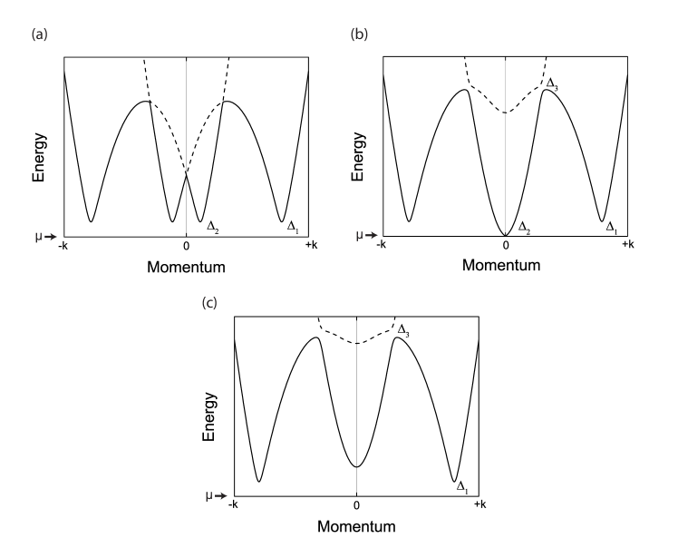
Figure 1: (a) Energy dispersion relation for a nanowire with $M\ll\sqrt{\Delta^{2}+\mu^{2}}$. The solid line corresponds to the relation $\sqrt{E_{t}-2\sqrt{E_{s}}}$ and the dashed line to $\sqrt{E_{t}+2\sqrt{E_{s}}}$. (b) $M=\sqrt{\Delta^{2}+\mu^{2}}$ the gap at $k=0$ is closing. Because of the finite magnetic field there is another gap indicated by $\Delta_{3}$. (c) In the regime $M\gg\sqrt{\Delta^{2}+\mu^{2}}$ a dominant topological non-trivial $p$-wave gap exist at $\Delta_{1}$. The graphs are plotted for $\Delta$ in the order of $\mu$ for clarity.

I.1 Regime $M\ll\sqrt{\Delta^{2}+\mu^{2}}$

In this case we have four superconducting gaps as indicated in Fig. 1(a). $\Delta_{1}$ and $\Delta_{2}$ indicate the position for positive wave vector momentum. At $\Delta_{1}$ (and for the corresponding gap at negative $k$) it follows from the dispersion relation that $\mu=\frac{\hbar^{2}k_{F}^{2}}{2m}-\lambda|k_{F}|$ and for $\Delta_{2}$ $\mu=\frac{\hbar^{2}k_{F}^{2}}{2m}+\lambda|k_{F}|$. Using the relations for the anomolous Green function, Eq. (1), we get for $\Delta_{1}$

$$F_{\upharpoonleft\upharpoonleft}\sim-2\Delta ikk_{f}\lambda^{2}/Z_{nw},$$

$$F_{\upharpoonleft\downharpoonleft}\sim-2\Delta\lambda^{2}k^{2}/Z_{nw},$$

$$F_{\downharpoonleft\upharpoonleft}\sim 2\Delta\lambda^{2}k^{2}/Z_{nw},$$

$$F_{\downharpoonleft\downharpoonleft}\sim 2\Delta ikk_{f}\lambda^{2}/Z_{nw}.$$

Expressions such as $\frac{\hbar^{2}k^{2}}{2m}-\frac{\hbar^{2}k_{F}^{2}}{2m}$ are set to zero in the above equations as we consider low energy excitations. For $\Delta_{2}$ we obtain

$$F_{\upharpoonleft\upharpoonleft}\sim 2\Delta ikk_{f}\lambda^{2}/Z_{nw},$$

$$F_{\upharpoonleft\downharpoonleft}\sim-2\Delta\lambda^{2}k^{2}/Z_{nw},$$

$$F_{\downharpoonleft\upharpoonleft}\sim 2\Delta\lambda^{2}k^{2}/Z_{nw},$$

$$F_{\downharpoonleft\downharpoonleft}\sim-2\Delta ikk_{f}\lambda^{2}/Z_{nw}.$$

We see also here that in the case of time-reversal symmetry there is an equal admixture of $s$ and $p$-wave correlations.

I.2 Regime $M=\sqrt{\Delta^{2}+\mu^{2}}$

This case is shown in Fig. 1(b), where the superconducting gap at $k=0$ is closed. At $\Delta_{2}$ the anomolous Green function parts are zero because $k=0$. Because we have turned on a magnetic field, the bands corresponding to different helicity are not orthogonal anymore. Therefore, there exist an interaction between the two in this regime and another superconducting gap is opening above $\mu$ ($\Delta_{3}$ in the Fig. 1(b)).SanJose2013 For $\Delta_{3}$ the relation $\mu=\frac{\hbar^{2}k^{2}}{2m}$ holds so that

$$F_{\upharpoonleft\upharpoonleft}\sim-2\Delta ik\lambda\mu/Z_{nw},$$

$$F_{\upharpoonleft\downharpoonleft}\sim-\Delta\left(k^{2}\lambda^{2}-\mu^{2}\right)/Z_{nw},$$

$$F_{\downharpoonleft\upharpoonleft}\sim\Delta\left(k^{2}\lambda^{2}-\mu^{2}\right)/Z_{nw},$$

$$F_{\downharpoonleft\downharpoonleft}\sim 2\Delta ik\lambda\mu/Z_{nw}.$$

For a typical Mourik2012 spin orbit strength of $\lambda=0.2$ eV$\cdot$Å and $m=0.015m_{e}$ where $m_{e}$ is the free electron mass, it follows that the magnitude of the spin-singlet order parameters in this regime are larger than the $p$-wave components. However, since the energy level of $\Delta_{3}$ increases with $M$, i.e. $E_{\Delta_{3}}\approx\sqrt{\lambda^{2}k^{2}+M^{2}}$, for low energy excitations this superconducting contribution can be neglected.

At $\Delta_{1}$, $\frac{\hbar^{2}k_{F}^{2}}{2m}-\mu-\sqrt{\lambda^{2}k_{F}^{2}+\mu^{2}}=0$ so that we get the following relations for the anamolous Green function part:

$$F_{\upharpoonleft\upharpoonleft}\sim-2\Delta ik\lambda\left(\mu+\sqrt{\lambda^{2}k_{f}^{2}+\mu^{2}}\right)/Z_{nw},$$

$$F_{\upharpoonleft\downharpoonleft}\sim-2\Delta\lambda^{2}k^{2}/Z_{nw},$$

$$F_{\downharpoonleft\upharpoonleft}\sim 2\Delta\lambda^{2}k^{2}/Z_{nw},$$

$$F_{\downharpoonleft\downharpoonleft}\sim 2\Delta ik\lambda\left(\mu-\sqrt{\lambda^{2}k_{f}^{2}-\mu^{2}}\right)/Z_{nw}.$$

Here, we see that $F_{\downharpoonleft\downharpoonleft}$ becomes gradually smaller and $F_{\upharpoonleft\upharpoonleft}$ becomes larger than the $s$-wave pairing parts, assuming $M$ to be positive. We obtain a dominant $p$-wave component for the spin triplet component where the spins are parallel to the magnetic field.

I.3 Regime $M\gg\sqrt{\Delta^{2}+\mu^{2}}$, “Majorana” regime

The situation is sketched in Fig. 1(c). The gap at $k=0$ reopens. The pairing wave function at $\Delta_{1}$ satisfies

$$F_{\upharpoonleft\upharpoonleft}\sim-2\Delta ik\lambda\left(M+\sqrt{\lambda^{2}k_{f}^{2}+M^{2}}\right)/Z_{nw},$$

$$F_{\upharpoonleft\downharpoonleft}\sim-2\Delta\lambda^{2}k^{2}/Z_{nw},$$

$$F_{\downharpoonleft\upharpoonleft}\sim 2\Delta\lambda^{2}k^{2}/Z_{nw},$$

$$F_{\downharpoonleft\downharpoonleft}\sim 2\Delta ik\lambda\left(M-\sqrt{\lambda^{2}k_{f}^{2}+M^{2}}\right)/Z_{nw}.$$

We see that for increasing $M$ the $p$-wave part becomes more pronounced and that $F_{\upharpoonleft\upharpoonleft}$ becomes larger than $F_{\downharpoonleft\downharpoonleft}$. $F_{\downharpoonleft\downharpoonleft}$ actually goes to zero for increasing positive field. For negative field $F_{\downharpoonleft\downharpoonleft}$ will be dominant as one would expect for the opposite field direction. Around $k=0$ there is no interaction anymore between the hole and electron branches and, as noted before, the degeneracy in the $p$-wave order parameters disappears in this regime.

At $\Delta_{3}$ we have

$$F_{\upharpoonleft\upharpoonleft}\sim-2\Delta ik\lambda M/Z_{nw},$$

$$F_{\upharpoonleft\downharpoonleft}\sim 2\Delta\left(M^{2}-k^{2}\lambda^{2}\right)/Z_{nw},$$

$$F_{\downharpoonleft\upharpoonleft}\sim-2\Delta\left(M^{2}-k^{2}\lambda^{2}\right)/Z_{nw},$$

$$F_{\downharpoonleft\downharpoonleft}\sim 2\Delta ik\lambda M/Z_{nw}.$$

Hence, the $s$-wave pairing becomes dominant for increasing magnetic field at $\Delta_{3}$, but as discussed before it is safe to ignore it in the low excitation regime.

Since the gap at $k=0$ closed for $M=\sqrt{\Delta^{2}+\mu^{2}}$ and has now reopened again we also have a proper localized single Majorana mode at the ends of the nanowire. Just as the surface states of a topological insulator are localized to a surface, the Majorana mode in a nanowire is localized at the ends of the nanowire due to the vacuum gap at one side and the superconducting gap with a reversed band order on the other side. The reversed band order ensures that the bands are crossing at the ends of the nanowire resulting in a localized end mode similar to the topological surface and edge states in topological insulators.

Note, that all of the expressions in this section can be generalized to two dimensions. This could be relevant for InAs thin films for example. The scalar $k$ has to be replaced by a k-vector with an amplitude $|\textbf{k}|$ and phase $e^{i\theta}$ analogous to the 3D topological insulator discussed below. The $e^{i\theta}$ factor denotes the chirality of one branch and $e^{-i\theta}$ the chirality of the other branch present at the Fermi level. Apart from an additional $e^{i\theta}$ and $e^{-i\theta}$ factor in the expressions of the order parameter, the given conclusions would still be valid.

References

• (1) P. San-Jose, J. Cayao, E. Prada, R. Aguado, New Journal of Physics 15, 075019 (2013).
• (2) V.Mourik, K.Zuo, S.M.Frolov, S.R. Plissard, E.P.A.M.Bakkers, L.P.Kouwenhoven, Science 12, 1222360 (2012).