Dynamics of two-cluster systems in phase space

Abstract

We present a phase-space representation of quantum state vectors for two-cluster systems. Density distributions in the Fock–Bargmann space are constructed for bound and resonance states of ^6,7Li and ^7,8Be, provided that all these nuclei are treated within a microscopic two-cluster model. The density distribution in the phase space is compared with those in the coordinate and momentum representations. Bound states realize themselves in a compact area of the phase space, as also do narrow resonance states. We establish the quantitative boundaries of this region in the phase space for the nuclei under consideration. Quantum trajectories are demonstrated to approach their classical limit with increasing energy.

1 Introduction

The idea of formulation of quantum mechanics in a phase space is discussed in numerous theoretical papers [1, 2, 3, 4, 5, 6]. The majority of such investigations are concentrated on establishing the link between quantum and classical mechanics. Due to the uncertainty principle there is no unique definition of the phase space. By this reason, different quantum phase space distribution have been proposed. In particular, in the phase-space representation of Wigner and Husimi a quantum state is represented by a distribution function (see the definitions, for instance, in [1, 2]), and the equations of motion are of the Liouville type.

A state-vector representation is another possibility to describe the dynamics of a quantum system in phase space. In this case a quantum state is represented by a wave function, and the equations of motion are of the Schrödinger type. The definition of the phase-space representation is related to the choice of an operator which should be diagonal in this representation. In the coordinate representation the coordinate operator is diagonal, while the momentum operator is non-local. At the same time, the momentum representation diagonalizes the momentum operator, and the coordinate operator is non-local. Obviously, the coordinate operator and the momentum operator can not be diagonal simultaneously due to the uncertainty principle. Hence, one should seek for another operator.

In Ref. [3], mention was made that representation of a quantum state as a probability amplitude depending on two real variables related to the coordinate and momentum dates back to the papers of Fock [7] and Bargmann [8]. In the Fock-Bargmann space, a quantum state is represented as an entire function of a complex variable, with real and imaginary part of this variable being proportional to the coordinate and momentum, correspondingly. The Fock-Bargmann representation diagonalizes the creation operator, while the annihilation operator is non-local.

A quantum problem can be resolved in any one of the above-mentioned representations. The Fock-Bargmann image of a wave function can be obtained from the wave function in the coordinate representation by a linear mapping, while the Husimi and the Wigner distribution functions are bilinear with respect to the wave function in the coordinate representation. However, the Fock-Bargmann representation is closely related to the Husimi distribution. The latter distribution is equal to the square of the Fock-Bargmann image of the corresponding wave function multiplied by the Bargmann measure.

In Refs. [4, 5], Torres-Vega and Frederic suggested a quantum-state vector phase-space representation. The authors postulated the existence of a complete basis of states $|q,p\rangle$ such that in the phase space a quantum state $|\psi\rangle$ is represented by an $\mathcal{L}^{2}(2)$ wave function $\psi(p,q)=\langle q,p|\psi\rangle.$ Here $q,p$ are real values and the operators of coordinate and momentum in this basis take the form:

$$\widehat{Q}={\frac{q}{2}}+\imath\hbar{\frac{\partial}{\partial p}},~{}~{}~{}\widehat{P}={\frac{p}{2}}-\imath\hbar{\frac{\partial}{\partial q}}.$$ (1)

Thus Torres-Vega and Frederic developed a wave-function formulation of quantum mechanics in a phase space. Wave functions are governed by the Schrödinger equation in the phase space, while square of absolute value of the wave function plays the role of the probability density in the phase space obeying the Liouville equation. However, the quantum-state vector phase-space representation is not uniquely defined, because there exists an infinite number of bases depending on two real variables $p,q$ which result in the foregoing expression of the coordinate and momentum operators $\widehat{Q}$ and $\widehat{P}$.

In Ref. [5], the authors used coherent states as basis vectors and demonstrated that any coherent state representation leads to expression (1) for the coordinate and momentum operators $\widehat{Q}$ and $\widehat{P}$. Moreover, they concluded that only the coherent state representation makes it possible to define the operators of coordinate and momentum in such a manner.

Following Klauder and Perelomov, in [5] a set of coherent states is defined as a result of action of the Weyl operator $\widehat{D}(q,p)$ (a translation operator in the phase space)

$$\widehat{D}(q,p)=\exp\left\{{\frac{i}{\hbar}}\left(p\,\widehat{Q}-q\widehat{P}\right)\right\}$$

to any normalized vector $|\chi\rangle:$

$$|q,p;\chi\rangle\equiv\widehat{D}(q,p)|\chi\rangle.$$

For any fixed vector $|\chi\rangle$ the set of coherent states $|q,p;\chi\rangle$ ensures a continuous representation of quantum states where the expansion coefficients can be interpreted as the wave function in the phase space.

Then $|\psi_{\chi}(q,p)|^{2}$ is a ”dilute” probability density in the phase space that equals the probability for a system to be localized in some ”dilute” neighborhood of the center of the displaced state $\chi$. The degree of ”diffusiveness” depends on the choice of vector $\chi$. If we choose the ground state of a harmonic oscillator as the vector $\chi$ then $|\psi_{\chi}(q,p)|^{2}$ is probability to find a system in the elementary phase volume $\Delta q\Delta p=h$ near the point $(q,p)$.

The Schrödinger equation in the phase space does not depend explicitly on the vector $\chi.$ However, in calculating mean values of operators the wave functions used for averaging should belong to the same coherent state representation, i.e., to the same vector $\chi$. This could be ensured by the requirement for the vector $\chi$ to be an eigenvector of a certain operator. Hence, to formulate quantum mechanics unambiguously, one should solve two equations in the phase space.

It is possible to formulate quantum mechanics in a phase space so that one equation could be sufficient both for the solution of a quantum problem and for specification of the representation. As concluded in [5], the Fock-Bargmann representation suggests the best answer to this question. The Fock-Bargmann representation is a state-vector representation in the complex plane which is based on the mapping of the pair of bosonic creation and annihilation operators $(\widehat{a},\widehat{a}^{{\dagger}}):$

$$\widehat{a}\rightarrow{\frac{\partial}{\partial R}},\,\,\,{\widehat{a}}^{{\dagger}}\rightarrow R.$$ (2)

In this representation quantum mechanics can be uniquely determined due to the fact that the creation operator $\widehat{a}^{{\dagger}}$ is diagonal in this representation. The relation $[\widehat{a},\widehat{a}^{{\dagger}}]=1$ is followed by the relationships between the bosonic operators and the coordinate and momentum operators $\widehat{Q}$ and $\widehat{P}$:

$$\widehat{a}={\frac{1}{\sqrt{2}}}\left({\frac{1}{b}}\widehat{Q}-i{\frac{b}{\hbar}}\widehat{P}\right),\,\,\widehat{a}^{{\dagger}}={\frac{1}{\sqrt{2}}}\left({\frac{1}{b}}\widehat{Q}+i{\frac{b}{\hbar}}\widehat{P}\right),$$

where $b$ is the oscillator length.

For a specific hamiltonian $\widehat{H}(\widehat{Q},\widehat{P})$ one can fix the relationship between the operators $\widehat{Q}$, $\widehat{P}$ and bosonic operators $(\widehat{a},\widehat{a}^{{\dagger}})$ by choosing the value of the oscillator length $b$. Then the Hamiltonian can be expressed in terms of the bosonic operators $\widehat{H}(\widehat{Q},\widehat{P})\rightarrow\mathcal{H}(\widehat{a},\widehat{a}^{{\dagger}})$. Hence, the vector $\chi$ is completely determined by the value of $b$. In this case the vector $\chi$ is the vacuum vector $|0\rangle$.

The Fock-Bargmann representation can be associated with any Glauber coherent state representation based on the eigenvector $\chi$ of the annihilation operator $a.$ According to Perelomov [9], a coherent state describes a non-spreadable wave packet for an oscillator. Besides, coherent states minimize the Heisenberg uncertainty relation $\Delta q\Delta p\geq h.$ Hence the coherent states are quantum states which resemble classic states the most. The Schrödinger equation in the Fock-Bargmann representation has the form:

$$i\hbar{\frac{\partial}{\partial t}}|\psi\rangle=\mathcal{H}(\widehat{a},\widehat{a}^{{\dagger}})|\psi\rangle\rightarrow i\hbar{\frac{\partial}{\partial t}}\psi_{FB}(R)=\mathcal{H}\left({\frac{\partial}{\partial R}},R\right)\psi_{FB}(R),$$ (3)

where

$$R={\frac{1}{\sqrt{2}}}\left({\frac{q}{b}}+i{\frac{b}{\hbar}}p\right).$$

Hence, a complete basis of the wave functions belonging to the class of coherent states which minimize the uncertainty relation can be unambiguously determined as a result of solution of the Schrödinger equation in the Fock-Bargmann representation (2).

We follow precisely this strategy and present the wave functions and the probability distributions in the Fock-Bargmann representation. However, we don’t solve an equation of the type (3), we use other way for obtaining an exact wave function of a quantum system. We concentrate our attention on the analysis of nuclear systems with a pronounced two-cluster structure, whereas authors of Refs. [3, 5] have studied one-dimensional systems wherein the solutions could be found analytically. Much prominence is given to the determination of those regions of phase space, which are the most important for the dynamics of two-cluster systems. We also suggested the way of investigation of the density distributions in the phase space in a three-dimensional case, when the probability density distribution depends on six variables: absolute values of coordinate and momentum and four angles.

There are some similarities between our approach and the Antisymmetrized Molecular Dynamics (AMD) [10, 11] and the Fermionic Molecular Dynamics (FMD) [12, 13]. The AMD and FMD have been intensively employed to study a cluster structure of atomic nuclei and both of them appeal to a phase space. All three methods make use the same single particle orbitals to construct a many-particle wave function in the form of the Slater determinant. It means that all methods involve the same part of the total Hilbert space, provided that all of them take into account the same partition (or clusterization) of $A$ nucleon system. However, there are more differences between our approach and AMD and FMD. First, we use the Slater determinants as the generation functions for a complete basis of many-particle oscillator functions, describing the most important, from physical point of view, types of motion of many-particle system. In our approach cluster parameters are the generator coordinates that allow us to select necessary basis functions from the infinite set of oscillator functions. Meanwhile, in the AMD and FMD they are independent variables in the phase space. By using a set of many-particle oscillator functions, we reduce the Schrödinger equation to the matrix form. The AMD and FMD make use of the time-dependent equations derived from the time-dependent variational principle. Having obtained the wave function in a discrete, oscillator representation, we then transform it to the Fock-Bargmann or phase space, where we analyze phase trajectories of a quantum many-particle system.

It should be emphasized that all the results presented in this paper are obtained within the phase-space formulation of quantum mechanics which is valid both for finite $\hbar$ and when $\hbar$ goes to zero. We consider some simple model cases as well as two-cluster systems. The model cases, such as a three-dimensional harmonic oscillator and a plane wave, help us to reveal peculiarities of phase space portraits. However, our main aim is to study phase portraits of real physical systems, namely, light atomic nuclei. All calculations are performed within a microscopic two-cluster model based on the resonating-group method (RGM) [14]. Our analysis started from assumptions of the following cluster structure of the nuclei under consideration: ${}^{6}Li=\alpha+d$, ${}^{7}Li=\alpha+t$, ${}^{7}Be=\alpha+^{3}He$, ${}^{8}Be=\alpha+\alpha$. Instead of solving an integro-differential equation in a phase space as the authors of Ref. [4] do, we deal with the RGM Hamiltonian in the representation of the Pauli-allowed harmonic-oscillator states defined in the Fock–Bargmann space. Doing so, we reduce the integro-differential equation to a set of linear equations for coefficients of the expansion of the wave function in the harmonic-oscillator basis.

Our paper is organized as follows. In Section 2 we introduce all necessary definitions and formulate an approach for constructing density distributions in the Fock-Bargmann space. In Section  3, the effectiveness of the suggested approach is demonstrated for two simple model problems: a harmonic oscillator and a free motion in 3D space. In Section 4 we give a brief review of the employed two-cluster model. Details of the calculations are shown in Section 5. Phase portraits for bound and resonance states in the light atomic nuclei are presented in Section 6. Finally, in Section 7 we conclude the main results obtained.

2 The Fock-Bargmann representation

In this section and Section 3 we shall use dimensionless units for energy and length. The energy $E$ is measured in units of $\frac{\hbar^{2}}{mb^{2}}$ and the length is measured in terms of oscillator length $b.$ The value of the oscillator length will be determined in what follows.

The transition from the wave function in the coordinate or momentum representation to the wave function in the Fock–Bargmann representation is performed using the Bargmann-Segal integral transformation

$$\Psi_{E}(\mathbf{R})=\int K(\mathbf{R},\mathbf{r})\Psi_{E}(\mathbf{r})d\mathbf{r},~{}~{}\mathbf{R}={\frac{\vec{\xi}+i\vec{\eta}}{\sqrt{2}}},$$ (4)

the kernel of which is the modified Bloch-Brink orbitals [15]:

$$K(\mathbf{R},\mathbf{r})={\frac{1}{{\pi^{3/4}}}}\exp\left(-{\frac{r^{2}}{2}}+\sqrt{2}\,(\mathbf{rR})-{\frac{R^{2}}{2}}\right).$$ (5)

In the Fock-Bargmann space, wave functions are entire analytical functions of complex variable $\mathbf{R}$, while $\vec{\xi}$ and $\vec{\eta}$ are coordinate and momentum vectors, respectively.

The modified Bloch—Brink orbital is an eigenfunction of the coordinate operator in the Fock-Bargmann space:

$$\widehat{\mathbf{r}}K(\mathbf{R},\mathbf{r})=\mathbf{r}K(\mathbf{R},\mathbf{r}),~{}~{}~{}~{}\widehat{\mathbf{r}}={\frac{1}{\sqrt{2}}}\left(\mathbf{R}+\nabla_{\mathbf{R}}\right).$$

On the other hand, the modified Bloch-Brink orbital is a coherent state and generates a complete basis of functions of a 3D-harmonic oscillator.

Having calculated the wave function in the Fock-Bargmann space, we can find the density distribution, which depends on six variables: absolute values of the coordinate and momentum $\xi$, $\eta$ and four angles $\Omega_{\vec{\xi}}$, $\Omega_{\vec{\eta}}$:

$$dD_{E}(\vec{\xi},\vec{\eta})=|\Psi_{E}(R)|^{2}d\mu_{B}=|\Psi_{E}(\mathbf{R})|^{2}\exp\left({-\frac{\eta^{2}+\xi^{2}}{2}}\right){\frac{d\vec{\xi}d\vec{\eta}}{(2\pi)^{3}}}.$$ (6)

Here

$$d\mu_{B}=\exp\{-(\mathbf{R}\cdot\mathbf{S})\}{\frac{d\vec{{\xi}}d\vec{{\eta}}}{(2\pi)^{3}}},~{}~{}\mathbf{S}=\mathbf{R}^{\ast}$$

is the Bargmann measure.

In essence, $dD_{E}(\vec{\xi},\vec{\eta})$ is a density matrix in the Fock-Bargmann space. It is positively defined for all values of $\vec{\xi}$ and $\vec{\eta}$ as opposed to the Wigner function, which is often used to construct a density distribution in a phase space. In fact, $D_{E}(\vec{\xi},\vec{\eta})$ coincides with the Husimi distribution within definition of variables $\vec{\xi}$ and $\vec{\eta}$.

It is rather difficult to investigate the density distribution $D_{E}(\vec{\xi},\vec{\eta}),$ because it depends on six variables. To solve this problem and extract as much as possible physical information, we propose to integrate $D_{E}(\vec{\xi},\vec{\eta})$ over the solid angles $\Omega_{\vec{\xi}}$ and $\Omega_{\vec{\eta}}$. Then we come out with the density distribution $D_{E}(\xi,\eta)$ which depends only on the absolute values of the coordinate and momentum.

$$D_{E}(\xi,\eta)\equiv{\frac{\int d\Omega_{\vec{\xi}}\int d\Omega_{\vec{\eta}}\,dD_{E}(\vec{\xi},\vec{\eta})}{d\xi d\eta}}.$$

It is important to recall, that the variable $\xi$ is analogue of the distance between interacting particles (clusters) and the variable $\eta$ represents a momentum of relative motion of particles (clusters).

Given the energy $E$ and other integrals of motion, like the orbital momentum and parity, the density distribution $D_{E}(\xi,\eta)$ is comprised of the infinite number of phase trajectories. The phase trajectories are determined as a continuous set of points in the $(\xi,\eta)$ plane for the fixed values of the density distribution $D_{E}(\xi,\eta)=const$, while the probability of realization of the phase trajectory is proportional to the values of $D_{E}(\xi,\eta)$. Hereinafter we shall call an infinite set of phase trajectories characterizing a particular quantum state of the system under study the phase portrait.

With increase in energy $E$, all the quantum phase trajectories gradually approach their classical limit. Therefore, analyzing phase portraits of quantum systems we can make a quantitative estimate of the energy such that the maximum of the density distribution $D_{E}(\xi,\eta)$ falls on the classical trajectory.

In [16], we have constructed and analyzed the phase portraits for the free motion of a 1D quantum particle and for the motion in the field of Gaussian potential. In the present paper we concentrate on the three-dimensional case. Before proceeding to the analysis of phase portraits of two-cluster systems, let us discuss the density distribution for the states of a three-dimensional oscillator with the number of quanta $N$ and for a free motion of a 3D-particle in the states with the orbital momentum $l.$

3 Model problems

3.1 Harmonic oscillator

The overlap integral of the modified Bloch-Brink orbitals

$$\langle\mathbf{S}|\mathbf{R}\rangle\equiv\int K(\mathbf{S},\mathbf{r})K(\mathbf{R},\mathbf{r})d\mathbf{r}=\exp(\mathbf{R}\mathbf{S})$$

generates a complete basis for the harmonic-oscillator functions in the Fock-Bargmann representation:

$$\exp(\mathbf{R}\mathbf{S})=\sum_{n=0}^{\infty}\sum_{l}N_{nl}^{2}R^{2n+l}S^{2n+l}\sum_{m}Y_{lm}(\Omega_{R})Y_{lm}^{\ast}(\Omega_{S})$$ (7)

Here both the absolute value and the solid angle of the complex vector $\mathbf{R}$ take complex values:

$$R=\sqrt{\mathbf{R}^{2}}=\sqrt{\frac{1}{2}}\sqrt{\left({\xi^{2}-\eta^{2}}\right){+2i(\vec{\xi}\vec{\eta})}},\,\,\,\,\Omega_{R}={\frac{\mathbf{R}}{R}}={\frac{\vec{\xi}+i\vec{\eta}}{\sqrt{\left(\xi^{2}-\eta^{2}\right)+2i(\vec{\xi}\vec{\eta})}}}$$

Each basis function corresponds to the total number of quanta $N=2n+l,$ where $l$ is the orbital momentum and $n$ is the number of radial quanta:

$$|n,l,m;\mathbf{R}\rangle=N_{nl}R^{2n+l}Y_{lm}(\Omega_{R}),\,\,\,N_{nl}=\sqrt{{\frac{4\pi}{(2n)!!(2n+2l+1)!!}}}.$$ (8)

Hence, according to the definition (6), a density distribution for the $|n,l;\mathbf{R}\rangle$ state of harmonic oscillator should be written as

$$dD_{n,l}(\vec{\xi},\vec{\eta})={\frac{1}{2l+1}}\sum_{m}|n,l,m;\mathbf{S}\rangle\langle n,l,m;\mathbf{R}|\,d\mu_{B}.$$

Here averaging over projection $m$ of the orbital momentum is performed.

Integrating over the solid angles related to the coordinate $\vec{\xi}$ and momentum $\vec{\eta}$, we come to the expression

$$D_{n,l}(\xi,\eta) = {\frac{\xi^{2}\eta^{2}}{(2\pi)^{3}}}\int d\Omega_{\xi}\int d\Omega_{\eta}dD_{n,l}(\vec{\xi},\vec{\eta})={\frac{\xi^{2}\eta^{2}}{2\pi^{2}}}\,{\frac{N_{nl}^{2}}{2^{2n+l}}}\,e^{-{(\xi^{2}+\eta^{2})/2}}\times$$

$$\times \sum_{\nu=0}^{\left[{\frac{l}{2}}\right]}d_{\nu}^{l}(\xi^{2}-\eta^{2})^{2n+2\nu}(\xi^{2}+\eta^{2})^{l-2\nu}$$

$$\times \,{}_{2}F_{1}\left(-n-\nu,{\frac{1}{2}},{\frac{3}{2}};-{\frac{4(\xi\eta)^{2}}{(\xi^{2}-\eta^{2})^{2}}}\right),$$

where

$$d_{\nu}^{l}={\frac{(-1)^{\nu}(2l-2\nu)!}{2^{l}\nu!(l-\nu)!(l-2\nu)!}}.$$

As observed in the right panel of Fig. 1, with increase in the orbital momentum $l$ the density distribution $D_{n,l}(\xi,\eta)$ is slightly forced out from the region of small $\xi$ and $\eta$ and narrows.

The left panel of Fig. 1 demonstrates that the density distributions $D_{n,l}(\xi,\eta)$ corresponding to the same total number of quanta $N$, but different orbital momenta $l,$ peak on the same circle:

$${\frac{\xi^{2}+\eta^{2}}{2}}=2n+l+2.$$ (9)

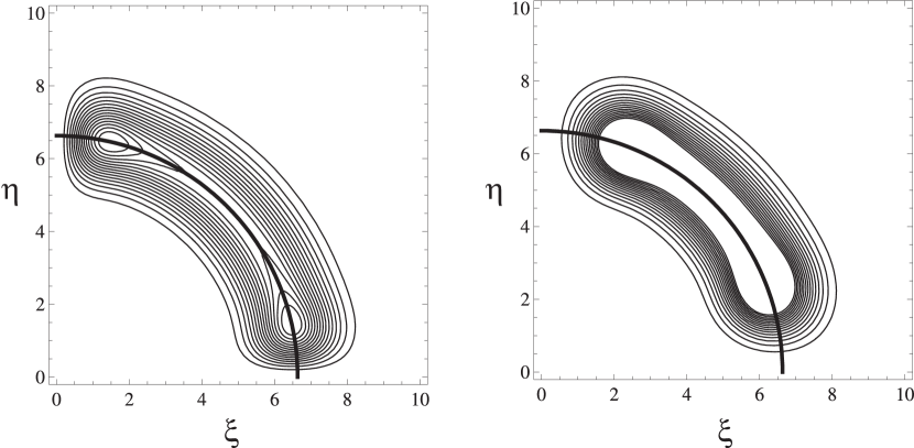
Figure 1: Phase portraits of a 3D oscillator $D_{n,l}(\xi,\eta)=const$ with the total number of quanta $2n+l=20$ as a function of dimensionless coordinate $\xi$ and momentum $\eta$. The left panel corresponds to $D_{n=10,l=0}(\xi,\eta)=const,$ the right panel demonstrates $D_{n=5,l=10}(\xi,\eta)=const$. The heavy line on both panels denotes the classical trajectory defined by Eq. (9).

Eq. (9) describes a classical trajectory of the particle with the energy $E_{cl}=2n+l+2.$ Hence, the most probable locus of points in the phase space for the eigenstate of a 3D harmonic oscillator with the number of quanta $N=2n+l$ corresponds to the classical energy $E_{cl}=N+2$ rather than to $E_{cl}=N+3/2.$ The maximum of density distribution for the $N$th state of a 1D harmonic oscillator was matched by the classical energy $E_{cl}=N$ instead of $E_{cl}=N+1/2$ (see [4, 16]).

3.2 Plane wave

In the Fock-Bargmann representation, a plane wave corresponding to the momentum $\mathbf{k}$ becomes:

$$\phi_{\mathbf{k}}(\mathbf{R})=\pi^{-3/4}\exp\left\{-{\frac{k^{2}}{2}}-i\sqrt{2}(\mathbf{kR})+{\frac{R^{2}}{2}}\right\}.$$ (10)

It is an eigenfunction of the momentum operator $\widehat{\mathbf{k}}$:

$$\widehat{\mathbf{k}}\phi_{\mathbf{k}}(\mathbf{R})=\mathbf{k}\phi_{\mathbf{k}}(\mathbf{R}),~{}~{}~{}~{}\widehat{\mathbf{k}}=-{\frac{i}{\sqrt{2}}}\left(\mathbf{R}-\nabla_{\mathbf{R}}\right).$$

The density distribution for the plane wave (10) has the Gaussian dependence on the momentum $\eta$ and is unaffected by the coordinate $\xi:$

$$dD_{\mathbf{k}}(\vec{\xi},\vec{\eta})=|\phi_{\mathbf{k}}(\mathbf{R})|^{2}d\mu_{B}=\pi^{-3/2}\exp\left(-(\mathbf{k}-{\vec{\eta}})^{2}\right){\frac{d\vec{\xi}d\vec{\eta}}{(2\pi)^{3}}}.$$ (11)

Obviously, the density distribution (11) peaks on the line ${\vec{\eta}}=\mathbf{k}$. This line coincides with the classical phase trajectory of a free particle with momentum $\mathbf{k}.$

The problem becomes more intricate if we consider free motion of a particle in the states with given value of the orbital momentum $l$. We can expand the eigenfunction (10) of the momentum operator $\widehat{k}$ in the basis of the harmonic oscillator functions (8) in the Fock-Bargmann space:

$$\phi_{\mathbf{k}}(\mathbf{R})=\sum_{n=0}^{\infty}\sum_{l}\sum_{m}|n,l,m;\mathbf{R}\rangle C_{nl}(k)Y_{lm}(\Omega_{k}).$$ (12)

Expansion (12) in the Fock-Bargmann representation is much the same as the multipole expansion of the plane wave in the coordinate representation.

The expansion coefficients $C_{nl}(k)$ coincide with the basis functions of harmonic oscillator in the momentum representation. In particular, for zero orbital momentum the expansion coefficients $C_{nl}(k)$ are defined as

$$C_{n,l=0}(k)=\sqrt{{\frac{2\Gamma(n+1)}{\Gamma(n+3/2)}}}L_{n}^{1/2}(k^{2})\exp\left(-{\frac{k^{2}}{2}}\right).$$ (13)

Generally in the Fock-Bargmann space any wave function $\Psi_{lm}^{E}(\mathbf{R})$ of a quantum state characterized by the orbital momentum $l,$ its projection $m$ and energy $E$ can be represented as the expansion into the basis of the harmonic oscillator functions (8):

$$\Psi_{lm}^{E}(\mathbf{R})=\sum_{n=0}^{\infty}\sum_{l}C_{nl}^{E}|n,l,m;\mathbf{R}\rangle,$$ (14)

where the expansion coefficients $C_{nl}^{E}$ are the solutions of a set of linear algebraic equations to which the Schrödinger equation is reduced. The expansion (14) is written in the Fock-Bargmann space; it can be also presented in coordinate and momentum spaces with the same set of the expansion coefficients $\left\{C_{nl}^{E}\right\}$. Such way of representing and calculating the wave functions is the essence of the method we follow in the present paper.

Hence, the density distribution for the quantum state described by the wave function $\Psi_{lm}^{E}(\mathbf{R})$ takes the form:

$$dD_{E,l}(\vec{\xi},\vec{\eta})={\frac{1}{2l+1}}\sum_{n=0}^{\infty}\sum_{\tilde{n}=0}^{\infty}\sum_{m}C_{nl}^{E}C_{\tilde{n}l}^{E}|k,l,m;\mathbf{S}\rangle\langle k,l,m;\mathbf{R}|\,d\mu_{B}.$$

Upon integrating the foregoing expression over the solid angles $\Omega_{\vec{\xi}}$ and $\Omega_{\vec{\eta}}$ we obtain:

$$D_{E,l}(\xi,\eta) = {\frac{\xi\eta}{2\pi^{2}}}(\xi^{2}-\eta^{2})\,\exp\left(-{\frac{\xi^{2}+\eta^{2}}{2}}\right)\,\sum_{n=0}^{\infty}\sum_{\tilde{n}=0}^{\infty}N_{nl}N_{\tilde{n}l}C_{nl}^{E}C_{\tilde{n}l}^{E}\times$$

$$\times \sum_{\nu=0}^{\left[{\frac{l}{2}}\right]}d_{\nu}^{l}\left({\frac{\xi^{2}+\eta^{2}}{2}}\right)^{l-2\nu}(\xi^{2}-\eta^{2})^{n+\tilde{n}+2\nu}$$

$$\times Im\left[B\left({\frac{1}{2}}+i{\frac{\xi\eta}{\xi^{2}-\eta^{2}}};n+\nu+1,\tilde{n}+\nu+1\right)\right],$$

where $B(z;a,b)$ is the incomplete beta function.

Substituting the coefficients (13) in the formula given above we derive the density distribution for a free motion of the particle with zero orbital momentum. Figure 2 demonstrates the phase portraits for a free particle with $k=1$ and $k=5.$

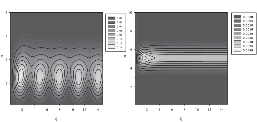
Figure 2: Phase portraits of a free 3D particle with the energy $E=k^{2}/2$ and zero orbital momentum as a function of the dimensionless coordinate $\xi$ and momentum $\eta$. The left panel corresponds to $k=1$, while the right panel corresponds to $k=5.$

As observed in Fig. 2, for $k=1$ the density distribution oscillates in the variable $\xi$. These oscillations, resulting in a number of closed trajectories, are of quantum nature. With increasing the energy the density distribution becomes smoother; all the quantum trajectories become infinite and approach the classical trajectory $\eta\simeq k.$

Figure 3 compares the density distributions in the Fock-Bargmann space, coordinate representation and momentum representation for a free 3D particle with the energy $E=k^{2}/2$, $k=1$ and zero orbital momentum.

In the coordinate representation the wave function of a free particle in the state with $l=0$ is described by the spherical Bessel function $\psi_{k}\left(r\right)=\sqrt{2/\pi}j_{0}(kr),$ while in the momentum representation it is just the Dirac delta-function $\psi_{k}\left(p\right)=\delta(p-k)$. As is clear from Fig. 3, locations of the maxima for the density distributions in the variable $\xi$ in the Fock-Bargmann and coordinate representations almost coincide, while the density distribution in the variable $\eta$ peaks at $\eta\simeq 1.25$ instead of $\eta=1$ as the momentum density distribution does.

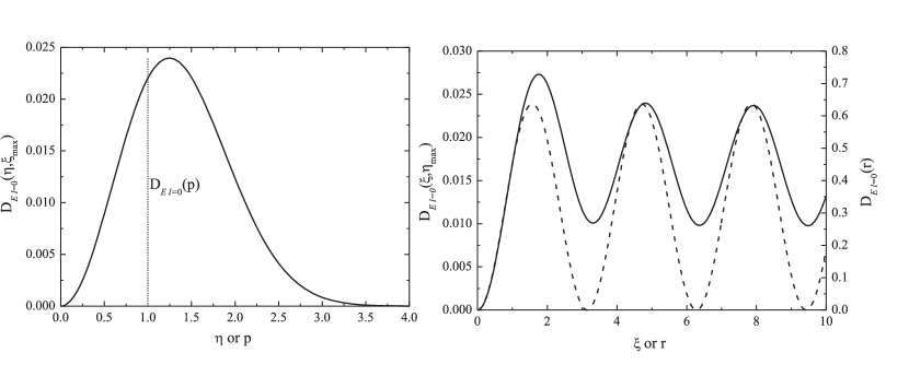
Figure 3: The left panel presents the density distributions $D_{E,l=0}(\xi_{max},\eta)$ in the phase space (a solid line) and $D_{E,l=0}(p)$ in the momentum space (a dashed line) for a free 3D particle with the energy $E=k^{2}/2,$ $k=1$ and zero orbital momentum. The right panel shows the density distributions $D_{E,l=0}(\xi,\eta_{max})$ in the phase space (a solid line) and $D_{E,l=0}(p)$ in the coordinate space (a dashed line).

4 Two-cluster model of light nuclei

We present shortly main ideas of the two-cluster model that we are going to use to study the dynamics of two-cluster systems. First of all, we restrict ourselves with the lightest nuclei of $p$-shell.

A wave function for the two-cluster partition $A=A_{1}+A_{2}$ is represented as

$$\Psi_{J}=\widehat{\mathcal{A}}\left\{\left[\Phi_{1}\left(A_{1}\right)\Phi_{2}\left(A_{2}\right)\right]_{S}\psi_{LS}^{J}\left(q\right)Y_{L}\left(\widehat{\mathbf{q}}\right)\right\}_{J},$$ (15)

where $\widehat{\mathcal{A}}$ is the antisymmetrization operator, $\mathbf{q}$ is the Jacobi vector which is proportional to the vector $\mathbf{r}$ connecting the centers of mass of the interacting clusters

$$\mathbf{q}=\mathbf{r}\sqrt{\frac{A_{1}A_{2}}{A_{1}+A_{2}}}=\sqrt{\frac{A_{1}A_{2}}{A_{1}+A_{2}}}\left[\frac{1}{A_{1}}\sum_{i\in A_{1}}\mathbf{r}_{i}-\frac{1}{A_{2}}\sum_{j\in A_{2}}\mathbf{r}_{j}\right].$$ (16)

It is assumed that the number of nucleons in each cluster $A_{i}$ does not exceed 4: 1$\leq A_{i}\leq$4 . As one sees, we use the $LS$ scheme of coupling, when the total spin $S$ is coupled with the total orbital momentum $L$ and generates the total angular momentum $J$. For two interacting $s$-clusters, the total orbital momentum $L$ coincides with the angular momentum of the relative motion of clusters.

To find the wave function $\psi_{LS}^{J}\left(q\right)$ of relative motion of the clusters one has to solve a set of integro-differential equations (see the details in Ref. [17]). The set of equations and the form of the wave function (15) are the key elements of the well known Resonating Group Method.

An integral part of the integro-differential equations for the functions $\psi_{LS}^{J}\left(q\right)$ is due the to the antisymmetrization operator $\widehat{\mathcal{A}}$ and originates from the potential, and kinetic energy operators, and the norm kernel. The latter means that interaction between clusters is energy dependent. By neglecting the operator $\widehat{\mathcal{A}}$, we obtain differential equations with a local potential. This approximation is called the folding approximation or the folding model.

The Form and procedure of solving the equations for the functions $\psi_{LS}^{J}\left(q\right)$ can be simplified, if we use a set of square-integrable functions. Such way of solving the equations of the Resonating Group Method with oscillator functions is called an Algebraic Version of the Resonating Group Method [18, 19]. To realize the algebraic version, we introduce a set of cluster oscillator functions

$$\left|n,L,S,J\right\rangle=\widehat{\mathcal{A}}\left\{\left[\Phi_{1}\left(A_{1}\right)\Phi_{2}\left(A_{2}\right)\right]_{S}\Phi_{nL}\left(q\right)Y_{L}\left(\widehat{\mathbf{q}}\right)\right\}_{J},$$ (17)

where

$$\Phi_{nL}\left(r,b\right) = \left(-1\right)^{n}\mathcal{N}_{nL}~{}b^{-3/2}\rho^{L}e^{-\frac{1}{2}\rho^{2}}L_{n}^{L+1/2}\left(\rho^{2}\right),\quad$$ (18)

$$\rho = \frac{r}{b},\quad\mathcal{N}_{nL}=\sqrt{\frac{2\Gamma\left(n+1\right)}{\Gamma\left(n+L+3/2\right)}}$$

is an oscillator function in the coordinate space ($b$ is the oscillator length). We are interested in wave functions and density distributions both in the coordinate and in momentum space. They will be constructed with the help of the oscillator functions in the momentum space

$$\Phi_{nL}\left(p,b\right) = \mathcal{N}_{nL}~{}b^{3/2}\rho^{L}e^{-\frac{1}{2}\rho^{2}}L_{n}^{L+1/2}\left(\rho^{2}\right),$$ (19)

$$\quad\rho = p\cdot b,$$

The cluster oscillator functions $\left|n,L,S,J\right\rangle$ are totally antisymmetric and compose a complete set of basis functions with specific physical properties. Namely, they are a part of the total Hilbert space describing the $A_{1}+A_{2}$ clusterization of the system of $A$ nucleons with fixed internal clusters functions $\Phi_{1}\left(A_{1}\right)$ and $\Phi_{2}\left(A_{2}\right)$. The cluster oscillator functions can be used to expand any wave function of the type (15):

$$\Psi_{J}=\sum_{LS}\sum_{n=0}^{\infty}C_{nL}\left|n,L,S,J\right\rangle.$$ (20)

The expansion coefficients $\left\{C_{nL}\right\}$ represent a two-cluster wave function in a discrete, oscillator representation and obey the system of linear equations

$$\sum_{LS}\sum_{m=0}^{\infty}\left[\left\langle n,L,S,J\left|\widehat{H}\right|m,L,S,J\right\rangle-E\cdot\left\langle n,L,S,J|m,L,S,J\right\rangle\right]C_{mL}=0,$$ (21)

where $\left\langle n,L,S,J\left|\widehat{H}\right|m,L,S,J\right\rangle$ is a matrix element of the hamiltonian between the cluster oscillator functions and $\left\langle n,L,S,J|m,L,S,J\right\rangle$ is an overlap of these functions or the norm kernel. For two $s$-clusters, the norm kernel has a very simple form

$$\left\langle n,L,S,J|m,L,S,J\right\rangle=\delta_{n,m}\lambda_{n}.$$ (22)

The constants $\lambda_{n}$ are the eigenvalues of the antisymmetrization operator. The states $\left|n,L,S,J\right\rangle$ with $\lambda_{n}=0$ are called the Pauli-forbidden states. The antisymmetric basis functions with the quantum numbers $n,L,S,J$ do not participate in constructing the wave function (15). Only the Pauli-allowed states (i.e., the states with $\lambda_{n}>0$) take part in describing the dynamics of the two-cluster system.

Equation (22) indicates that the cluster oscillator functions (17) are not normalized to unity despite the fact that the functions $\Phi_{1}\left(A_{1}\right)$, $\Phi_{2}\left(A_{2}\right)$, $\Phi_{nL}\left(q\right)$ and $Y_{LM}\left(\widehat{\mathbf{q}}\right)$ are properly normalized. The antisymmetrization operator $\widehat{\mathcal{A}}$ is responsible for that. By renormalizing the basis functions

$$\left|\overline{n,L,S,J}\right\rangle=\left|n,L,S,J\right\rangle/\sqrt{\lambda_{n}}$$

and the expansion coefficients $\overline{C}_{nL}=C_{nL}\sqrt{\lambda_{n}}$, we arrive at the standard matrix form of the Schrödinger equation with the orthonormal basis

$$\sum_{LS}\sum_{m}\left[\left\langle\overline{n,L,S,J}\left|\widehat{H}\right|\overline{m,L,S,J}\right\rangle-E\cdot\delta_{n,m}\right]\overline{C}_{mL}=0,$$ (23)

where $n$ and $m$ numerates only the Pauli-allowed states.

Formally, the expansion (20) of the wave function contains an infinite set of basis functions; however, actually we need a large but restricted set of functions. In an oscillator representation, situation is similar to the coordinate form of the Schrödinger equation where one needs to find a wave function up to a finite distance $R_{a}.$ Beyond this point the well-known asymptotic form of the wave function is valid. $R_{a}$ determine a distance where a short-range interaction is negligibly small and an asymptotic part of the hamiltonian is dominant. The same is true for the discrete representation. We need to calculate the wave function up to the finite value of $n=N_{a}$; starting from this number of quanta an asymptotic form for the expansion coefficients of the wave function is valid. Like $R_{a}$, the parameter $N_{a}$ draw a border between an internal and asymptotic regions. When solving the Schrödinger equation numerically both in the coordinate and oscillator representations, the parameters $R_{a}$ and $N_{a}$ are used as variational parameters. One has to determine minimum values of $R_{a}$ and $N_{a}$ such that further increasing of them do not change the results of calculations.

To solve the system of equations (21) or (23), one needs to take into account the boundary conditions. The asymptotic form for a wave function of a bound state in the coordinate space

$$\psi_{LS}^{J}\left(q\right) \sim \exp\left\{-\kappa q\right\}/q,$$ (24)

$$\kappa = \sqrt{\frac{2m\left|E\right|}{\hbar^{2}}},$$

as was shown in Ref. [19], is transformed into

$$C_{nL} \sim \sqrt{R_{n}}\exp\left\{-\kappa bR_{n}\right\}/R_{n},$$ (25)

$$R_{n} = \sqrt{4n+2L+3}$$

for the expansion coefficients of the wave function. Similar relations  are valid for the wave function of a continuous spectrum state (single channel case) in the coordinate space

$$\psi_{LS}^{J}\left(q\right) \sim \sin\left(kq+\delta_{L}+L\frac{\pi}{2}\right)/q,$$ (26)

$$k = \sqrt{\frac{2mE}{\hbar^{2}}}$$

and in the oscillator representation

$$C_{nL}\sim\sqrt{R_{n}}\sin\left(kb\sqrt{R_{n}}+\delta_{L}+L\frac{\pi}{2}\right)/R_{n},$$ (27)

where $\delta_{L}$ is a phase shift. To avoid bulky formulae and long additional explanations, in equations (24)-(27) we showed an asymptotic form of the wave functions for neutral clusters. Similar expression can be written for charged clusters.

There is an equivalent form for the expansion (20). We can write expansion for the intercluster wave function by using the same set of the expansion coefficients

$$\psi_{LS}^{J}\left(q\right)=\sum_{n=0}^{\infty}C_{nL}\Phi_{nL}\left(r,b\right)$$ (28)

Similar form can be used to determine intercluster function $\psi_{LS}^{J}\left(p\right)$ in momentum space. The functions $\psi_{LS}^{J}\left(q\right)$ and $\psi_{LS}^{J}\left(p\right)$ are connected by the Fourier-Bessel transformation

$$\psi_{LS}^{J}\left(p\right)=\sqrt{\frac{2}{\pi}}\int_{0}^{\infty}dqq^{2}j_{L}\left(pq\right)\psi_{LS}^{J}\left(q\right)$$ (29)

One important note should be made. The wave function (15) for bound states is traditionally normalized to unity

$$\left\langle\Psi_{J}|\Psi_{J}\right\rangle=\sum_{n=0}^{\infty}\left|\overline{C}_{nL}\right|^{2}=1$$

but it is not the case for the corresponding intercluster functions

$$\left\langle\psi_{LS}^{J}|\psi_{LS}^{J}\right\rangle=S_{LJ}.$$ (30)

In the oscillator representation it reads as

$$S_{LJ}=\sum_{n=0}^{\infty}\left|C_{nL}\right|^{2}=\sum_{n=0}^{\infty}\left|\overline{C}_{nL}\right|^{2}/\lambda_{n}.$$ (31)

The deviation of the quantity $S_{LJ}$ from unity shows how strong is the effect of the Pauli principle.

Having calculated the expansion coefficients $\left\{C_{nL}\right\}$, we can easily construct the wave functions and density distributions in the coordinate, momentum, and the Fock-Bargmann or phase spaces.

We do not dwell on the calculation of matrix elements of the hamiltonian between the cluster oscillator functions (17). We refer the reader to the review [20], where all necessary formulae are presented. They could help one to calculate the matrix elements of the hamiltonian, which include the central and spin-orbital components of the nucleon-nucleon forces and the Coulomb interaction as well.

5 Details of calculations

Our main objective is to study light nuclei with a pronounced two-cluster structure. Among these nuclei are the  ${}^{6}Li$,  ${}^{7}Li$ and ${}^{7}Be,$ because the two-cluster decay thresholds $\alpha+d$, $\alpha+^{3}H$ and $\alpha+^{3}He$, respectively, lie not far from the ground state of the nuclei and other two- and three-cluster thresholds are at higher energy. There are the strong grounds to believe that the channels $\alpha+d$, $\alpha+^{3}H$ and $\alpha+^{3}He$ are responsible to a great extent for the structure of bound and low-lying resonance states in ${}^{6}Li$,  ${}^{7}Li$ and ${}^{7}Be$ nuclei. We also consider the ${}^{8}Be$ as $\alpha+\alpha$ configuration, which generates a set of the rotational $0^{+}$, $2^{+}$ and $4^{+}$ resonance states.

In our calculations we make use of the Minnesota nucleon-nucleon potential suggested by Tang and coworkers. The central part of the potential is taken from Ref. [21] and the spin-orbital components are taken from Ref. [22] (IV version).

In such type of calculations we have got two free parameters. The first parameter, the oscillator length $b$, we use to minimize the energy of the selected two-body threshold. In other words, we use this parameter to optimize description of the internal cluster structure. The second parameter $u,$ determining the odd components of the Minnesota potential, is fitted to reproduce the bound state energies for all nuclei but ${}^{8}Be$. The latter nucleus has no bound state and the ”ground state” actually is a very narrow resonance state (its energy $E$=0.0918 MeV and width  $\Gamma$=5.57 eV) that can be treated as a quasi-stationary state. Thus for ${}^{8}Be$, we find the parameter $u$, which reproduces fairly well the energy and width of the $0^{+}$ resonance state. To study peculiarities of the $0^{+}$ resonance state in the ${}^{8}Be$, we make two different calculations. One was mentioned above. This result we mark as a Resonance State (RS).In the second variant of calculation, which will be marked as a Bound State (BS), we switch off the Coulomb interaction and thus obtain a bound state in ${}^{8}Be.$

To study effects of the Coulomb interaction in the mirror nuclei  ${}^{7}Li$ and ${}^{7}Be$, we use the same input parameters, which were adjusted for the ${}^{7}Li$ ground state. In this case the difference in position of the bound and resonance states in  ${}^{7}Li$ and ${}^{7}Be$ is due to the Coulomb interaction.

In the present model, the total spin $S$ and the total orbital momentum $L$ are the quantum numbers. For the two-cluster configurations, which are taken into considerations, the total spin is determined by the second cluster, as the first cluster, alpha-particle, has the spin equals zero.

We use the following scheme of calculations. First, we construct matrix elements of the hamiltonian and other operators of physical importance between the cluster oscillator functions. We use $N_{a}$= 200 oscillator functions in all our calculations. This number of basis functions provides us with convergent and stable results both for the bound states and scattering states as well. Second, we calculate the eigenvalues and eigenfunctions of the hamiltonian. As a result we obtain a bound state (if any) and a large set of pseudo-bound states. The latter are the states of continuous spectrum with wave functions normalized to unity in a fixed basis of functions

$$\sum_{n=0}^{N_{a}-1}\left|C_{n}\left(E_{\alpha}\right)\right|^{2}=1$$

and obeying the conditions

$$C_{N_{a}}\left(E_{\alpha}\right)=0,$$

where $E_{\alpha}$ is the energy of the $\alpha$th ($\alpha=$0, 1, 2, …, $N_{a}$-1) pseudo-bound state. By using the eigenfunctions $\left\{C_{n}\left(E_{\alpha}\right)\right\}$, we construct the density distributions in the coordinate, momentum, and Fock-Bargmann spaces.

Third, we calculate the phase shifts of elastic scattering by solving a system of linear equations, which takes into account the proper boundary conditions for scattering states. It allows us to determine energy and width of resonance states.

In Table 1 we show the input parameters of the calculations and the spectrum of bound and resonant states of the light atomic nuclei. We also indicate in the Table the dominant two-cluster channel taken into consideration. The experimental data are from Refs. [23, 24]. As we see, with the input parameters, indicated in Table, we obtain a fairly good description of the bound and resonance states comparing to the experimental data. However, the energy and width of few resonances slightly differ from the experimental values. This can be attributed to the peculiarities of the used nucleon-nucleon potential and restrictions of the present model (using, for instance, the same oscillator length for both interacting clusters). We consider this drawback of the present calculations not crucial for the interpretation and validity of the results which will be discussed bellow.

Table 1: Spectrum of bound and resonance states of the light nuclei and the input parameters of calculations. Calculated energy and width are given in MeV, the experimental values of energy and width are given in MeV$\pm$keV. The theoretical and experimental width of the $0^{+}$ resonance state in ${}^{8}Be$ are presented in eV.

System		Input			Theory		Experiment
Nucleus	$A_{1}+A_{2}$	$b$, fm	$u$	$J^{\pi}$	$E$	$\Gamma$	$E$	$\Gamma$
${}^{6}Li$	$\alpha+d$	1.3110	0.9254	$1^{+}$	-1.4750	-	-1.4743	-
				$3^{+}$	0.8480	0.0284	0.712 $\pm$ 2	0.024 $\pm$ 2
				$2^{+}$	4.2880	3.0052	2.838 $\pm$ 22	1.30 $\pm$ 100
${}^{7}Li$	$\alpha+^{3}H$	1.3451	0.969	$\frac{3}{2}^{-}$	-2.4676	-	-2.4670	-
				$\frac{1}{2}^{-}$	-1.6040	-	-1.9894	-
				$\frac{7}{2}^{-}$	2.4710	0.1285	2.185	0.069
				$\frac{5}{2}^{-}$	4.9390	1.7121	4.137	0.918
${}^{7}Be$	$\alpha+^{3}He$	1.3451	0.969	$\frac{3}{2}^{-}$	-1.6302	-	-1.5866	-
				$\frac{1}{2}^{-}$	-0.8161	-	-1.1575	-
				$\frac{7}{2}^{-}$	3.3360	0.2232	2.98 $\pm$ 50	0.175 $\pm$ 7
				$\frac{5}{2}^{-}$	5.7420	2.0207	5.14 $\pm$ 100	1.2
${}^{8}Be$	$\alpha+\alpha$	1.3736	0.950	$0^{+}$	0.0818	2.40	0.0918	5.57 $\pm$ 0.25
				$2^{+}$	1.2840	0.6418	3.12 $\pm$ 10	1.513 $\pm$ 15
				$4^{+}$	9.7970	3.5827	11.44 $\pm$ 150	$\approx$ 3.500

6 Results and discussion

We start our discussions with wave functions in the coordinate space. In Figure 4 we present the wave functions of the ${}^{8}Be$ for 10 lowest $0^{+}$ eigenstates of two-cluster hamiltonian. One notices that all the wave functions have nodes approximately at the same points in the coordinate space. This feature is typical for all nuclei under consideration. Position and the number of nodes depends on the nucleus and its angular momentum.  These fixed nodes results from the orthogonality of the wave function $\psi_{LS}^{J}$ of intercluster motion to the wave functions of the forbidden states; and the number of nodes is equal to the number of the Pauli-forbidden states. This fact is the key element of the Orthogonality Condition Model [25, 26], which is a simplified version of the Resonating Group Method with an approximate treatment of the Pauli principle and a local cluster-cluster interaction.

The wave functions in the momentum space have also nodes, but their structure is not so simple and pictorial.

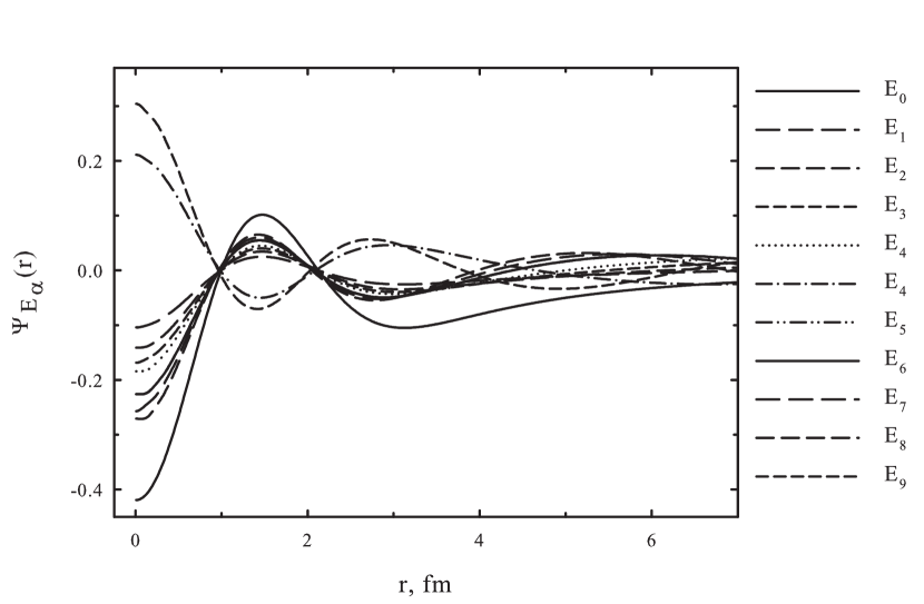
Figure 4: Coordinate wave functions of 10 lowest $0^{+}$ states in ${}^{8}Be$.

In Figure 5 we compare the coordinate wave functions of the ground states in ${}^{6}Li$, ${}^{7}Li$, ${}^{7}Be$ and ${}^{8}Be$ (BS). The wave functions of ${}^{7}Li$ and ${}^{7}Be$ are indistinguishable in this Figure, despite that the energy difference of the bound states is 0.84 MeV.

To demonstrate whether our basis of cluster functions is large enough to provide correct results, in Figure 5 we also display an asymptotic behavior of the wave functions. One can see that the wave functions are decreased as $\exp\left\{-\kappa q\right\}/q$ at large values of $q$. The order of the curves depends on the bound state energy: the smaller is the energy, the lower is the corresponding curve.

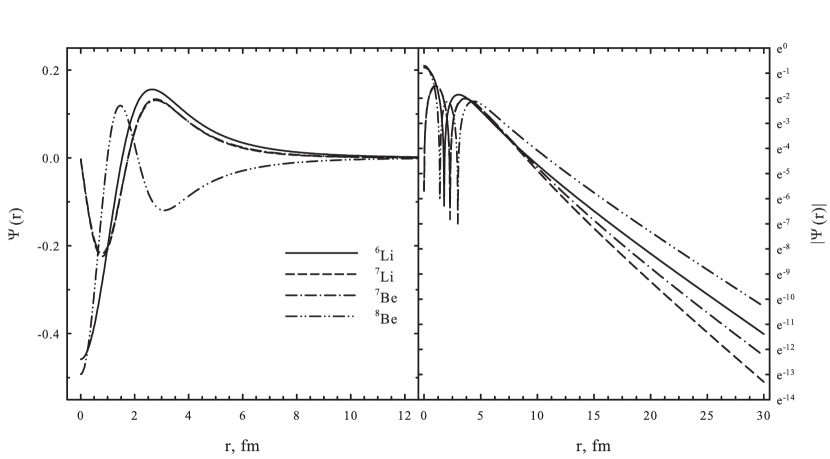
Figure 5: Wave functions of the ground state of ${}^{6}Li$, ${}^{7}Li$, ${}^{7}Be$ and ${}^{8}Be$ in coordinate space. A short range behavior is shown on the left-hand side, while an asymptotic behavior is demonstrated on the right-hand side of the Figure.

6.1 Phase portrait of bound states

Now we turn our attention to the phase portraits of bound states of the two-cluster systems.  In Figures 6, 7 we display the phase portraits of the ${}^{7}Li$ and ${}^{7}Be$ bound states. The phase portrait for the ${}^{6}Li$ ground state was shown in our previous publication [16]. The general feature of these figures is that the two-cluster system is concentrated in a rather narrow region of the phase space, despite the fact that some bound states are weakly bound ones. As was expected, the more dispersed is a state in the coordinate space, the more compact it is in the momentum space. And vise versa. It is interesting to note that a maximum of the density distributions in the phase space of the bound states lies at $\eta\approx 1.0$ and $3.5\leq\xi\leq 4$. The above-mentioned value of $\eta$ is noticeable differs from the dimensionless momentum $k$ (which for the deepest bound state in ${}^{7}Li$ equals $k$=0.46). In our opinion, this indicates that the shape of the density distribution for a bound state has a pure quantum character.

As we see from Fig. 5, the wave functions and thus the density distributions of the ground states in the coordinate space have nodes. There are also nodes in the momentum space for a wave function of bound states. However, the density distribution of the states in the phase space does not have any node in the range $0<\eta<\infty$ and $0<\xi<\infty$.

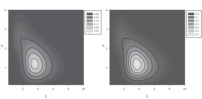
Figure 6: Phase portraits of the $3/2^{-}$ (left) and $1/2^{-}$ (right) bound states in ${}^{7}Li$.

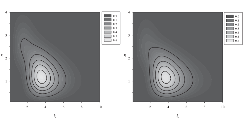
Figure 7: Phase portraits of the $3/2^{-}$ (left) and $1/2^{-}$ (right) bound states in ${}^{7}Be$.

6.2 Phase portrait for resonance states.

There are narrow and broad resonance states in the nuclei of interest. The narrowest resonance state is observed in ${}^{8}Be$. Indeed, the calculated width of the $0^{+}$ resonance state is only 2.40 eV. The broadest resonance state is also observed in ${}^{8}Be$. The width of the $4^{+}$ resonance states exceeds 3.5 MeV. One would expect quite different density distributions and shape of phase portraits for narrow and broad resonance states. This is so, as can be seen from Figures 8, 9, 10, where we display the phase portraits for the resonance states in ${}^{6}Li$, ${}^{7}Li$ and ${}^{7}Be$. Each nucleus is represented by two resonance states, one of which is narrow ($3^{+}$ in ${}^{6}Li$, $7/2^{-}$ in ${}^{7}Li$ and ${}^{7}Be$)  and the other is broad ($2^{+}$ in ${}^{6}Li$, $5/2^{-}$ in ${}^{7}Li$ and ${}^{7}Be$). When we are saying ”a narrow resonance state” or ”a broad resonance state”, we mean not only the absolute value of the resonance width, but also the value of $\Gamma/E$. For narrow resonance states this ratio is below 0.067, and for broad resonance states it exceeds 0.34.  For the narrowest $0^{+}$ resonance state in ${}^{8}Be$, the ratio $\Gamma/E\approx 3\cdot 10^{-5}$.

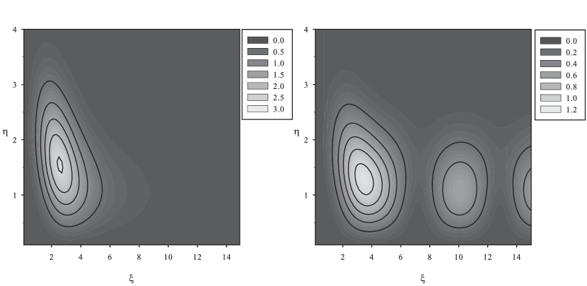
Figure 8: Phase portraits of the $3^{+}$ (left) and $2^{+}$ (right) resonance states in ${}^{6}Li$.

There is a strong resemblance between narrow resonance states and bound states. Both of them realize themselves in a compact area of the phase space.

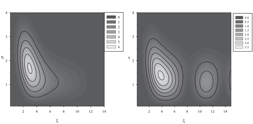
Figure 9: Phase portraits of the $\frac{7}{2}^{-}$ and $\frac{5}{2}^{-}$ resonance states in ${}^{7}Li$.

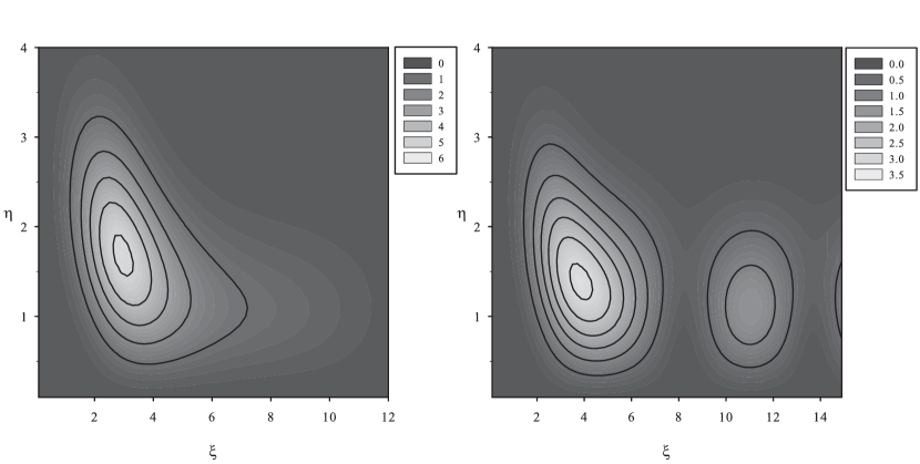
Figure 10: Phase portraits of the $\frac{7}{2}^{-}$ and $\frac{5}{2}^{-}$ resonance states in ${}^{7}Be$.

As for the broad resonance states, they have a principal maximum at relatively small values of coordinates $\xi$ and momenta $\eta$. Besides, they also have many regular maxima at a fixed value of $\eta$, but different values of $\xi$. This structure reflects an oscillatory behavior of the coordinate wave function and $\delta$-like behavior of the wave function in the momentum space.

In Figure 11 we compare phase portraits of the $0^{+}$ ”ground” state in ${}^{8}Be$, obtained with and without the Coulomb interaction (RS and BS calculations). The energy of the resonance state is 0.0818 MeV above the $\alpha+\alpha$ threshold, while the energy of the bound state is -1.3529 MeV bellow the threshold.

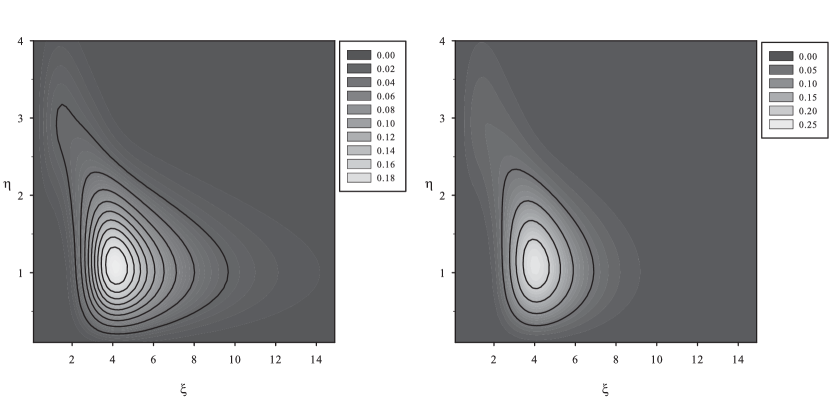
Figure 11: Phase portraits of $0^{+}$ resonance (left) and bound (right) states in ${}^{8}Be$.

One can see, that the phase portraits of resonance and bound states are quite similar. This similarity can be attributed to the fact that in the internal region, where interaction between clusters is strong, wave functions have very close behavior. The asymptotic part of these functions are totally different. For a bound state, the function $\psi\left(q\right)$ exponentially decreases  (24), while it slowly decreases (26) for a resonance state. Thus, the asymptotic part of wave functions gives a small contribution to a density distribution in the Fock-Bargmann space. To prove that in the internal region wave function of resonance and bound state are similar, we display  in Figures 12 the density distributions in the coordinate and momentum representations. Indeed, these figures show that there is small difference between the wave functions or density distributions of the bound and resonance states in ${}^{8}Be$. Maximum of density distributions is approximately in the same point of the coordinate space. However, maxima of density distribution of a BS and RS in the momentum space lie at different values of momentum $p$, which connected with different energies of the resonance state (0.0809 MeV) and bound state (-1.3529 MeV). Since the wave function of the bound state is more compact in the coordinate space than the resonance one, it is more dispersed in the momentum space.

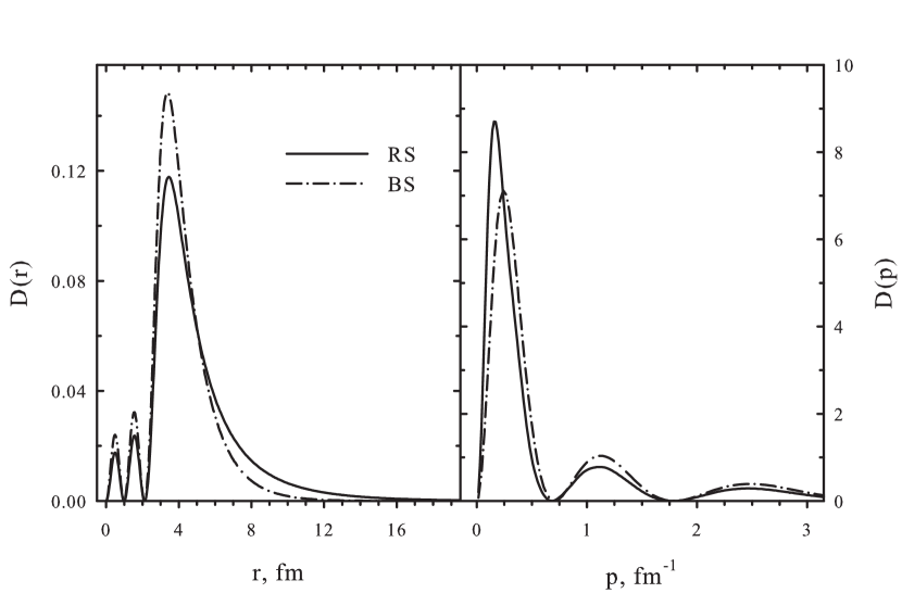
Figure 12: Density distributions of the $0^{+}$ resonance and bound states in ${}^{8}Be$ in coordinate (left) and momentum (right) spaces.

It is interesting to compare a density distribution in the phase space with density distributions in the coordinate and momentum spaces.  For this aim, we find a point in the phase space ($\xi_{\max}$, $\eta_{\max}$) such that the density distributions has maximum. And then, we calculate the density distributions $D\left(\xi,\eta_{\max}\right)$ and $D\left(\xi_{\max},\eta\right)$. Thus from a large number of trajectories, we selected only two of them, the first one is  with a fixed momentum $\eta_{\max}$, the second one is with a fixed coordinate $\xi$. The first trajectory we compare with the density distribution in the coordinate space $D\left(r\right)$, and the second trajectory is compared with the density distribution in the momentum space $D\left(p\right)$. These results are presented in Figure 13. One can see, that the density distributions $D\left(\xi,\eta_{\max}\right)$ and $D\left(r\right)$ are quite close to each other, they have maximum approximately at the same point $\xi\simeq r$. There are more differences in behavior of the density distributions $D\left(\xi_{\max},\eta\right)$ and $D\left(p\right)$. Maximum of $D\left(p\right)$ is shifted to smaller values of $p$, as compared to the function $D\left(\xi_{\max},\eta\right)$. Such relation between $D\left(\xi,\eta_{\max}\right)$ and $D\left(r\right)$, $D\left(\xi_{\max},\eta\right)$ and $D\left(p\right)$ is also observed for bound and resonance states of other nuclei.

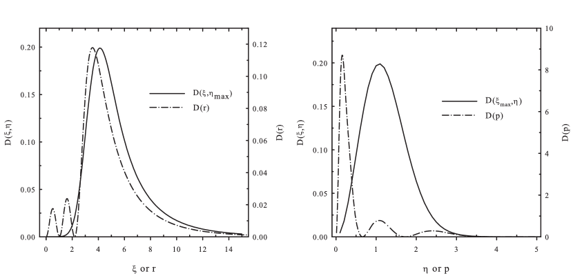
Figure 13: Density distributions in phase space and in coordinate and momentum representations for $0^{+}$ resonance state in ${}^{8}Be$. See more detail in text.

By closing this section, in Figure 14 we demonstrate the phase portraits for the broad $2^{+}$ and $4^{+}$ resonance states. One can see that the oscillations of the density distribution along the axis $\xi$ is more frequent for the $4^{+}$ resonance state than for the $2^{+}$ resonance state. This is expected feature of the density distribution, because the energy of the $4^{+}$ resonance state exceeds the energy of the $2^{+}$ resonance state by a factor of 8. Both resonance states reveal strong quantum effects, because they have prominent maximum in the region of small intercluster distances in the phase space.

Figure 14: Phase portraits for the $2^{+}$ (left) and $4^{+}$ (right) resonance states in ${}^{8}Be$.

As with the bound states, a maximum of the density distribution in phase space for the resonance states is also observed at the values of variable $\eta$, which significantly differ from the corresponding value of the dimensionless parameter $k$. To demonstrate this, we consider the resonance states in ${}^{8}Be$. The dimensionless parameter $k$ for ${}^{8}Be$, where the $0^{+}$ resonance state has the smallest energy and the $4^{+}$ resonance state has the largest energy, varies at the range 0.086$\leq k\leq$0.944. However, a maximum of the density distribution for the $4^{+}$ resonance state is achieved at $\eta\approx 1.5$. This value has to be compared with $k=$0.944. For the $0^{+}$ resonance state, the momentum $k$=0.086; and the density distribution peaks at $\eta\approx 1.1$.

6.3 Classical regime

In this subsection, we consider the high energy excited state of the two-cluster systems. So far we considered excited states with the energy less than 10 MeV. Now we will look for the range of energy, where phase portraits have an evident ”classical shape” or where all quantum trajectories approach classical trajectories.

Let us consider the excited $0^{+}$ states of ${}^{8}Be$ with energy $E$=60.21 MeV, Figure 15. This energy corresponds to the dimensionless momentum $k=b\sqrt{\frac{2mE}{\hbar^{2}}}$=2.34. One can see that the maximum of the density distribution is observed for such value of $\eta$ which is very close to the corresponding value of momentum $k$. This means that the classical regime is realized for a relatively small value of the excitation energy of the two-cluster system. Besides, one can see that the density distribution, presented in Figure 15, is similar to that for free motion of a particle with a large value of the momentum $k$ (cf. with Fig. 7 and eq. (11)). It is important to underline, that the classical regime becomes valid for a moderate value of the coordinate $\xi$.

The correspondence between a quantum density distribution and its classical limit is observed for other values of the total angular momenta in the ${}^{8}Be$ and for all angular momenta in other nuclei as well. The larger is the energy of the excited state, the closer is the density distribution to the classical trajectory.

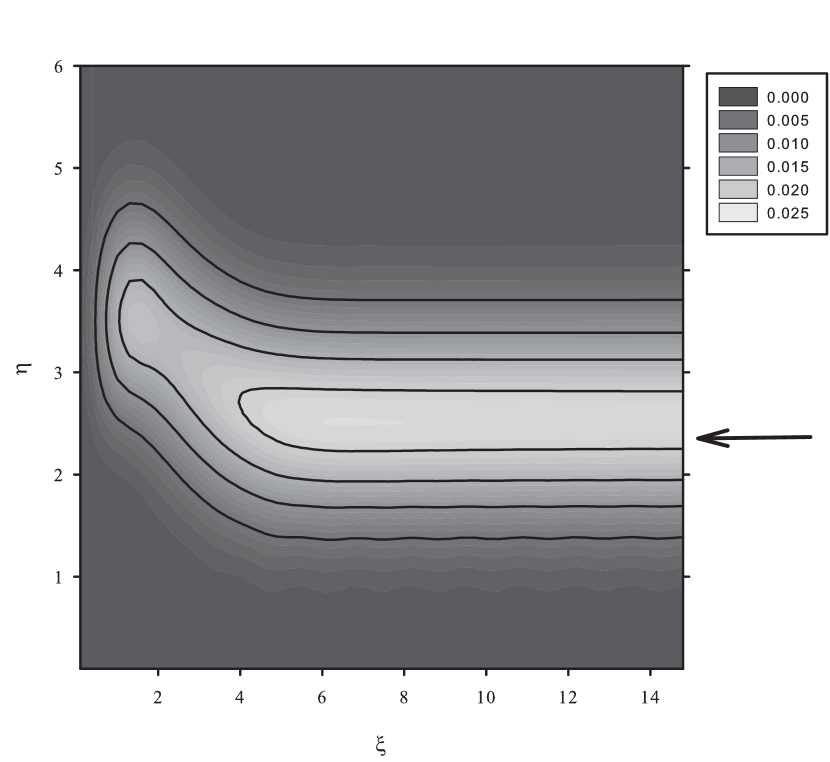
Figure 15: Phase portrait for $0^{+}$ excited state in ${}^{8}Be$ with energy $E$=60.21 MeV and dimensionless momentum $k$=2.34 (this value is indicated by arrow).

7 Conclusions

We have studied the trajectories of two-cluster nuclear systems in phase space. The Bargmann-Segal transformation has been used to map wave functions of two-cluster systems in the coordinate space into the Fock-Bargmann space.  The two-cluster systems have been studied within a microscopic model which makes use of a full set of oscillator functions to expand a wave function of relative motion of interacting clusters. The dominant two-cluster partition of each nuclei was taken into consideration. The input parameters of the model and nucleon-nucleon potential were selected to optimize description of the internal structure of clusters and to reproduce position of the ground state with respect to the two-cluster threshold. We have considered a wide range of excitation energies of compound systems, but special attention was devoted to the bound and resonance states. It was shown that bound states and narrow resonance states realize themselves in a very compact area of the phase space. Phase portraits of the excited states with large value of the energy have a maximal value along the line which coincides with a classical trajectory.

We have also considered two model problems, a harmonic oscillator and free motion in a three-dimensional case, which helped us to understand the dynamics of real physical systems in the phase space.

8 Acknowledgment

This work was supported in part by the Program of Fundamental Research of the Physics and Astronomy Department of the National Academy of Sciences of Ukraine.

References

- [1] K. Takahashi, Wigner and Husimi Functions in Quantum Mechanics, J. Phys. Soc. Jpn. 55 (1986) 762. doi:10.1143/JPSJ.55.762.
- [2] C. K. Zachos, D. B. Fairlie, and T. L. Curtright, Quantum Mechanics in Phase Space, World Scientific, Singapore, 2005.
- [3] K. B. Møller, Comment on phase-space representation of quantum state vectors, J. Math. Phys. 40 (1999) 2531–2535. doi:10.1063/1.532881.
- [4] G. Torres-Vega, J. H. Frederick, A quantum mechanical representation in phase space, J. Chem. Phys. 98 (1993) 3103–3120. doi:10.1063/1.464085.
- [5] K. B. Møller, T. G. Jørgensen, G. Torres-Vega, On coherent-state representations of quantum mechanics: Wave mechanics in phase space, J. Chem. Phys. 106 (1997) 7228–7240. doi:10.1063/1.473684.
- [6] G. Torres-Vega, J. H. Frederick, Quantum mechanics in phase space: New approaches to the correspondence principle, J. Chem. Phys. 93 (1990) 8862–8874. doi:10.1063/1.459225.
- [7] V. Fock, Verallgemeinerung und Lösung der Diracschen statistischen Gleichung, Zeit. Phys. 49 (1928) 339–357. doi:10.1007/BF01337923.
- [8] V. Bargmann, Irreducible unitary representations of the Lorentz group, Ann. Math. 48 (1947) 568–640. doi:10.2307/1969129.
- [9] A. Perelomov, Generalized coherent states and their applications, Berlin, Springer, 1986.
- [10] Y. Kanada-En’yo, M. Kimura, H. Horiuchi, Antisymmetrized Molecular Dynamics: a new insight into the structure of nuclei, C. R. Physique 4 (2003) 497–520. doi:10.1016/S1631-0705(03)00062-8.
- [11] Y. Kanada-En’yo, M. Kimura, A. Ono, Antisymmetrized molecular dynamics and its applications to cluster phenomena, Prog. Theor. Exp. Phys. 2012 (1) (2012) 010000. arXiv:1202.1864, doi:10.1093/ptep/pts001.
- [12] H. Feldmeier, J. Schnack, Molecular dynamics for fermions, Rev. Mod. Phys. 72 (2000) 655–688. arXiv:cond-mat/0001207, doi:10.1103/RevModPhys.72.655.
- [13] T. Neff, H. Feldmeier, Cluster structures within Fermionic Molecular Dynamics, Nucl. Phys. A 738 (2004) 357–361. arXiv:arXiv:nucl-th/0312130, doi:10.1016/j.nuclphysa.2004.04.061.
- [14] J. A. Wheeler, Molecular Viewpoints in Nuclear Structure, Phys. Rev. 52 (1937) 1083–1106. doi:10.1103/PhysRev.52.1083.
- [15] G. Filippov, Y. Lashko, Structure of Light Neutron-Rich Nuclei and Nuclear Reactions Involving These Nuclei, Phys. Part. Nucl. 36 (6) (2005) 714–739.
- [16] Y. A. Lashko, G. F. Filippov, V. S. Vasilevsky, M. D. Soloha-Krymchak, Phase Portraits of Quantum Systems, Few-Body Syst. 55 (8-10) (2014) 817–820. doi:10.1007/s00601-013-0760-8.
- [17] K. Wildermuth, Y. Tang, A unified theory of the nucleus, Vieweg Verlag, Braunschweig, 1977.
- [18] G. F. Filippov, I. P. Okhrimenko, Use of an oscillator basis for solving continuum problems, Sov. J. Nucl. Phys. 32 (1981) 480–484.
- [19] G. F. Filippov, On taking into account correct asymptotic behavior in oscillator-basis expansions, Sov. J. Nucl. Phys. 33 (1981) 488–489.
- [20] G. F. Filippov, V. S. Vasilevsky, L. L. Chopovsky, Solution of problems in the microscopic theory of the nucleus using the technique of generalized coherent states, Sov. J. Part. and Nucl. 16 (1985) 153–177.
- [21] D. R. Thompson, M. LeMere, Y. C. Tang, Systematic investigation of scattering problems with the resonating-group method, Nucl. Phys. A286 (1) (1977) 53–66. doi:10.1016/0375-9474(77)90007-0.
- [22] I. Reichstein, Y. C. Tang, Study of N + system with the resonating-group method, Nucl. Phys. A 158 (1970) 529–545. doi:10.1016/0375-9474(70)90201-0.
- [23] D. R. Tilley, C. M. Cheves, J. L. Godwin, G. M. Hale, H. M. Hofmann, J. H. Kelley, C. G. Sheu, H. R. Weller, Energy levels of light nuclei =5, 6, 7, Nucl. Phys. A 708 (2002) 3–163. doi:10.1016/S0375-9474(02)00597-3.
- [24] D. R. Tilley, J. H. Kelley, J. L. Godwin, D. J. Millener, J. E. Purcell, C. G. Sheu, H. R. Weller, Energy levels of light nuclei =8, 9, 10, Nucl. Phys. A 745 (2004) 155–362. doi:10.1016/j.nuclphysa.2004.09.059.
- [25] S. Saito, Interaction between Clusters and Pauli Principle, Prog. Theor. Phys. 41 (3) (1969) 705–722. doi:10.1143/PTP.41.705.
- [26] S. Saito, Theory of Resonating Group Method and Generator Coordinate Method, and Orthogonality Condition Model, Prog. Theor. Phys. Suppl. 62 (1977) 11–89. doi:10.1143/PTPS.62.11.