Generation of Bell, W and GHZ states via exceptional points in non-Hermitian quantum spin systems

Abstract

We study quantum phase transitions in non-Hermitian XY and transverse-field Ising spin chains, in which the non-Hermiticity arises from the imaginary magnetic field. Analytical and numerical results show that at exceptional points, coalescing eigenstates in these models close to W, distant Bell and GHZ states, which can be steady states in dynamical preparation scheme proposed by T. D. Lee et. al. (Phys. Rev. Lett. 113, 250401 (2014)). Selecting proper initial states, numerical simulations demonstrate the time evolution process to the target states with high fidelity.

I Introduction

Quantum phase transition can occur in a finite non-Hermitian system, associating parity-time ($\mathcal{PT}$) reversal or other type of symmetry breaking. At the transition point as referred to exceptional point (EP), a pair of eigen states coalesces into a single state. Many finite-sized discrete systems have been investigated, including tight-binding models, quantum spin chains, and complex crystal.

These features are different from that of quantum phase transition in infinite Hermitian system. Recently, critical behavior of non-Hermitian system has been employed to generate entangled states in a dynamical process and the corresponding experimental protocol is also proposed Tony1 ; Tony2 . According to the non-Hermitian quantum theory Bender ; Ann ; JMP1 ; JPA1 ; PRL1 ; JMP2 ; JPA3 ; JPA5 , a pseudo-Hermitian system has real eigenvalues or conjugate pair complex eigenvalues. Considering the simplest case, there is only a single pair of eigenstates breaking the symmetry of the Hamiltonian, with conjugate complex eigenvalues. A seed state is an initial state consisting of various eigenstates with eigenvalues with zero, positive and negative imaginary parts, respectively. As time evolution, the amplitude of the state with positive imaginary part in its eigenvalues will increase exponentially and suppress that of other components. The target is the final steady state and expected to have peculiar features for quantum computation processing and other applications. It is important to construct a simple Hamiltonian which is suitable for experimental implementation: to prepare desirable quantum states with high fidelity.

In quantum information science, it is a crucial problem to develop techniques for generating entanglement among stationary qubits, which plays a central role in applications Ekert ; Deutsch ; Bennett . Bell states are specific maximally entangled quantum states of two qubits. For many-qubit system, there are two typical multipartite entangled states, Greenberger-Horne-Zeilinger (GHZ) and W states, which are usually referred to as maximal entanglement. Multipartite entanglement has been recognized as a powerful resource in quantum information processing and communication. Numerous protocols for the preparation of such states have been proposed Cirac ; Gerry ; Hagley ; Cabrillo ; Bose ; Lange ; Rauschenbeutel ; Zheng ; Feng ; Simon ; Zou ; Duan ; SongJ ; Su ; SongHS ; LiY PRA ; Jin2 .

In this paper, we consider whether it is possible to use non-Hermitian systems to generate a W, distant Bell and GHZ states via the dynamical process near EPs. We introduce a non-Hermitian $XY$ and a transverse-field Ising spin chains to demonstrate the schemes. Numerical simulations show that the target states can be obtained with high fidelity by the time evolutions of selecting proper initial states.

The remainder of this paper is organized as follows. In Sec. II, we present a non-Hermitian $XY$ spin model and solutions. Secs. III, IV and V are devoted to the schemes of preparing W, Bell and GHZ states, respectively. Finally, we present a summary and discussion in Sec. VI.

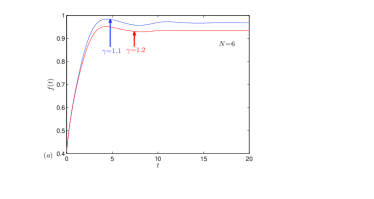
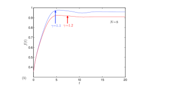
Figure 1: (Color online) Plots of the fidelity $f\left(t\right)$ for preparing W state, as a function of time for the systems with $N=6$ (a) and $8$ (b). The times are dimensionless and in units of $1$. We see that the fidelities converge to constants in exponential manner and the converging fidelities become higher as $\gamma$ closes to $1$, while the converging times get longer. The obtained results are not sensitive to the size $N$, which is quite different from the situations for the productions of Bell and GHZ states.

II $XY$ Spin chain

We consider a non-Hermitian $XY$ spin model

$$H_{\text{chain}} = \frac{1}{2}\sum_{l=1}^{N-1}\left(\sigma_{l}^{x}\sigma_{l+1}^{x}+\sigma_{l}^{y}\sigma_{l+1}^{y}\right)+\text{{H.c.}}$$ (1)

$$\left(V+i\gamma\right)\sigma_{1}^{z}+\left(V-i\gamma\right)\sigma_{N}^{z},$$

on an $N$-site chain, where $\sigma_{l}^{\alpha}$ ($\alpha=x,y,z$) is Pauli matrix. In the case of $\gamma=0$, it is reduced to a Hermitian model with $\mathcal{P}$ symmetry. Here the parity operator $\mathcal{P}$ is given by $\mathcal{P}\sigma_{l}^{\alpha}\mathcal{P}^{-1}=\sigma_{\bar{l}}^{\alpha}$ with $\bar{l}=(N+1-l)$. In the case of nonzero $\gamma$, the $\mathcal{P}$ symmetry is broken, but $\mathcal{PT}$ is still symmetric, where $\mathcal{T}$ is a time reversal operator $\mathcal{T}i\mathcal{T}^{-1}=-i$.

We note that

$$\left[J_{z},H_{\text{chain}}\right]=0,$$ (2)

where $J_{\alpha}=\sum_{l=1}^{N}\sigma_{l}^{\alpha}$ is a total spin operator. This means that $H_{\text{chain}}$ can be diagonalized in each invariant subspace.In this paper, we only concern the issue in the subspace with $J_{z}=N-1$ and $N=$even. In this invariant subspace, the wave function has the form

$$\left|\phi\right\rangle=\sum_{l=1}^{N}f_{l}\sigma_{l}^{+}\left|\Downarrow\right\rangle,$$ (3)

where $\left|\Downarrow\right\rangle$ is a saturated ferromagnetic state $\left|\Downarrow\right\rangle=\prod_{l=1}^{N}\left|\downarrow\right\rangle$. Then we get an equivalent Hamiltonian

$$H_{\text{eq}} = \sum_{l=1}^{N-1}\left|l\right\rangle\left\langle l+1\right|+\text{H.c.}$$ (4)

$$+\left(V+i\gamma\right)\left|1\right\rangle\left\langle 1\right|+\left(V-i\gamma\right)\left|N\right\rangle\left\langle N\right|,$$

where the position state at $l$th site is $\left|l\right\rangle\equiv\sigma_{l}^{+}\left|\Downarrow\right\rangle$. The eigen problem of the equivalent Hamiltonian is given in Appendix. In the following, we will discuss the schemes for the preparation of W and Bell states based on the Hamiltonian $H_{\text{eq}}$.

III W state

In the situation $V=0$, the Hamiltonian $H_{\text{eq}}$ is reduced to

$$H_{\text{W}}=\sum_{l=1}^{N-1}\left|l\right\rangle\left\langle l+1\right|+\text{H.c.}+i\gamma\left|1\right\rangle\left\langle 1\right|-i\gamma\left|N\right\rangle\left\langle N\right|.$$ (5)

The exact solution in the Appendix suggests us to consider the state

$$\left|\text{W}\right\rangle=\frac{1}{\sqrt{N}}\sum_{l=1}^{N}\left(-i\right)^{l}\sigma_{l}^{+}\left|\Downarrow\right\rangle=\frac{1}{\sqrt{N}}\sum_{l=1}^{N}\left(-i\right)^{l}\left|l\right\rangle,$$ (6)

which represents a single-magnon spin wave with wave vector $\pi/2$. It is a W state under a local transformation $\left(-i\right)^{l}\sigma_{l}^{+}\rightarrow\sigma_{l}^{+}$, which does not reduce its properties in quantum information processing. A straightforward derivation shows that the state $\left|\text{W}\right\rangle$ is an eigenstate of the Hamiltonian $H_{\text{W}}$ at $\gamma=\gamma_{c}=1$, i.e.,

$$H_{\text{W}}\left(\gamma_{c}\right)\left|\text{W}\right\rangle=0\left|\text{W}\right\rangle.$$ (7)

Then, we will show that $\left|\text{W}\right\rangle$ is a special eigenstate of $H_{\text{W}}\left(\gamma_{c}\right)$. For the corresponding conjugate Hamiltonian $H_{\text{W}}^{{\dagger}}\left(\gamma_{c}\right)$, we have

$$H_{\text{W}}^{{\dagger}}\left(\gamma_{c}\right)\left|\mathcal{W}\right\rangle=0\left|\mathcal{W}\right\rangle,$$ (8)

where

$$\left|\mathcal{W}\right\rangle=\frac{1}{\sqrt{N}}\sum_{l=1}^{N}i^{l}\sigma_{l}^{+}\left|\Downarrow\right\rangle$$ (9)

It is easy to find that

$$\langle\mathcal{W}\left|\text{W}\right\rangle=0,$$ (10)

which indicates that $H_{\text{W}}$ has an EP at $\gamma_{c}$ and the W state is the coalescent state at the transition point. In the Appendix, this result is confirmed by an exact Bethe Ansatz analysis.

We investigate the scheme of selecting the $\left|\text{W}\right\rangle$ state by a dynamic process. From the Appendix or the previous work Jin1 , we find that the complex conjugate pair of energies is $\pm i2J\sinh\kappa$ for small $\kappa$, where real number $\kappa$ obeys the equation

$$\gamma^{2}\sinh[\left(N-1\right)\kappa]=\sinh[\left(N+1\right)\kappa].$$ (11)

We note that the value of $\gamma$ determines the gap between the complex conjugate pair of energies, or the converging time. The initial state is taken as $\left|\psi\left(0\right)\right\rangle=\left|1\right\rangle$, the evolved state $\left|\psi\left(t\right)\right\rangle$ is expected to close the target state for sufficient long time. We employ the fidelity

$$f\left(t\right)=\left|\left\langle\text{W}\right|\widetilde{\psi}\left(t\right)\rangle\right|,$$ (12)

to characterize the efficiency of the scheme. Here $\left|\widetilde{\psi}\left(t\right)\right\rangle$ is the Dirac normalized state of $\left|\psi\left(t\right)\right\rangle$ to reduce the increasing norm of $\left|\psi\left(t\right)\right\rangle$. In the limit case of $\gamma\rightarrow 1$, we will have $f\left(t\right)\rightarrow 1$ as $t\rightarrow\infty$. For finite $\gamma$, the time evolution of the state is computed by numerical diagonalization in the broken symmetric region. In order to quantitatively evaluate the fidelity and demonstrate the proposed scheme, we simulate the dynamic processes of the W state preparation. To illustrate the process, we plot the fidelities as functions of time for systems with $N=6$ and $8$ in Fig. 1. It shows that the fidelities converges to a steady value exponentially fast. Smaller $\gamma$ (approaches to $1$) can enhance the fidelity, while the converging time becomes longer. Moreover, we find that the converging times for two cases are not so sensitive to the size $N$, which is quite different from that in following two schemes for preparing distant Bell and GHZ states. This is because of the fact that the phase boundary is always at $\gamma=1$ for any even $N$. Then such a scheme is more efficient for a W-state production.

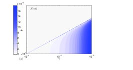
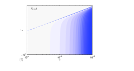
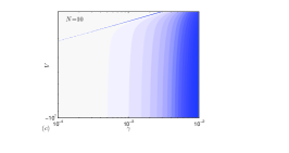
Figure 2: (Color online) Phase diagram of non-Hermitian Hamiltonian in Eq. (4). The color contour map represents the magnitude of the imaginary part of conjugate-pair energy levels for $N=6$, $8$ and $10$, obtained by exact diagonalization. The white area indicates the region where the spectrum is entirely real. The dot line is the plot of function in Eq. (49), indicating the exact phase boundary. We see that all three boundaries are in line shape with different slopes in the logarithm scales. This property can be explained by perturbation approximation.

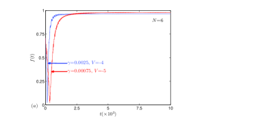
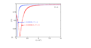
Figure 3: (Color online) Plots of the fidelity $f\left(t\right)$ for preparing Bell state, as a function of time for the systems with $N=6$ (a) and $8$ (b). The times are dimensionless and in units of $10^{3}$ and $10^{4}$, respectively. We see that the converging fidelities approach to $1$, getting higher as increasing of $V$ and longer time. The time scale of (b) is over ten times longer than that of (a), which indicates the difficulty of preparing long-distance Bell state.

IV Bell state

In the situation $\left|V\right|>2$, the exact solution in the Appendix shows that two bound states are formed, in which the probability mainly distributes around two ending sites. The phase diagram has been obtained as Eq. (49) in the Appendix, which is the base of the scheme for preparing Bell state. According to the Bethe Ansatz result, there is a conjugate complex pair of energy levels in the broken $\mathcal{PT}$ symmetric region. The magnitude of the imaginary part of the eigen energy $\left|\text{Im}\varepsilon\right|$ is also an indicator of the phase boundary and determines the converging speed of the scheme. For illustrating this point, we plot $\left|\text{Im}\varepsilon\right|$ as a function of $V$ and $\gamma$ for the systems with $N=6$, $8$ and $10$ in Fig. 2. The corresponding exact boundary from Eq. (49) is plotted as well. We find that they accord with each other and the boundary appears as a linear line with $N$-dependent slope in the logarithm scales. We will see that the profile of the phase diagram directly determines the efficiency of the scheme in the following investigation.

In order to understand a clear physical picture of the exact solution, we use the perturbation method to simplify the Hamiltonian $H_{\text{eq}}$ in large $V$ limit. Although the perturbation theory for non-Hermitian Hamiltonian has not been well established, the following result will show that the corresponding approximation is technically sound by the comparison with the exact solution. We rewrite the Hamiltonian $H_{\text{eq}}$ in the form

$$H_{\text{eq}} = H_{\text{0}}+H^{\prime},$$ (13)

$$H_{\text{0}} = \sum_{l=2}^{N-2}\left|l\right\rangle\left\langle l+1\right|+\text{H.c.}$$ (14)

$$+\left(V+i\gamma\right)\left|1\right\rangle\left\langle 1\right|+\left(V-i\gamma\right)\left|N\right\rangle\left\langle N\right|,$$

$$H^{\prime} = \left|1\right\rangle\left\langle 2\right|+\left|N-1\right\rangle\left\langle N\right|+\text{H.c.,}$$ (15)

where the eigen states of $H_{\text{0}}$ can be easily obtained as $\{\left|1\right\rangle$, $\left|N\right\rangle$, $\sum_{j=2}^{N-1}\sqrt{\frac{2}{N-1}}\sin[\frac{\left(n-1\right)j\pi}{N-1}]\left|N\right\rangle$; $n\in$ $\left[2,N-1\right]\}$ with corresponding energy $\{V+i\gamma$, $V-i\gamma$, $2\cos[\frac{\left(n-1\right)\pi}{N-1}]$; $n\in$ $\left[2,N-1\right]\}$. This set of eigen states has a special feature that they can construct a complete set under the Dirac inner product, even $H_{\text{0}}$ is a non-Hermitian Hamiltonian. Then the effective Hamiltonian for two bound states can be obtained as

$$H_{\text{eff}} = \lambda_{\text{eff}}\left|1\right\rangle\left\langle N\right|+\text{H.c.}+(V+V_{\text{eff}}+i\gamma)\left|1\right\rangle\left\langle 1\right|$$ (16)

$$+(V+V_{\text{eff}}-i\gamma)\left|N\right\rangle\left\langle N\right|,$$

in the case of $\left|V\right|\gg 1$, the model above is a simple two-site model and easily solvable. Here the effective potential is

$$V_{\text{eff}}=\frac{2}{N-1}\sum_{n=2}^{N-1}\frac{\sin^{2}\phi_{n}}{V-2\cos\phi_{n}}\approx\frac{1}{V},$$ (17)

and the effective coupling is

$$\lambda_{\text{eff}} = \frac{2}{N-1}\sum_{n=2}^{N-1}\frac{\sin\phi_{n}\sin[\left(N-2\right)\phi_{n}]}{V-2\cos\phi_{n}}$$ (18)

$$\approx \frac{\Omega}{V^{2}},$$

where parameters $\Omega$, $\phi_{n}$ and $\theta$ are $N$ dependent functions

$$\Omega = \frac{\cos\left[\left(N-4\right)\pi/2\right]\sin[\left(N-4\right)\left(N-2\right)\theta]}{\left(N-1\right)\sin[\left(N-4\right)\theta]}$$ (19)

$$-\frac{\left(-1\right)^{N/2}\sin[\left(N-2\right)N\theta]}{\left(N-1\right)\sin(N\theta)},$$

$$\phi_{n} = 2\left(n-1\right)\theta$$ (20)

$$\theta = \frac{\pi}{2\left(N-1\right)}.$$ (21)

The eigen states of $H_{\text{eff}}$ are

$$(i\gamma\pm\sqrt{\lambda_{\text{eff}}^{2}-\gamma^{2}})\left|1\right\rangle+\lambda_{\text{eff}}\left|N\right\rangle,$$ (22)

with eigenvalues: $\pm\sqrt{\lambda_{\text{eff}}^{2}-\gamma^{2}}+V+V_{\text{eff}}$. At the EP, $\lambda_{\text{eff}}^{2}=\gamma_{c}^{2}$, the coalescent state is

$$i\gamma_{c}\left|1\right\rangle+\lambda_{\text{eff}}\left|N\right\rangle,$$ (23)

with energy

$$\varepsilon_{c}=V+V_{\text{{eff}}}\approx V+\frac{1}{V},$$ (24)

which is in agreement with the approximate expression Eq. (52) in the Appendix. Then the boundary has the form

$$\ln\left|\gamma\right|+2\ln\left|V\right|=\ln\left|\Omega\right|,$$ (25)

in the logarithm scales, indicating a linear phase boundary with a fixed slope. This is qualitatively in agreement with the numerical results in Fig. 2 obtained by the exact solution, where the slopes of the boundary are $N$ dependent.

Based on the phase boundary, one can prepare the target state in the vicinity of the EPs via dynamic process. The target state is a Bell state, expressed as

$$\left|\text{Bell}\right\rangle=\frac{1}{\sqrt{2}}\left(\left|1\right\rangle-i\left|N\right\rangle\right).$$ (26)

The initial state is taken as $\left|\psi\left(0\right)\right\rangle=\left|1\right\rangle$, the evolved state $\left|\psi\left(t\right)\right\rangle$ is expected to close the target state for sufficient long time. We employ the fidelity

$$f\left(t\right)=\left|\left\langle\text{Bell}\right|\widetilde{\psi}\left(t\right)\rangle\right|,$$ (27)

to characterize the efficiency of the scheme. Here $\left|\widetilde{\psi}\left(t\right)\right\rangle$ is the Dirac normalized state of $\left|\psi\left(t\right)\right\rangle$ to reduce the increasing norm of $\left|\psi\left(t\right)\right\rangle$. The time evolution of the state is computed by numerical diagonalization. For given $N$ and $V$, we numerically search an optimal $\gamma$ to obtain higher fidelity in the broken symmetric region. In order to quantitatively evaluate the fidelity and demonstrate the proposed scheme, we simulate the dynamic processes of the quantum state preparation. To illustrate the process, we plot the fidelities as functions of time for systems with $N=6$ and $8$ in Fig. 3. It shows that the fidelities converges to a steady value exponentially fast. Larger $\left|V\right|$ corresponds to smaller optimal $\gamma$, leading to higher fidelity, but longer converging time. We also find that the converging times for two cases are sensitive to the size $N$. These accord with the phase diagrams in Fig. 2: linear boundary indicates that larger ln$\left|V\right|$ matches smaller ln$\gamma$ and slight change of slopes between ln$\left|V\right|$ and ln$\gamma$ results in drastic change of the converging times.

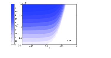
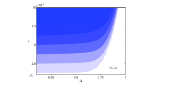
Figure 4: (Color online) Phase diagram of non-Hermitian Hamiltonian in Eq. (29). The color contour map represents the magnitude of the imaginary part of conjugate-pair energy levels for $N=6$ and $8$, obtained by exact diagonalization. The white area indicates the region where the spectrum is entirely real. We see that two boundaries have similar shapes but with a shift.

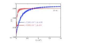
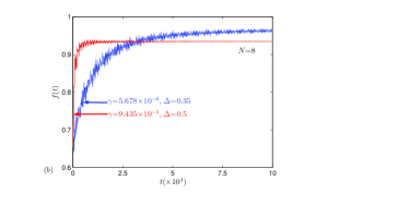
Figure 5: (Color online) Plots of the fidelity $f\left(t\right)$ for preparing GHZ state, as a function of time for the systems with $N=6$ (a) and $8$ (b). The times are dimensionless and in units of $10^{3}$ and $10^{4}$, respectively. We see that the converging fidelities approach to $1$, getting higher as decreasing of $\Delta$ and longer time. The time scale of (b) is over ten times longer than that of (a), which indicates the difficulty of preparing long-distance GHZ state.

V GHZ state

The above conclusion provides a way to prepare a superposition of two distant position states. Such a scheme can be extended to prepare the GHZ state which has the form

$$\left|\text{GHZ}\right\rangle=\left|\Downarrow\right\rangle+\prod_{l=1}^{N}\sigma_{l}^{+}\left|\Downarrow\right\rangle.$$ (28)

States $\left|\Downarrow\right\rangle$ and $\prod_{l=1}^{N}\sigma_{l}^{+}\left|\Downarrow\right\rangle$ can be regarded as two end position states, which are connected by $N$-step operations of operator $\sum_{l=1}^{N}\sigma_{l}^{x}$. This opens a probability to select the GHZ state as a steady state near the EP. We consider a simple and practical model, which is a non-Hermitian Ising model, described by the Hamiltonian

$$H_{\text{{GHZ}}}=-J\sum_{l=1}^{N}\sigma_{l}^{z}\sigma_{l+1}^{z}+i\gamma\sum_{l=1}^{N}\sigma_{l}^{z}+\Delta\sum_{l=1}^{N}\sigma_{l}^{x}.$$ (29)

It is a standard transverse-field Ising model at $\gamma=0$, which can be exactly solved and has been extensively studied in a variety of areas. Recently, theoretical studies of several types of quantum Ising models were extended to the non-Hermitian regime and some peculiar properties were observed Korff ; Castro ; Deguchi ; Giorgi ; Bytsko ; Zhang1 ; Li . In the case of $J=0$, this model is reduced to non-interacting spin-$1/2$ particles with complex magnetic field, which has full real spectrum when $\Delta^{2}\eqslantgtr\gamma^{2}$ Zhang3 . We assume that the phase transition can occur in the case of nonzero $\gamma$ and $J$. Since this model is not solvable, we perform numerical simulation by exact diagonalization.

Similarly as last section, we still employ the magnitude of the imaginary part of the eigen energy $\left|\text{Im}\varepsilon\right|$ as an indicator to characterize the phase boundary. Taking $J=1$, we plot $\left|\text{Im}\varepsilon\right|$ as a function of $V$ and $\gamma$ for the systems with $N=6$ and $8$ in Fig. 4. We find that the phase boundaries of the two cases have the similar profile but with a shift. This will be reflected on the speed of the fidelity convergence.

For a GHZ state preparation, the initial state is taken as $\left|\psi\left(0\right)\right\rangle=\left|1\right\rangle$, the evolved state $\left|\psi\left(t\right)\right\rangle$ is expected to close the target state for sufficient long time. We employ the fidelity

$$f\left(t\right)=\left|\left\langle\text{GHZ}\right|\widetilde{\psi}\left(t\right)\rangle\right|,$$ (30)

to characterize the efficiency of the scheme. Here $\left|\widetilde{\psi}\left(t\right)\right\rangle$ is the Dirac normalized state of $\left|\psi\left(t\right)\right\rangle$ to reduce the increasing norm of $\left|\psi\left(t\right)\right\rangle$. The time evolution of the state is computed by numerical diagonalization. For given $N$ and $V$, we numerically search an optimal $\gamma$ to obtain higher fidelity in the broken symmetric region. In order to quantitatively evaluate the fidelity and demonstrate the proposed scheme, we simulate the dynamic processes of the quantum state preparation. To illustrate the process, we plot the fidelities as functions of time for systems with $N=6$ and $8$ in Fig. 5. The obtained results are similar to the case of Bell-state production at last.

VI Summary

In summary, we presented schemes to generate W, distant Bell and GHZ states by exploiting the quantum phase transitions in non-Hermitian $XY$ and transverse-field Ising spin chains. The phase diagrams for such two models are obtained analytically and numerically, which is crucial for the practical realization of the scheme. Numerical simulations on the dynamics process for state preparation show that the evolved states close to target states in an exponential manner over time. Comparing the dynamical preparation of quantum state via Hermitian system, where the acquired state only emerges within a short time window, this scheme can provide the steady final state. A shortcoming of the scheme is that the production period for Bell and GHZ states increases rapidly as cluster size grows. However, this scheme is more efficient for a W-state production.

*

Appendix A Exact solution of the $H_{\text{eq}}$

In this appendix, we present the exact results for the solutions of following model

$$H_{\text{{eq}}} = \sum_{l=1}^{N-1}\left|l\right\rangle\left\langle l+1\right|+\text{{H.c.}}$$ (31)

$$+\left(V+i\gamma\right)\left|1\right\rangle\left\langle 1\right|+\left(V-i\gamma\right)\left|N\right\rangle\left\langle N\right|,$$

and the EPs in the cases of $V=0$ and $\left|V\right|>2$.

A.1 $V=0$ case

The Bethe Ansatz wave function is in the form

$$\left|k\right\rangle=\sum_{j=1}^{N}\left(A_{k}e^{ikj}+B_{k}e^{-ikj}\right)\left|j\right\rangle,$$ (32)

where $k$ is real number, indicating a scattering state. The Schrodinger equation $H\left|k\right\rangle=\varepsilon_{k}\left|k\right\rangle$ can be written as

$$M\left[\begin{array}[]{c}A_{k}\\ B_{k}\end{array}\right]=0,$$ (33)

where the matrix

$$M = \left[\begin{array}[]{cc}\upsilon_{+}e^{ik}+e^{ik2}&\upsilon_{+}e^{-ik}+e^{-ik2}\\ \upsilon_{-}e^{ikN}+e^{ik\left(N-1\right)}&\upsilon_{-}e^{-ikN}+e^{-ik\left(N-1\right)}\end{array}\right],$$ (36)

$$\upsilon_{\pm} = \pm i\gamma-\varepsilon_{k},$$ (37)

and the real spectrum

$$\varepsilon_{k}=2\cos k.$$ (38)

The existence of solution requires

$$\det\left|M\right|=0,$$ (39)

which leads to the equation

$$F\left(k\right)=\sin\left[k\left(N+1\right)\right]+\gamma^{2}\sin\left[k\left(N-1\right)\right]=0.$$ (40)

The EP $k_{c}$ can be determined by equation

$$F\left(k_{c}\right)=\frac{\partial}{\partial k}F\left(k_{c}\right)=0.$$ (41)

We obtain $k_{c}=\pi/2$ at $\gamma=1$ (see ref. Jin1 ).

A.2 $\left|V\right|>2$ case

In this situation, we are interested in bound states. The corresponding Bethe Ansatz wave function is in the form

$$\left|\kappa\right\rangle=\sum_{j=1}^{N}\left(\alpha_{\kappa}e^{\kappa j}+\beta_{\kappa}e^{-\kappa j}\right)\left|j\right\rangle,$$ (42)

where $\kappa$ is a real number. By the similar procedure, we reach the equation

$$\digamma\left(\kappa_{c}\right)=\frac{\partial}{\partial\kappa}\digamma\left(\kappa_{c}\right)=0,$$ (43)

which determines the location of EPs at energy

$$\epsilon_{\kappa_{c}}=2\cosh\kappa_{c},$$ (44)

where function

$$\digamma\left(\kappa\right) = \sinh\left[\left(N+1\right)\kappa\right]-2V\sinh\left(N\kappa\right)$$ (45)

$$+\left(V^{2}+\gamma^{2}\right)\sinh\left[\left(N-1\right)\kappa\right].$$

From Eq. (43), we have

$$\frac{\left[N\eta_{+}+\eta_{-}\right]\cosh\kappa_{c}-2NV}{\left(N\eta_{-}+\eta_{+}\right)\sinh\kappa_{c}}$$ (46)

$$= \frac{\eta_{-}\sinh\kappa_{c}}{\eta_{+}\cosh\kappa_{c}-2V}=-\tanh\left(N\kappa_{c}\right),$$

where

$$\eta_{\pm}=1\pm V^{2}\pm\gamma^{2}.$$ (47)

The bound state EPs require

$$\left|\epsilon_{\kappa_{c}}\right|>2\left|V\right|.$$ (48)

Such solutions exist when parameters $V$ and $\gamma$ satisfy

$$(c+\sqrt{c^{2}-1})^{2N}=\frac{\eta_{+}c-2V-\eta_{-}\sqrt{c^{2}-1}}{\eta_{+}c-2V+\eta_{-}\sqrt{c^{2}-1}},$$ (49)

which indicates the exact phase boundary and is plotted in Fig. 2 for the cases of $N=6$ and $8$. Here real number $c$ is

$$c=\cosh\kappa=F[1$$

$$+\sqrt{1-\frac{4N\left(\eta_{+}-1\right)\left(N\eta_{-}^{2}+\eta_{+}\eta_{-}+4NV^{2}\right)}{V^{2}\left(2N\eta_{+}+\eta_{-}\right)^{2}}}].$$ (50)

$$F=\frac{V\left(2N\eta_{+}+\eta_{-}\right)}{4N\left(\eta_{+}-1\right)}$$ (51)

In the case of $\left|V\right|\gg 1$, we have

$$c\approx\frac{V}{2}+\frac{1}{2V},$$ (52)

which gives the approximate energy expression $\epsilon_{\kappa}=2\cosh\kappa\approx V+\frac{1}{V}$.

- (1) T. E. Lee, F. Reiter, and N. Moiseyev, Phys. Rev. Lett. 113, 250401 (2014).
- (2) T. E. Lee and C. K. Chan, Phys. Rev. X 4, 041001 (2014).
- (3) C. M. Bender and S. Boettcher, Phys. Rev. Lett. 80, 5243 (1998).
- (4) F. G. Scholtz, H. B. Geyer, and F. J. W. Hahne, Ann. Phys. (NY) 213, 74 (1992).
- (5) C. M. Bender, S. Boettcher, and P. N. Meisinger, J. Math. Phys. 40, 2201 (1999).
- (6) C. M. Bender, D. C. Brody, and H. F. Jones, Phys. Rev. Lett. 89, 270401 (2002).
- (7) P. Dorey, C. Dunning, and R. Tateo, J. Phys. A 34, L391 (2001); J. Phys. A 34, 5679 (2001).
- (8) A. Mostafazadeh, J. Math. Phys. 43, 205 (2002); J. Math. Phys. 43, 2814 (2002); J. Math. Phys. 43, 3944 (2002).
- (9) A. Mostafazadeh and A. Batal, J. Phys. A 36, 7081 (2003); J. Phys. A 37, 11645 (2004).
- (10) H. F. Jones, J. Phys. A 38, 1741 (2005).
- (11) A. K. Ekert, Phys. Rev. Lett. 67, 661 (1991).
- (12) D. Deutsch and R. Jozsa, Proc. R. Soc. London A 439, 553 (1992).
- (13) C. H. Bennett, G. Brassard, C. Crepeau, R. Jozsa, A. Peres, and W. K. Wootters, Phys. Rev. Lett. 70, 1895 (1993).
- (14) J. I. Cirac and P. Zoller, Phys. Rev. A 50, R2799 (1994).
- (15) C. C. Gerry, Phys. Rev. A 53, 2857 (1996).
- (16) E. Hagley, X. Maitre, G. Nogues, C. Wunderlich, M. Brune, J. M. Raimond, and S. Haroche, Phys. Rev. Lett. 79, 1 (1997).
- (17) C. Cabrillo, J. I. Cirac, P. Garcia-Fernandez, and P. Zoller, Phys. Rev. A 59, 1025 (1999).
- (18) S. Bose, P. L. Knight, M. B. Plenio, and V. Vedral, Phys. Rev. Lett. 83, 5158 (1999).
- (19) W. Lange and H. J. Kimble, Phys. Rev. A 61, 063817 (2000).
- (20) A. Rauschenbeutel, G. Nogues, S. Osnaghi, P. Bertet, M. Brune, J. Raimond, and S. Haroche, Science 288, 2024 (2000).
- (21) S. B. Zheng, Phys. Rev. Lett. 87, 230404 (2001).
- (22) X. L. Feng, Z. M. Zhang, X. D. Li, S. Q. Li, S. Q. Gong, and Z. Z. Xu, Phys. Rev. Lett. 90, 217902 (2003).
- (23) C. Simon and W. T. M. Irvine, ibid. 91, 110405 (2003).
- (24) X. B. Zou, K. Pahlke, and W. Mathis, Phys. Rev. A 68, 024302 (2003).
- (25) L. M. Duan and H. J. Kimble, Phys. Rev. Lett. 90, 253601 (2003).
- (26) J. Song, Y. Xia, H. S. Song, J. L. Guo, and J. Nie, Europhys. Lett. 80, 60001 (2007).
- (27) X. Su, A. Tan, X. Jia, J. Zhang, C. Xie, and K. Peng, Phys. Rev. Lett. 98, 070502 (2007).
- (28) Y. Xia, J. Song, and H.S. Song, Appl. Phys. Lett. 92, 021127 (2008).
- (29) Y. Li, T. Shi, B. Chen, Z. Song, C. P. Sun, Phys. Rev. A 71, 022301 (2005); M. X. Huo, Y. Li, Z. Song and C. P. Sun, Europhys. Lett. 84 30004 (2008); S. Yang, Z. Song, and C. P. Sun, Science China Physics, Mechanics & Astronomy Volume: 51 Issue: 1 Pages: 45-55 (2008).
- (30) L. Jin and Z. Song, Phys. Rev. A 79, 042341 (2009).
- (31) L. Jin and Z. Song, Phys. Rev. A 80, 052107 (2009).
- (32) C. Korff and R. A. Weston, J. Phys. A40, 8845—8872 (2007).
- (33) O. A. Castro-Alvaredo and A. Fring, J. Phys. A42, 465211 (2009).
- (34) T. Deguchi. and P. K. Ghosh, J. Phys. A42, 475208 (2009).
- (35) G. L. Giorgi, Phys. Rev. B 82, 052404 (2010).
- (36) A. G. Bytsko, St. Petersburg Math. J. Vol. 22, No. 3, Pages 393–410(2011).
- (37) X. Z. Zhang and Z. Song, Phys. Rev. A 87, 012114 (2013); Phys. Rev. A 88, 042108 (2013).
- (38) C. Li, G. Zhang, X. Z. Zhang, and Z. Song, Phys Rev. A 90, 012103 (2014).
- (39) X. Z. Zhang, L. Jin, and Z. Song, Phys. Rev. A. 85, 012106 (2012).