Polar rotation angle identifies elliptic islands in unsteady dynamical systems

Abstract

We propose rotation inferred from the polar decomposition of the flow gradient as a diagnostic for elliptic (or vortex-type) invariant regions in non-autonomous dynamical systems. We consider here two- and three-dimensional systems, in which polar rotation can be characterized by a single angle. For this polar rotation angle (PRA), we derive explicit formulas using the singular values and vectors of the flow gradient. We find that closed level sets of the PRA reveal elliptic islands in great detail, and singular level sets of the PRA uncover centers of such islands. Both features turn out to be objective (frame-invariant) for two-dimensional systems. We illustrate the diagnostic power of PRA for elliptic structures on several examples.

1 Introduction

Complex dynamical systems exhibit a mixture of chaotic and coherent behavior in their phase space. The latter manifests itself in coherent islands of regular behavior surrounded by a chaotic background flow. The best known classic examples of such islands are formed by Kolmogorov–Arnold-Moser (KAM) tori, composed of quasi-periodic trajectories in Hamiltonian systems [see, e.g., 1, 2]. Outside elliptic regions filled by such tori, chaotic trajectories dominate the dynamics.

Even more intriguing is the existence of similar elliptic islands in turbulent fluid flow, as broadly confirmed by experiments and numerical simulations [see, e.g., 3, 4]. Just as KAM islands, coherent vortices capture trajectories and keep them out of chaotic mixing zones. Unlike KAM tori, however, coherent vortices are composed of trajectories that are generally not recurrent in any frame. During their finite time of existence, these coherent vortices traverse without filamentation but also without displaying any particular periodic or quasiperiodic pattern. Still, we generally refer to such regions here as elliptic, as they mimic the dynamic role of elliptic islands occupied by classic KAM tori.

Eulerian approaches to describing elliptic islands seek domains where rotation dominates the instantaneous velocity field. At the simplest level, this involves locating regions of closed streamlines, high enough vorticity or low enough pressure (cf. Jeong and Hussain [5] and Haller [6] for reviews). Such domains reveal instantaneous velocity field features at a low cost, but are unable to frame long-term material coherence exhibited by trajectories. In addition, the results from these instantaneous approaches depend on the choice of scalar thresholds and on the frame of reference.

More sophisticated Eulerian principles for elliptic regions seek sets of points where rotation dominates strain (see, e.g., Okubo [7], Weiss [8], Hunt et al. [9], Hua and Klein [10], Jeong and Hussain [5], Tabor and Klapper [11], and also Jeong and Hussain [5] and Haller [6] for reviews). These principles infer both rotation and strain from the instantaneous velocity gradient, thereby rendering the results Galilean invariant. The elliptic regions they provide, however, still change under rotations of the frame. Since truly unsteady flows have no distinguished frame of reference [12], frame-dependence in the detection of vortical structures is an impediment. Indeed, the available measurement velocity data of geophysical flows is often given in a rotating frame to begin with, and no optimal frame is known a priori for structure detection. More importantly, no mathematical relationship is known (or likely to exist) between instantaneous rotation-strain principles and material coherence over extended time intervals.

In contrast, Lagrangian approaches to elliptic islands seek to identify regions where trajectories stay close for longer periods. These approaches can roughly be divided into three categories: geometric, set-based and diagnostic methods. The geometric methods identify elliptic domain boundaries as spacial closed material lines showing no filamentation [13, 14, 15] or curvature change [16]. Set-based methods partition the phase space into almost invariant subsets (see Budišić et al. [17], Froyland [18] and references therein). While the boundaries of such sets may undergo filamentation, the overall subsets remain largely coherent. Finally, diagnostic approaches propose Lagrangian scalar fields whose features are expected to distinguish mixing regions from coherent ones [19, 20, 21, 22, 23, 24]. These Lagrangian methods do not return identical results and are not backed by specific mathematical results on the features they highlight. In fact, the material invariance of the extracted vortical boundaries is only guaranteed in the case of the geodesic approach of Haller and Beron-Vera [13] and Haller [15].

The Lagrangian methods listed above focus on stretching or lack thereof. In contrast, very few Lagrangian diagnostics target rotation, even though sustained and coherent rotation is perhaps the most striking feature of trajectories forming elliptic islands. One of the few exceptions targeting material rotation is the finite-time rotation number (FTRN), developed to detect hyperbolic (i.e., repelling or attracting as opposed to vortical) structures through its ridges [25]. The FTRN assumes that the dynamical system is defined via an iterated map with an annular phase space. For dynamical systems with general time dependence and non-annular phase space, however, this approach is not applicable. This also means that the approach is frame-dependent, given that translations and rotations will generally destroy the time-periodicity of a dynamical system.

Another Lagrangian diagnostic involving a consideration of rotation is the mesocronic analysis of Mezić et al. [23]. This approach offers a formal extension of the Okubo–Weiss principle from the velocity gradient to the flow gradient, classifying an initial condition as elliptic if the flow gradient has complex eigenvalues at that point. The mesoelliptic diagnostic is efficient to compute and has been shown to mark vortical regions in several cases. The direct extension from the Okubo-Weiss principle, however, also renders the mesoelliptic diagnostic frame-dependent. In addition, the complex eigenvalues of a finite-time flow map have no known mathematical relationship with elliptic islands in flows with general time dependence. Accordingly, some annular subsets of classic elliptic domains fail the test of meso-ellipticity even in steady flows (cf. [23], Fig. 1).

Here we propose a mathematically precise assessment of material rotation, the polar rotation angle (PRA), as a new diagnostic for elliptic islands in two- and three-dimensional flows. The PRA is the angle of the rigid-body rotation component obtained from the classic polar decomposition of the flow gradient into a rotational and a stretching factor. We show how the PRA can readily be computed from invariants of the flow gradient and the Cauchy–Green strain tensor. Level sets of the PRA turn out to be objective (frame-invariant) in planar flows. We find that these level sets reveal the internal structure of elliptic islands in great detail at a relatively low computational cost. We also find that local extrema of the PRA mark elliptic island centers suitable for automated vortex tracking in Lagrangian fluid dynamics.

2 Preliminaries

2.1 Set-up

Consider the dynamical system

$$\dot{\mathbf{x}}=\mathbf{u}(\mathbf{x},t),\ \ \ \mathbf{x}\in\mathcal{D}\subset\mathbb{R}^{3},\ \ \ t\in I\subset\mathbb{R},$$ (1)

with the corresponding flow map

$$\mathbf{F}_{t_{0}}^{t}:\ \mathcal{D}\rightarrow\mathcal{D}$$

$$\mathbf{x}_{0}\mapsto\mathbf{x}(t;t_{0},\mathbf{x}_{0}),$$ (2)

the diffeomorphism that takes the initial condition $\mathbf{x}_{0}$ to its time-$t$ position $\mathbf{x}(t;t_{0},\mathbf{x}_{0})$ under system (1). Here, $\mathcal{D}$ denotes the phase space and $I$ is a finite time interval of interest.

The deformation gradient $\boldsymbol{\nabla}\mathbf{F}_{t_{0}}^{t}$ governs the infinitesimal deformations of the phase space $\mathcal{D}$. In particular, an initial perturbation $\boldsymbol{\xi}$ at point $\mathbf{x}_{0}$ and time $t_{0}$ is mapped, under the system (1), to $\boldsymbol{\nabla}\mathbf{F}_{t_{0}}^{t}(\mathbf{x}_{0})\boldsymbol{\xi}$ at time $t$. We also define the Cauchy–Green strain tensor,

$$\mathbf{C}_{t_{0}}^{t}:=\left[\boldsymbol{\nabla}\mathbf{F}_{t_{0}}^{t}\right]^{\top}\boldsymbol{\nabla}\mathbf{F}_{t_{0}}^{t}:\mathbf{x}_{0}\mapsto\mathbf{C}_{t_{0}}^{t}(\mathbf{x}_{0}),$$ (3)

where the symbol $\top$ denotes matrix transposition. The tensor $\mathbf{C}_{t_{0}}^{t}(\mathbf{x}_{0})$ is symmetric and positive definite. Therefore, it has an orthonormal set of eigenvectors $\{\boldsymbol{\xi}_{1}(\mathbf{x}_{0}),\boldsymbol{\xi}_{2}(\mathbf{x}_{0}),\boldsymbol{\xi}_{3}(\mathbf{x}_{0})\}$. The corresponding eigenvalues $0<\lambda_{1}(\mathbf{x}_{0})\leq\lambda_{2}(\mathbf{x}_{0})\leq\lambda_{3}(\mathbf{x}_{0})$ therefore satisfy

$$\mathbf{C}_{t_{0}}^{t}(\mathbf{x}_{0})\boldsymbol{\xi}_{i}(\mathbf{x}_{0})=\lambda_{i}(\mathbf{x}_{0})\boldsymbol{\xi}_{i}(\mathbf{x}_{0}),\ \ \ i\in\{1,2,3\},$$ (4)

$$\langle\boldsymbol{\xi}_{j}(\mathbf{x}_{0}),\boldsymbol{\xi}_{k}(\mathbf{x}_{0})\rangle=0,\ \ \ j,k\in\{1,2,3\},\ \ \ j\neq k,$$ (5)

with $\langle\cdot,\cdot\rangle$ denoting the Euclidean inner product. For notational simplicity, we omit the dependence of the eigenvalues and eigenvectors on $t_{0}$ and $t$. Also, we consider two-dimensional flows as a special case satisfying $\partial_{x_{3}}\mathbf{u}_{i}(\mathbf{x},t)\equiv 0,$ $i=1,2,3$.

2.2 Polar decomposition

Any square matrix admits a factorization into the product of a unitary matrix with a symmetric positive-semidefinite matrix [26]. When the square matrix is nonsingular, such as $\boldsymbol{\nabla}\mathbf{F}_{t_{0}}^{t}$, then the symmetric factor in the decomposition is positive definite.

Specifically, the deformation gradient $\boldsymbol{\nabla}\mathbf{F}_{t_{0}}^{t}$ admits a unique decomposition of the form

$$\boldsymbol{\nabla}\mathbf{F}_{t_{0}}^{t}=\mathbf{R}_{t_{0}}^{t}\mathbf{U}_{t_{0}}^{t},$$ (6)

where the $3\times 3$ matrices $\mathbf{R}_{t_{0}}^{t}$ and $\mathbf{U}_{t_{0}}^{t}$ have the following properties [26, 27, 28]:

1. The rotation tensor $\mathbf{R}_{t_{0}}^{t}$ is proper orthogonal, i.e.,

   $$\big{(}\mathbf{R}_{t_{0}}^{t}\big{)}^{\top}\mathbf{R}_{t_{0}}^{t}=\mathbf{R}_{t_{0}}^{t}\big{(}\mathbf{R}_{t_{0}}^{t}\big{)}^{\top}=\mathbf{I}\mbox{\mbox{,}}\qquad\det\mathbf{R}_{t_{0}}^{t}=1.$$

2. The right stretch tensor $\mathbf{U}_{t_{0}}^{t}$ is symmetric and positive-definite, satisfying

   $$\left[\mathbf{U}_{t_{0}}^{t}\right]^{2}=\mathbf{C}_{t_{0}}^{t}.$$ (7)

3. The eigenvalues of $\mathbf{U}_{t_{0}}^{t}$ are $\sqrt{\lambda_{k}}$ with corresponding eigenvectors $\boldsymbol{\xi}_{k}$:

   $$\mathbf{U}_{t_{0}}^{t}(\mathbf{x}_{0})\boldsymbol{\xi}_{k}(\mathbf{x}_{0}) =\sqrt{\lambda_{k}(\mathbf{x}_{0})}\boldsymbol{\xi}_{k}(\mathbf{x}_{0}),\ \ \ k=1,2,3,$$ (8)

4. The time derivative of the rotation tensor satisfies

   $$\dot{\mathbf{R}}_{t_{0}}^{t}=\left(\mathbf{W}\left(\mathbf{x}(t),t\right)-\frac{1}{2}\mathbf{R}_{t_{0}}^{t}\left[\dot{\mathbf{U}}_{t_{0}}^{t}\left(\mathbf{U}_{t_{0}}^{t}\right)^{-1}-\left(\mathbf{U}_{t_{0}}^{t}\right)^{-1}\dot{\mathbf{U}}_{t_{0}}^{t}\right]\left(\mathbf{R}_{t_{0}}^{t}\right)^{\top}\right)\mathbf{R}_{t_{0}}^{t},$$ (9)

   where $\mathbf{W}=\frac{1}{2}\left[\nabla\mathbf{u}-\left(\nabla\mathbf{u}\right)^{\top}\right]$ is the vorticity (or spin) tensor and $\mathbf{x}(t)$ is a shorthand notation for the trajectory $\mathbf{x}(t;t_{0},\mathbf{x}_{0})$. A derivation of (9) can be found, e.g., in [29, Section 23].

The geometric interpretation of the polar decomposition is the following [27, 30]. At any point $\mathbf{x}_{0}$ of the phase space, the orthogonal basis $\{\boldsymbol{\xi}_{k}\}_{1\leq k\leq 3}$ is mapped into $\{\boldsymbol{\nabla}\mathbf{F}_{t_{0}}^{t}(\mathbf{x}_{0})\boldsymbol{\xi}_{k}\}_{1\leq k\leq 3}$ under the linearized flow map $\boldsymbol{\nabla}\mathbf{F}_{t_{0}}^{t}$. Any stretching and compression in the deformation is encoded into the stretch tensor $\mathbf{U}_{t_{0}}^{t}$, while the overall rigid-body rotation of material elements is encoded into the rotation tensor $\mathbf{R}_{t_{0}}^{t}$. Figure 1 illustrates the action of these tensors on area elements in two dimensions.

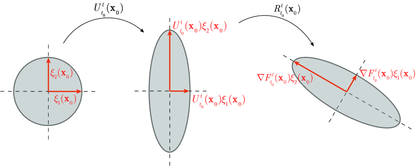
Figure 1: The action of the deformation gradient $\boldsymbol{\nabla}\mathbf{F}_{t_{0}}^{t}$ is uniquely decomposable into positive definite stretch by $\mathbf{U}_{t_{0}}^{t}$ followed by rotation by $\mathbf{R}_{t_{0}}^{t}$. This results in the polar decomposition $\boldsymbol{\nabla}\mathbf{F}_{t_{0}}^{t}=\mathbf{R}_{t_{0}}^{t}\mathbf{U}_{t_{0}}^{t}$.

When mapped forward under the deformation gradient $\nabla\mathbf{F}_{t_{0}}^{t}$, a general unit vector $\mathbf{a}$ experiences two stages of rotation. First, $\mathbf{a}$ is rotated (and simultaneously stretched) by the stretch tensor $\mathbf{U}_{t_{0}}^{t}$ into the vector $\mathbf{U}_{t_{0}}^{t}\mathbf{a}$. This first stage of rotation is entirely due to shear, with the magnitude and axis of rotation depending on $\mathbf{a}$. The second stage of rotation experienced by $\mathbf{a}$ is due to the rotation tensor $\mathbf{R}_{t_{0}}^{t}$, which rotates $\mathbf{a}$ into its final position $\mathbf{R}_{t_{0}}^{t}\mathbf{U}_{t_{0}}^{t}\mathbf{a}$ at time $t$. This second rotation acts in the same way on all $\mathbf{U}_{t_{0}}^{t}\mathbf{a}$ vectors by the proper orthogonal nature of $\mathbf{R}_{t_{0}}^{t}$.

Formed by the eigenvectors of $\mathbf{C}_{t_{0}}^{t}$, the principle rectangle illustrated in Fig. 2 has a special feature: it is the unique rectangle on which the first stage of rotation under $\mathbf{U}_{t_{0}}^{t}$ is inactive. This is because the edges of the principal rectangle align with the eigenvectors of $\mathbf{U}_{t_{0}}^{t}$ (cf. eq. (8) and Fig. 1), and hence remain unrotated by $\mathbf{U}_{t_{0}}^{t}$. The total rotation experienced by the edges of the principal rectangle is, therefore, just the rigid-body rotation exerted by the rotation tensor $\mathbf{R}_{t_{0}}^{t}$.

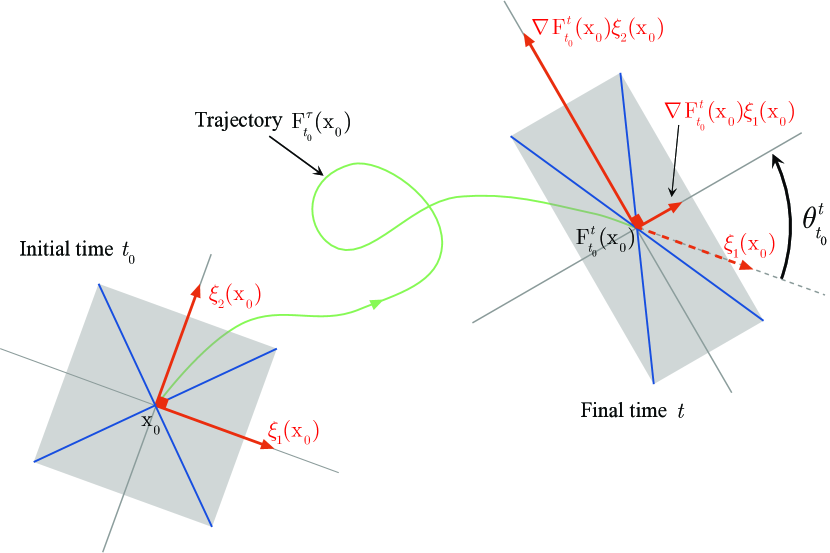
Figure 2: Finite-time deformation of an area element of a two-dimensional phase space under the flow map $\mathbf{F}_{t_{0}}^{t}$. The orthonormal basis $\{\boldsymbol{\xi}_{1},\boldsymbol{\xi}_{2}\}$ is mapped to the orthogonal basis $\{\boldsymbol{\nabla}\mathbf{F}_{t_{0}}^{t}\boldsymbol{\xi}_{1},\boldsymbol{\nabla}\mathbf{F}_{t_{0}}^{t}\boldsymbol{\xi}_{2}\}$. Other initially orthogonal material elements, such as the diagonals shown in blue, are mapped to non-orthogonal material elements.

Formula (9) shows the difference between instantaneous Eulerian rotation measured by the vorticity tensor $\mathbf{W}$ and finite-time material rotation measured by $\mathbf{R}_{t_{0}}^{t}$. In particular, at an initial time $t_{0}$, we have

$$\dot{\mathbf{R}}_{t_{0}}^{t}\big{|}_{t={t_{0}}}=\mathbf{W}(\mathbf{x}_{0},t_{0}),$$

but $\dot{\mathbf{R}}_{t_{0}}^{t}$ differs from the vorticity tensor $\mathbf{W}(\mathbf{x}(t),t)$ for times $t\neq t_{0}$.

3 Polar rotation angle (PRA)

The classic procedure for computing the polar decomposition in continuum mechanics starts with determining $\mathbf{U}_{t_{0}}^{t}$as the principal square root of the Cauchy–Green strain tensor (cf. formula (7)). This is the simplest to do by diagonalizing $\mathbf{C}_{t_{0}}^{t}$, taking the positive square root of its diagonal elements, and transforming back the resulting matrix from the strain eigenbasis to the original basis. Next, one obtains the rotation tensor directly from (6) as $\mathbf{R}_{t_{0}}^{t}=\nabla\mathbf{F}_{t_{0}}^{t}\left[\mathbf{U}_{t_{0}}^{t}\right]^{-1}$. More efficient numerical procedures are also available (see [31] and the references cited therein)

These computational approaches, however, offer little insight into the geometry of the rotation generated by $\mathbf{R}_{t_{0}}^{t}$. Taking a more geometric approach, one may recall that any three-dimensional rotation $\mathbf{R}_{t_{0}}^{t}$ has a Rodrigues representation [32] of the form

$$\mathbf{R}_{t_{0}}^{t}=\mathbf{I}+\sin\theta_{t_{0}}^{t}\mathbf{P}_{t_{0}}^{t}+(1-\cos\theta_{t_{0}}^{t})\left[\mathbf{P}_{t_{0}}^{t}\right]^{2},$$ (10)

where $\mathbf{I}$ is the $3\times 3$ identity matrix and $\mathbf{P}_{t_{0}}^{t}$ is a $3\times 3$ skew-symmetric matrix such that

$$\mathbf{P}_{t_{0}}^{t}\mathbf{a}=\mathbf{r}_{t_{0}}^{t}\times\mathbf{a},\quad\forall\mathbf{a}\in\mathbb{R}^{3}.$$

The unit vector $\mathbf{r}_{t_{0}}^{t}$ is the eigenvector of $\mathbf{R}_{t_{0}}^{t}$ corresponding to its unit eigenvalue, i.e.,

$$\mathbf{R}_{t_{0}}^{t}(\mathbf{x}_{0})\mathbf{r}_{t_{0}}^{t}(\mathbf{x}_{0})=\mathbf{r}_{t_{0}}^{t}(\mathbf{x}_{0}).$$ (11)

For planar flows, the eigenvector $\mathbf{r}_{t_{0}}^{t}$ is the unit normal to the plane of motion, and hence is independent of $\mathbf{x}_{0}$. In three-dimensions, $\mathbf{r}^{t}_{t_{0}}$ depends on the location $\mathbf{x}_{0}$ in a way discussed in the next section (cf. Proposition 1)

Once an orientation for the unit vector $\mathbf{r}_{t_{0}}^{t}(\mathbf{x}_{0})$ is selected, the angle $\theta_{t_{0}}^{t}(\mathbf{x}_{0})\in[0,2\pi)$ is uniquely determined. This angle measures the amount of local solid–body rotation experienced by material elements along the trajectory $\mathbf{x}(t;t_{0},\mathbf{x}_{0})$.

Definition 1.

We refer to the scalar function

$$\theta_{t_{0}}^{t}(\mathbf{x}_{0})\in[0,2\pi)$$

determined by (10) as the polar rotation angle (PRA) at the initial condition $\mathbf{x}_{0}$ with respect to the time interval $[t_{0},t]$.

4 Computing the PRA

Taking the trace of both sides in (10), then taking the skew-symmetric part of both sides of (10) yields the formulas

$$\cos\theta_{t_{0}}^{t} =\frac{1}{2}\left(\mathrm{tr}\,\mathbf{R}_{t_{0}}^{t}-1\right),$$ (12a)

$$\sin\theta_{t_{0}}^{t} =\frac{\left[\hat{\mathbf{R}}_{t_{0}}^{t}\right]_{ij}}{\left[\mathbf{P}_{t_{0}}^{t}\right]_{ij}}\quad(i\neq j),\qquad\hat{\mathbf{R}}_{t_{0}}^{t}:=\frac{1}{2}\left(\mathbf{R}_{t_{0}}^{t}-\left[\mathbf{R}_{t_{0}}^{t}\right]^{T}\right).$$ (12b)

To evaluate the expression for $\cos\theta_{t_{0}}^{t}$ in (12a), Guan-Suo [33] expressed $\mathrm{tr}\,\mathbf{R}_{t_{0}}^{t}$ as a somewhat cryptic function of the scalar invariants of the matrices $\nabla\mathbf{F}_{t_{0}}^{t}$, $\frac{1}{2}\left(\nabla\mathbf{F}_{t_{0}}^{t}+\left[\nabla\mathbf{F}_{t_{0}}^{t}\right]{}^{\top}\right)$ and $\mathbf{U}_{t_{0}}^{t}$. Here we derive a simply computable and intuitive alternative that only involves quantities arising in typical Lagrangian coherent structure calculations [15]: the deformation gradient, and the eigenvalues and eigenvectors of the the Cauchy–Green strain tensor.

Proposition 1.

1. In three-dimensional flows, the PRA satisfies the relations

   $$\cos\theta_{t_{0}}^{t} =\frac{1}{2}\left(\sum_{i=1}^{3}\frac{\left\langle\boldsymbol{\xi}_{i},\nabla\mathbf{F}_{t_{0}}^{t}\boldsymbol{\xi}_{i}\right\rangle}{\sqrt{\lambda_{i}}}-1\right),$$ (13a)

   $$\sin\theta_{t_{0}}^{t} =\frac{\left\langle\boldsymbol{\xi}_{i},\nabla\mathbf{F}_{t_{0}}^{t}\boldsymbol{\xi}_{j}\right\rangle-\left\langle\boldsymbol{\xi}_{j},\nabla\mathbf{F}_{t_{0}}^{t}\boldsymbol{\xi}_{i}\right\rangle}{2\epsilon_{ijk}e_{k}},\qquad i\neq j\in\{1,2,3\},$$ (13b)

   where $\mathbf{e}=(e_{1},e_{2},e_{3})^{\top}$ is the normalized eigenvector corresponding to the unit eigenvalue of the matrix

   $$\left[\mathbf{K}_{t_{0}}^{t}\right]_{jk}=\frac{\left\langle\boldsymbol{\xi}_{j},\nabla\mathbf{F}_{t_{0}}^{t}\boldsymbol{\xi}_{k}\right\rangle}{\sqrt{\lambda_{k}}},\quad j,k\in\{1,2,3\},$$

   and $\epsilon_{ijk}$ is the Levi-Civita symbol. Furthermore, we have $\mathbf{e}=\mathbf{r}_{t_{0}}^{t}$ where $\mathbf{r}_{t_{0}}^{t}$ is the axis of rotation defined by (11).

2. In two-dimensional flows, we have

   $$\cos\theta_{t_{0}}^{t} =\frac{\left\langle\boldsymbol{\xi}_{i},\nabla\mathbf{F}_{t_{0}}^{t}\boldsymbol{\xi}_{i}\right\rangle}{\sqrt{\lambda_{i}}},\qquad i=1\;\mbox{or}\;\,2,$$ (14a)

   $$\sin\theta_{t_{0}}^{t} =\left(-1\right)^{j}\frac{\left\langle\boldsymbol{\xi}_{i},\nabla\mathbf{F}_{t_{0}}^{t}\boldsymbol{\xi}_{j}\right\rangle}{\sqrt{\lambda_{j}}},\qquad\left(i,j\right)=\left(1,2\right)\quad\mbox{or}\quad\left(2,1\right),$$ (14b)

   where $\lambda_{1}\leq\lambda_{2}$ are the eigenvalues of the two-dimensional Cauchy–Green strain tensor with corresponding eigenvectors $\boldsymbol{\xi}_{1}$ and $\boldsymbol{\xi}_{2}$.

Proof.

See Appendix A. ∎

Using both expressions in the formulas (13) (or formulas (14), in the two-dimensional case), the four-quadrant polar rotation angle $\theta_{t_{0}}^{t}\in[0,2\pi)$ can be reconstructed as

$$\theta_{t_{0}}^{t}=\left[1-{\rm sign\,}\left(\sin\theta_{t_{0}}^{t}\right)\right]\pi+{\rm sign\,}\left(\sin\theta_{t_{0}}^{t}\right)\cos^{-1}\left(\cos\theta_{t_{0}}^{t}\right),$$ (15)

where

$$\rm{sign}(\alpha)=\left\{\begin{array}[]{l l}1&\qquad\rm{if}\quad\alpha\geq 0\\ -1&\qquad\rm{if}\quad\alpha<0\end{array}\right.$$

For completeness, in Appendix B, we also derive a formula for the total rotation of an arbitrary material element, not just for the strain eigenvectors. Evaluating this general formula is computationally more costly, as it involves advecting initial directions by the flow map through all intermediate times within the interval $[t_{0},t]$. In addition, due to the non-rigid-body nature of deformation along a trajectory, the total material rotation will be different for different material elements. When evaluated on initial directions aligned with $\boldsymbol{\xi}_{1}$ and $\boldsymbol{\xi}_{2}$, however, this total Lagrangian rotation agrees with the PRA modulo multiples of $2\pi$.

5 Polar LCS

A recent approach to the systematic detection of elliptic Lagrangian coherent structures (LCS) targets closed material lines that exhibit no filamentation over the finite time interval $[t_{0},t]$ (Haller and Beron-Vera [13], Haller [15]). These elliptic LCSs turn out to be uniformly stretching closed material lines, i.e., all their subsets exhibit the same relative stretching. Outermost members of nested elliptic LCS families then serve as the ideal boundaries of perfectly coherent elliptic islands.

Here we propose a dual approach to elliptic LCSs by requiring uniformity in the polar rotation of material elements forming the LCS, as opposed to uniformity in their stretching.

Definition 2.

A polar Lagrangian coherent structure (polar LCS) over the time interval $[t_{0},t]$ is a closed (i.e., tubular in 3D and circular in 2D) and connected codimension-one material surface whose time $t_{0}$ position is a level set of $\theta_{t_{0}}^{t}(\mathbf{x}_{0})$.

As any material surface, a polar LCS is invariant under the flow. It is formed by trajectories starting from a closed and connected level set of $\theta_{t_{0}}^{t}(\mathbf{x}_{0})$ at time $t_{0}$. The following simple observation shows that polar LCSs can be detected as connected and closed level sets of trigonometric functions of $\theta_{t_{0}}^{t}(\mathbf{x}_{0})$, and hence are directly computable from the formulas (13)-(14).

Proposition 2.

Connected components of the level sets of $\cos\theta_{t_{0}}^{t}$ and $\sin\theta_{t_{0}}^{t}$coincide with connected components of the level sets of $\theta_{t_{0}}^{t}(\mathbf{x}_{0})$.

Proof.

Assume the contrary, i.e., the existence of two points $\mathbf{x}_{0}$ and $\mathbf{\hat{x}}_{0}$ that are in the same connected component of a level set $\mathcal{L}$ of $\cos\theta_{t_{0}}^{t}(\mathbf{x}_{0})$ but on different connected level sets of $\theta_{t_{0}}^{t}(\mathbf{x}_{0})$. Then on any continuous path connecting $\mathbf{x}_{0}$ and $\mathbf{\hat{x}}_{0}$, the polar rotation angle $\theta_{t_{0}}^{t}$ should change continuously from $\theta_{t_{0}}^{t}(\mathbf{x}_{0})$ to $\theta_{t_{0}}^{t}(\mathbf{\hat{x}}_{0})\neq\theta_{t_{0}}^{t}(\mathbf{x}_{0}),$ and hence $\cos\theta_{t_{0}}^{t}$ cannot be constant along this path. Since $\mathbf{x}_{0}$ and $\mathbf{\hat{x}}_{0}$ are in the connected set $\mathcal{L}$, there is therefore a continuous path connecting $\mathbf{x}_{0}$ and $\mathbf{\hat{x}}_{0}$ within $\mathcal{L}$ along which $\cos\theta_{t_{0}}^{t}(\mathbf{x}_{0})$ cannot be constant. But this contradicts the assumption that $\mathcal{L}$ is a level set of $\cos\theta_{t_{0}}^{t}(\mathbf{x}_{0})$. The argument for $\sin\theta_{t_{0}}^{t}$ is identical. ∎

A practical consequence of Proposition 2 is that connected level sets of $\theta_{t_{0}}^{t}(\mathbf{x}_{0})$ can be constructed as those of $\cos\theta_{t_{0}}^{t}$ and $\sin\theta_{t_{0}}^{t}$, without verifying the orientability of $\mathbf{r}_{t_{0}}^{t}(\mathbf{x}_{0})$ on $U$. This renders the computation of the tensor $\mathbf{K}_{t_{0}}^{t}$ and the rotation axis $\mathbf{r}_{t_{0}}^{t}$ unnecessary, as one can compute the two-quadrant angle $\theta_{t_{0}}^{t}\in[0,\pi]$ from equation (13a) as

$$\theta_{t_{0}}^{t}=\cos^{-1}\left[\frac{1}{2}\left(\sum_{i=1}^{3}\frac{\left\langle\boldsymbol{\xi}_{i},\nabla\mathbf{F}_{t_{0}}^{t}\boldsymbol{\xi}_{i}\right\rangle}{\sqrt{\lambda_{i}}}-1\right)\right].$$ (16)

Proposition 2 ensures that the level sets of $\theta^{t}_{t_{0}}$ computed from (16) coincide with those of the four-quadrant PRA angle computed from (15).

All quantities derived from the deformation gradient $\boldsymbol{\nabla}\mathbf{F}_{t_{0}}^{t}$ are invariant with respect to time-dependent translations of the coordinate frame. Therefore, polar LCSs are Galilean invariant objects. For two-dimensional flows, polar LCSs also turn out to be invariant under time-dependent rotations of the frame. In the language of continuum mechanics [29], polar LCSs in two dimensions are objective.

Proposition 3.

In two-dimensional flows, a polar LCS over the time interval $[t_{0},t]$ is objective, i.e., invariant under coordinate changes of the form

$$\mathbf{x}=\mathbf{Q}(t)\mathbf{y}+\mathbf{b}(t),$$ (17)

where $\mathbf{Q}(t)\in SO(2)$ and $\mathbf{b}(t)\in\mathbb{R}^{2}$ are smooth functions of time $t$.

Proof.

See Appendix C. ∎

An elliptic island marked by the PRA has a natural center point: the PRA extremum point surrounded by closed PRA contours. This leads to the following definition of a Lagrangian vortex center:

Definition 3.

A Lagrangian vortex center over the time interval $[t_{0},t]$ is a set of trajectories evolving from a connected, codimension-two level set of $\theta_{t_{0}}^{t}(\mathbf{x}_{0})$.

A Lagrangian vortex center identified from the PRA is, therefore, composed of a single trajectory in two dimensions and of a one-parameter family of trajectories (i.e., a material line) in three dimensions. Despite recent progress in the accurate detection of coherent Lagrangian vortex boundaries [15], approaches to Lagrangian vortex center definition and detection have notably been missing. As we illustrate in Section 6.2 below, vortex centers defined as PRA extrema indeed show distinguished behavior: they capture the translational motion of an elliptic island without being affected by the rotational motion of trajectories inside the island. As connected level sets of the PRA, the Lagrangian vortex centers defined in Definition 3 are also objective in two-dimensional flows (cf. Proposition 17).

6 Examples

In this section, we compute the PRA on several examples to illustrate how its closed level curves (i.e., initial positions of polar LCSs) highlight the internal structure of elliptic islands in detail.

6.1 Standard map

We first consider the standard map

$$I_{n+1} =I_{n}+\epsilon\sin\phi_{n},$$

$$\phi_{n+1} =\phi_{n}+I_{n+1},$$ (18)

which is a Poincaré map $\mathcal{P}$ of a rotor excited by a periodic impulsive force [34]. In the absence of the impulse, i.e., for $\epsilon=0$, the angular momentum $I_{n}$ is constant and the angular position $\phi_{n}$ increases linearly as an integer multiple of the angular momentum.

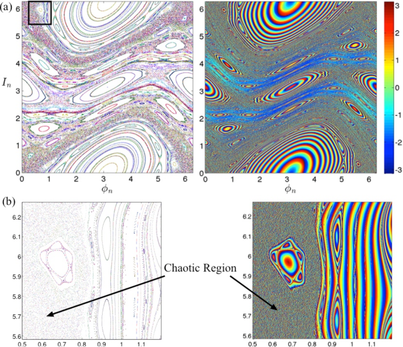
Figure 3: Standard map. (a) Left: $1000$ iterations of the standard map for $400$ uniformly distributed initial conditions over the torus $[0,2\pi]\times[0,2\pi]$. Right: The PRA $\theta_{t_{0}}^{t}$ for $200$ iterations of the standard map, clearly marking polar LCSs (closed contours) and Lagrangian vortex centers (local extrema) (b) The close-up view of the region marked by a rectangle in (a).

For $\epsilon\neq 0$, however, the system can exhibit complicated dynamics. Depending on the initial condition $(I_{0},\phi_{0})$, the trajectories may be periodic, quasi-periodic or chaotic. The quasi-periodic trajectories lie on KAM tori, the classic examples of vortical structures that we wish to visualize through the PRA.

The left plot in Fig. 3a shows $1000$ iterations of the standard map for $400$ uniformly distributed initial conditions and $\epsilon=1$. This reveals invariant KAM tori, resonance islands and chaotic regions. The right panel of the same figure shows the PRA, computed from formula (15) with $i=2$, with the flow map being equal to $200$ iterations of the map (18), i.e. $\mathbf{F}_{t_{0}}^{t}(\mathbf{x}_{0})=\mathcal{P}^{200}(\mathbf{x}_{0})$, where $\mathbf{x}_{0}=(\phi_{0},I_{0})$ and $(\phi_{n+1},I_{n+1})=\mathcal{P}(\phi_{n},I_{n})$. To ensure the accuracy of the finite differences for the computation of the deformation gradient $\boldsymbol{\nabla}\mathbf{F}_{t_{0}}^{t}$, we use a dense grid of initial conditions consisting of $1000\times 1000$ uniformly distributed points over the phase space $\mathbb{T}^{2}=[0,2\pi]\times[0,2\pi]$.

Figure 3b shows a close-up of a region of the phase space containing chaotic trajectories, KAM tori and a period-$5$ resonance island. For this close-up view, the Poincaré map is recomputed from $1000$ iterations of $2500$ initial conditions. The corresponding PRA plot on the right is computed only from $500$ iterations, i.e., from $\mathbf{F}_{t_{0}}^{t}=\mathcal{P}^{500}$.

We conclude that the KAM tori and resonance islands are sharply enhanced by the PRA relative to a simple iteration of the map, even though the number of iterations used in constructing the PRA plot is only half the number used for the Poincaré map. The chaotic region is marked by small-scale rapid variations in the PRA, in line with the sensitive dependence of the rotation angle on initial conditions in these regions.

Figure 3 also shows that the center-type fixed points in the elliptic islands are clearly marked with local extrema of the PRA, supporting the idea of defining Lagrangian elliptic centers as stated in Definition 3.

6.2 Two-dimensional turbulence

Consider the Navier–Stokes equation

$$\partial_{t}\mathbf{u}+\mathbf{u}\cdot\mathbf{\boldsymbol{\nabla}}\mathbf{u}=-\boldsymbol{\nabla}p+\nu\Delta\mathbf{u}+\mathbf{f},\ \ \ \boldsymbol{\nabla}\cdot\mathbf{u}=0,$$ (19)

where $\nu$ is the kinematic viscosity and $\mathbf{f}$ denotes the forcing. For an ideal two-dimensional fluid flow ($\nu=0$ and $\mathbf{f}=\mathbf{0}$ ), the vorticity $\omega$, given by $\boldsymbol{\nabla}\times\mathbf{u}=(0,0,\omega)$, is preserved along fluid trajectories, i.e.,

$$\frac{\mathrm{D}\omega}{\mathrm{D}t}=0,$$ (20)

where $\frac{\mathrm{D}\;}{\mathrm{D}t}:=\partial_{t}+\mathbf{u}\cdot\boldsymbol{\nabla}$ is the material derivative. Therefore, closed level curves of vorticity are material curves, acting as barriers to the transport of fluid particles. In the presence of molecular diffusion and external forcing, however, vorticity is not a material invariant and hence its closed contours no longer signal elliptic islands for fluid trajectories.

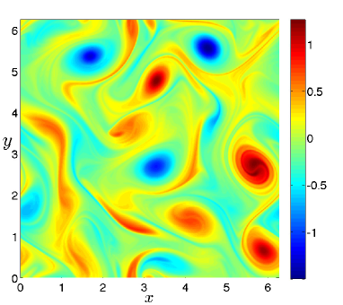
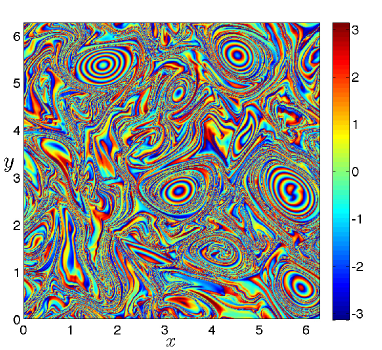
Figure 4: Left: Vorticity $\omega$ at the initial time $t=50$. Right: The PRA $\theta_{t_{0}}^{t}$ computed from formula (15) over the time interval $[50,100]$.

To illustrate the use of PRA in detecting elliptic islands in a turbulent flow, we solve the Navier–Stokes equation (19) with $\nu=10^{-5}$ on the domain $\mathcal{D}=[0,2\pi]\times[0,2\pi]$ with periodic boundary conditions. We use a pseudo-spectral method with $512^{2}$ modes to evaluate the spatial partial derivatives and the nonlinear term. The external forcing is random in phase and only active over the wave-numbers $3.5<k<4.5$. The forcing amplitude is time-dependent and chosen to balance the instantaneous enstrophy dissipation $-\nu\int_{U}|\boldsymbol{\nabla}\omega(\mathbf{x},t)|^{2}\mbox{d}\mathbf{x}$. The time integration is carried out by a variable step-size, fourth-order Runge–Kutta method [35]. We solve the equation up to time $t=100$. We observe that the turbulent flow is fully developed after $50$ time units. Therefore, we choose times $t_{0}=50$ and $t=100$ as the initial and final times for the computation of the PRA $\theta_{t_{0}}^{t}$.

Such two-dimensional turbulent flows tend to generate long-lasting coherent vortices [36], which are also prevalent in geophysical flows [37]. Highly coherent Lagrangian signatures of such vortices have been recently identified as regions bounded by uniformly stretching material lines [13, 15].

Here, we take an alternative approach and identify coherent Lagrangian vortices as regions filled with polar LCSs. In other words, we seek the elliptic islands of turbulence as regions of closed material lines that pointwise have the same rigid-body rotation component in their deformation over the time interval of interest.

Figure 4 (right panel) shows the PRA computed from formula (15) for $512\times 512$ uniformly distributed initial conditions. The polar LCSs are clearly visible as concentric closed contours of $\theta_{t_{0}}^{t}(\mathbf{x}_{0})$. Figure 5 shows a closeup view of a coherent Lagrangian vortex identified from the PRA plot. Note how the PRA shows a sharp distinction between the vortical region and the surrounding chaotic background. As in the case of the standard map (see Fig. 3), the chaotic region is marked by small-scale, sharp variations of the Lagrangian rotation due to sensitive dependence of material rotation angle on initial conditions.

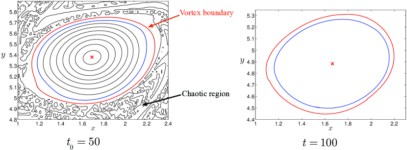
Figure 5: Left: Contours of the PRA signaling coherent and chaotic regions. Right: Advected image of select contours to the final time $t=100$. The local extremum of the PRA (marked by a cross) defining the Lagragian vortex center by Definition 3.

While the velocity field is well-resolved, resolving small-scale Lagrangian structures requires significantly higher resolution [38, 39, 40]. At the present resolution, the Lagrangian structures in the chaotic region are not well-resolved. Nonetheless, the boundary of the vortex can be approximated by the contour across which the PRA transitions from concentric large-scale contours to small-scale sharp variations (see the red-colored contour in Fig. 5).

We now illustrate that the large-scale polar LCSs, defined by closed contours of the PRA (cf. Definition 2) indeed remain coherent under advection. We advect two such contours under the flow, with their advected positions shown in the right panel on Fig. 5 at time $t=100$.

As a measure of coherence we define relative stretching of material lines as $\left[\ell(t)-\ell(t_{0})\right]/\ell(t_{0})$, where $\ell$ denotes the length of the material line as a function of time. The relative stretching of the blue and red contours are $2.65\%$ and $-1.38\%$, respectively. These relative stretching values remain in the order of stretching exhibited by perfectly coherent elliptic LCSs obtained from the geodesic LCS theory [13].

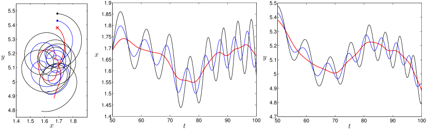
Figure 6: Left panel: Trajectories of the Lagrangian vortex center (red) and nearby passive tracers (blue and black). Middle and Right panels: The coordinates of the vortex center and nearby tracers as a function of time.

The cross in Fig. 5 marks a local extremum of the PRA, which is a Lagrangian vortex center by our Definition 3. This local extremum indeed turns out to behave as the vortex center over the time interval of interest, i.e., $t\in[50,100]$. Figure 6 shows the trajectory starting from this PRA extremum, whose initial coordinates are $(1.690,5.380)$. For reference, two other trajectories are also shown with initial positions at $0.05$ and $0.1$ distance from the vortex center. Due to the complexity of the flow, the trajectory patterns are not illuminating. However, their $x$- and $y$-coordinates as a function of time reveal the oscillatory motion of nearby trajectories around the vortex center, while the vortex center itself has minimal oscillations (cf. middle and right panels of Fig. 6). The oscillations of the vortex center are due to the motion of the vortex as a whole. The nearby trajectories, however, exhibit higher frequency oscillations which are due to their swirling motion around the vortex center.

6.3 Stratified geophysical fluid flow

We consider a simplified model for stratified geophysical fluid flow, the barotropic equation. This equation, in the vorticity-stream form, reads [41]

$$\partial_{t}\omega+J(\psi,\omega)+\partial_{x}\psi=0,\ \ \ \omega=\Delta\psi,$$ (21)

where $w(x,y,t)$ and $\psi(x,y,t)$ are non-dimensional vorticity and stream function, respectively. In deriving this equation, the viscous dissipation is neglected and the Coriolis frequency is assumed to be linear in the meridional coordinate $y$ (i.e., the $\beta$-plane approximation is used [41]). The Jacobian operator reads $J(\psi,\omega)=\partial_{x}\psi\partial_{y}\omega-\partial_{y}\psi\partial_{x}\omega$. The fluid velocity field $\mathbf{u}$ is given in terms of the stream function by $\mathbf{u}=(\partial_{y}\psi,-\partial_{x}\psi)$.

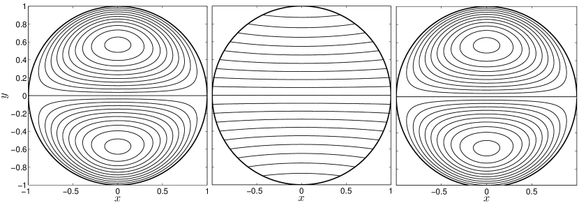
Figure 7: Contours of the stream function $\psi$ (left), vorticity $\omega$ (middle) and potential vorticity $q$ (right) of the modon solution (22).

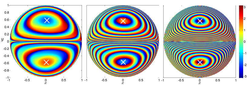
Figure 8: The PRA for the modon solution (22). The initial time is $t_{0}=0$ and the final times are $t=100$ (left), $t=250$ (middle) and $t=500$ (right). All figures are computed from a grid of roughly $35$ thousand uniformly distributed initial conditions in the unit disk. The points marked by crosses are the Lagrangian vortex centers obtained from Definition 3 over the corresponding time intervals.

Vorticity is not preserved along fluid trajectories when the flow satisfies (21). Instead, one can show that the potential vorticity $q=\omega+y$ is conserved along these trajectories (see, e.g., [41]).

We consider a steady exact solution of the barotropic equation (21) called a modon: a uniformly propagating vortex dipole. For this modon solution, the stream function and vorticity are given respectively by

$$\psi(r,\varphi)=\left(\frac{J_{1}(r)}{J_{1}(1)}-r\right)\sin\varphi, 0\leq r\leq 1$$

$$\omega(r,\varphi)=-\frac{J_{1}(r)}{J_{1}(1)}\sin\varphi, 0\leq r\leq 1$$ (22)

in polar coordinates $(r,\varphi)$ where $r=\sqrt{x^{2}+y^{2}}$, $\tan\varphi=y/x$ and $J_{1}$ is the Bessel function of the first kind [42]. This solution is written in a frame co-moving with the modon at a constant speed $c=1$.

The stream function $\psi$ defines a flow on the invariant domain $r\leq 1$. While this solution can, in principle, be extended to the entire plane [42, 43], here we only consider the motion inside the unit disk.

Figure 7 shows the stream function, the vorticity and the potential vorticity for the modon solution (22). Since the flow is integrable, its stream function completely describes the flow structure, showing two counter-rotating vortices.

The vorticity $\omega$ is negative in the upper half-disk $y>0$ and positive in the lower half-disk $y<0$. Its contours, however, do not reveal the two vortices present in the flow. This is because unlike the two-dimensional Euler flows, vorticity is not conserved along the trajectories of the solutions of the barotropic equation (21).

The potential vorticity $q$, as a conserved quantity, reveals the eddies. Its level curves (Fig. 7, right panel) resemble those of the streamlines. In fact, the particular solution (22) of the barotropic equation satisfies $q=-\psi$.

Figure 8 shows the PRA for integration times $t=100$, $250$ and $500$. The integration time $t=100$ is chosen such that almost all periodic orbits of $\dot{\mathbf{x}}=\mathbf{u}(\mathbf{x})$ complete at least one period. Even with this relatively short integration time, PRA contours already reveal the vortices. Obtained from a finite-time assessment of the flow, the PRA contours deviate from the trajectories. As the integration time increases, however, the PRA contours converge to the streamlines and Lagrangian vortex centers obtained from the PRA converge to the elliptic fixed points of the flow.

6.4 ABC flow

As our last example, we consider the Arnold-Beltrami–Childress (ABC) flow $\dot{\mathbf{x}}=\mathbf{u}(\mathbf{x})$ where

$$\mathbf{u}(\mathbf{x})=\begin{pmatrix}A\sin(z)+C\cos(y)\\ B\sin(x)+A\cos(z)\\ C\sin(y)+B\cos(x)\end{pmatrix},$$ (23)

with $\mathbf{x}=(x,y,z)$ and $A,B,C\in\mathbb{R}$ are constant parameters [2]. The velocity field $\mathbf{u}$ is an exact steady solution of Euler’s equation for inviscid Newtonian fluids with periodic boundary conditions. The ABC velocity field is a Beltrami vector field satisfying $\boldsymbol{\omega}(\mathbf{x})=\mathbf{u}(\mathbf{x})$ with $\boldsymbol{\omega}=\boldsymbol{\nabla}\times\mathbf{u}$ being the vorticity field.

In the following, we set $A=1$, $B=\sqrt{2/3}$ and $C=\sqrt{1/3}$. The Lagrangian computations are carried out on a uniform grid of $200\times 200\times 200$ initial conditions distributed over the domain $\mathbb{T}^{3}\in[0,2\pi]\times[0,2\pi]\times[0,2\pi]$.

Figure 9 (left panel) shows the helicity density $\langle\mathbf{u},\boldsymbol{\omega}\rangle$ (=$|\boldsymbol{\omega}|^{2}$). While such Eulerian features may suggest coherent vortical motion throughout the domain, the ABC flow is known to have chaotic fluid trajectories in addition to coherent swirling trajectories lying on invariant tori [44].

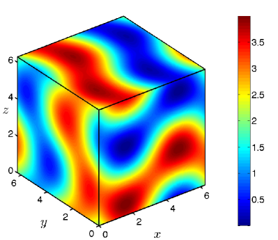
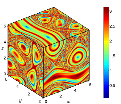
Figure 9: Left: The helicity $\langle\mathbf{u},\boldsymbol{\omega}\rangle=|\boldsymbol{\omega}|^{2}$ for the ABC flow. Right: The two-quadrant PRA $\theta_{t_{0}}^{t}$ with the integration time $t-t_{0}=50$, computed from formula (16).

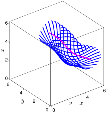
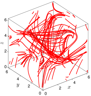
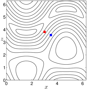
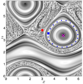
Figure 10: Top: Two trajectories of the ABC flow. The blue trajectory starts in an elliptic island and traces the surface of an invariant torus. The red trajectory is chaotic. Note that the trajectories are plotted modulo $2\pi$. The material line marking the Lagrangian vortex core (cf. Definition 3) is plotted in magenta color. Bottom: The initial condition (squares) of each trajectory is superimposed on the $y=0$ slice of the helicity $\langle\mathbf{u},\boldsymbol{\omega}\rangle=|\boldsymbol{\omega}|^{2}$ (left) and the PRA $\theta_{t_{0}}^{t}$ obtained from formula (16) (right). The right panel also shows the intersections of the blue trajectory with the plane $y=0$ (blue dots), as well as the vortex core (magenta cross).

These invariant tori form vortical regions that we seek to capture from finite-time flow samples as elliptic regions. Using a local variational principle extremizing Lagrangian shear, elliptic LCSs approximating the tori from finite-time flow samples have been constructed by Blazevski and Haller [14]. Here we illustrate that polar LCSs obtained from the PRA also give a close approximation at a reduced computational cost.

Indeed, the PRA admits tubular level surfaces that closely approximate the invariant tori (Fig. 9, right panel). Codimension-two level sets of the PRA are periodic material curves at the cores of the elliptic regions. These material lines serve as Lagrangian vortex centers by Definition 3. As in earlier examples, outside the elliptic islands formed by these closed level surfaces, PRA levels exhibit small-scale variations due to sensitive dependence of the rotation angle on the initial conditions.

To examine how accurately the PRA field $\theta_{t_{0}}^{t}$ captures the tori and the chaotic region boundaries, we release two trajectories from the initial conditions $\mathbf{x}_{0}=(3.085,0,3.820)$ (red square in the bottom panel of Fig. 10) and $\mathbf{x}_{0}=(3.505,0,3.568)$ (blue square in the bottom panel of Fig. 10). The initial conditions are chosen such that they are nearby, yet one belongs to the chaotic region (red square) and the other (blue square) belongs to a smooth level-surface of the PRA signaling an invariant torus.

These initial conditions are then advected under the ABC flow from time $t=0$ to $t=500$. The resulting trajectories are shown in the top panel of Fig. 10. As expected, the blue trajectory remains on a torus while the red trajectory exhibits chaotic behavior. Note that all curves correspond to a single trajectory and only appear as line segments because they are plotted modulo $2\pi$. The intersections of the coherent trajectory with the Poincaré section $y=0$ shows that the PRA captures the invariant torus accurately (Fig. 10, bottom panel).

We stress that both initial conditions studied here belong to topologically equivalent regions of the local helicity $\langle\mathbf{u},\boldsymbol{\omega}\rangle=|\boldsymbol{\omega}|^{2}$. The vorticity magnitude, therefore, fails to distinguish vortical regions from chaotic regions. This is because vorticity magnitude is not a material invariant of the Euler’s equation in three dimensions and therefore does not generally capture material behavior.

7 Conclusions

Most approaches to coherent structures seek their signature in material separation or stretching. By contrast, we have developed here an approach to locate coherent structures based on their signature in material rotation. To quantify finite material rotation in a mathematically precise fashion, we have used the polar rotation tensor from the unique rotation-stretch factorization of the deformation gradient.

For two- and three-dimensional dynamical systems, we have derived explicit formulas for the polar rotation angle (PRA) generated by the rotation tensor around its axis of rotation. While polar rotation has broadly been studied and used in continuum mechanics, the simple formulas we have derived here for the PRA in terms of the flow gradient, its singular values and singular vectors have not been available. These formulas enable the efficient computation of the PRA from basic quantities provided by existing numerical algorithms for Lagrangian coherent structure detection.

Building on the PRA, we have also introduced the notion of polar Lagrangian coherent structures (polar LCSs). These are tubular material surfaces along which trajectories admit the same PRA value over a finite time interval of interest. We have proposed regions filled by polar LCSs as rotation-based generalizations of the classic elliptic islands filled by KAM tori in Hamiltonian systems.

As we demonstrated on a direct numerical simulation of two-dimensional turbulence, the PRA identifies Lagrangian vortex boundaries with high accuracy. While geodesic LCS theory of Haller and Beron-Vera [13] offers an exact detection of such vortex boundaries as solutions of differential equations, the present diagnostic detection of these boundaries as outermost closed PRA level curves is substantially less computational, and hence preferable for an approximate identification of these boundaries.

Outside the Lagrangian vortex boundaries, the PRA is dominated by small-scale noise due to its sensitive dependence on initial conditions. In these regions, therefore, the PRA displays no clear signature for hyperbolic LCSs governing chaotic tracer mixing. These latter types of LCSs, by contrast, are efficiently revealed by another objective diagnostic, the finite-time Lyapunov exponent (FTLE) [15]. The PRA and FTLE have a well-defined duality: the former is a scalar field characterizing the rotational factor $\mathbf{R}_{t_{0}}^{t}$, while the latter characterizes the stretch factor $\mathbf{U}_{t_{0}}^{t}$ in the polar decomposition $\boldsymbol{\nabla}\mathbf{F}_{t_{0}}^{t}=\mathbf{R}_{t_{0}}^{t}\mathbf{U}_{t_{0}}^{t}$ of the deformation gradient.

We have found that local extrema of the PRA mark initial positions of trajectories that serve as well-defined centers for elliptic islands. Oscillations in these center trajectories are minimal and arise solely due to the material translation of the underlying island. Nearby trajectories inside the elliptic island, on the other hand, oscillate rapidly due to their swirling motion around the center trajectory (cf. Fig. 6). The ability of the PRA to identify a unique vortex center should be helpful in Lagrangian versions of the Eulerian eddy censuses carried out by Dong et al. [45] and Chelton et al. [46].

The elliptic island boundaries marked by PRA do not necessarily remain unfilamented under advection. If the goal is to find perfectly coherent Lagrangian vortices (see, e.g., [47]), then the geodesic theory of Haller and Beron-Vera [13] should be applied. This theory identifies material vortex boundaries as closed null geodesics of the generalized Green-Lagrange strain tensor. The related computations require the a priori identification of phase space regions where such closed geodesics may exist [48]. Vortex regions identified from the PRA provide a quickly computable starting point for the detection of closed Green-Lagrange null geodesics. Incorporating the vortex centers obtained from the PRA in the geodesic LCS analysis is, therefore, expected to lead to a notable computational speed-up.

Finally, the polar LCSs obtained as level curves of the PRA are frame-invariant for planar flows (see Proposition 17). Such objectivity is desirable for coherent structure identification methods in order to exclude false positives and negatives specific to the coordinate system used in the analysis [15]. In three dimensions, however, the PRA does depend on the reference frame. The objective detection of higher-dimensional elliptic islands from their rotational coherence, therefore, requires further work.

Appendix A Proof of Proposition 1

Part (1): The trace of a tensor is independent of the choice of basis. If we represent the rotation tensor $\mathbf{R}_{t_{0}}^{t}$ in the orthonormal basis $\{\boldsymbol{\xi}_{k}\}_{1\leq k\leq 3}$, then its entires satisfy $\left[\mathbf{R}_{t_{0}}^{t}\right]_{ij}=\left\langle\boldsymbol{\xi}_{i},\mathbf{R}_{t_{0}}^{t}\boldsymbol{\xi}_{j}\right\rangle$. Therefore, using formula (8), we can write

$$\mathrm{tr}\,\mathbf{R}_{t_{0}}^{t} =\sum_{i=1}^{3}\left\langle\boldsymbol{\xi}_{i},\mathbf{R}_{t_{0}}^{t}\boldsymbol{\xi}_{i}\right\rangle=\sum_{i=1}^{3}\left\langle\boldsymbol{\xi}_{i},\nabla\mathbf{F}_{t_{0}}^{t}\left[\mathbf{U}_{t_{0}}^{t}\right]^{-1}\boldsymbol{\xi}_{i}\right\rangle$$

$$=\sum_{i=1}^{3}\left\langle\boldsymbol{\xi}_{i},\nabla\mathbf{F}_{t_{0}}^{t}\frac{1}{\sqrt{\lambda_{i}}}\boldsymbol{\xi}_{i}\right\rangle=\sum_{i=1}^{3}\frac{\left\langle\boldsymbol{\xi}_{i},\nabla\mathbf{F}_{t_{0}}^{t}\boldsymbol{\xi}_{i}\right\rangle}{\sqrt{\lambda_{i}}},$$ (24)

which, together with (12a), proves formula (13a).

To prove formula (13b), we first note the coordinate form of equation (12b):

$$\frac{1}{2}\left(\left[\mathbf{R}_{t_{0}}^{t}\right]_{ij}-\left[\mathbf{R}_{t_{0}}^{t}\right]_{ji}\right)=\sin\theta_{t_{0}}^{t}\epsilon_{ijk}\left[\mathbf{r}_{t_{0}}^{t}\right]_{k}.$$

Applying the same argument used in (24) in the strain eigenbasis, we obtain

$$\sin\theta_{t_{0}}^{t}=\frac{\left\langle\boldsymbol{\xi}_{i},\nabla\mathbf{F}_{t_{0}}^{t}\frac{1}{\sqrt{\lambda_{j}}}\boldsymbol{\xi}_{j}\right\rangle-\left\langle\boldsymbol{\xi}_{j},\nabla\mathbf{F}_{t_{0}}^{t}\frac{1}{\sqrt{\lambda_{i}}}\boldsymbol{\xi}_{i}\right\rangle}{2\epsilon_{ijk}\left[\mathbf{r}_{t_{0}}^{t}\right]_{k}},\quad i\neq j.$$ (25)

Next we write the eigenvector $\mathbf{r}_{t_{0}}^{t}$ in strain basis as $\mathbf{r}_{t_{0}}^{t}=\sum_{k}e_{k}\boldsymbol{\xi}_{k}$ to obtain

$$\sum_{k}e_{k}\boldsymbol{\xi}_{k}=\mathbf{R}_{t_{0}}^{t}\sum_{k}e_{k}\boldsymbol{\xi}_{k}=\nabla\mathbf{F}_{t_{0}}^{t}\left[\mathbf{U}_{t_{0}}^{t}\right]^{-1}\sum_{k}e_{k}\boldsymbol{\xi}_{k}=\sum_{k}\frac{e_{k}}{\sqrt{\lambda_{k}}}\nabla\mathbf{F}_{t_{0}}^{t}\boldsymbol{\xi}_{k},$$

which implies

$$e_{j}=\sum_{k}\frac{\left\langle\boldsymbol{\xi}_{j},\nabla\mathbf{F}_{t_{0}}^{t}\boldsymbol{\xi}_{k}\right\rangle}{\sqrt{\lambda_{k}}}e_{k},$$

or, equivalently, $\mathbf{K}_{t_{0}}^{t}\mathbf{e}=\mathbf{e}$, with $\mathbf{K}_{t_{0}}^{t}$ and $\mathbf{e}$ defined in the statement of Proposition 1. Since $\left[\mathbf{r}_{t_{0}}^{t}\right]_{k}=e_{k}$, formula (25) proves (13b).

Part (2): Two-dimensional flows are parallel to a distinguished plane and exhibit no stretching or shrinking along the normal of this plane. In this case, we have

$$\lambda_{1}\leq\lambda_{2}=1\leq\lambda_{3},$$

with the strain eigenvector $\boldsymbol{\xi}_{2}$ pointing in the normal of the plane in question. Formula (13) then gives

$$\cos\theta_{t_{0}}^{t}=\frac{1}{2}\left(\frac{\left\langle\boldsymbol{\xi}_{1},\nabla\mathbf{F}_{t_{0}}^{t}\boldsymbol{\xi}_{1}\right\rangle}{\sqrt{\lambda_{1}}}+\frac{\left\langle\boldsymbol{\xi}_{3},\nabla\mathbf{F}_{t_{0}}^{t}\boldsymbol{\xi}_{3}\right\rangle}{\sqrt{\lambda_{3}}}\right).$$ (26)

Restricting our consideration to the two-dimensional plane of the flow, we reindex the quantities in formula (26) as $\lambda_{3}\to\lambda_{2}$ and $\boldsymbol{\xi}_{3}\to\boldsymbol{\xi}_{2}$, given that the original $\lambda_{3}$ strain eigenvalue of the flow is the second largest principal strain in the plane of the flow. After this re-indexing, equation (26) gives

$$\cos\theta_{t_{0}}^{t}=\frac{1}{2}\sum_{i=1}^{2}\frac{\left\langle\boldsymbol{\xi}_{i},\nabla\mathbf{F}_{t_{0}}^{t}\boldsymbol{\xi}_{i}\right\rangle}{\sqrt{\lambda_{i}}}.$$ (27)

The summands in this last expression are just the diagonal elements of the two-dimensional rotation tensor $\mathbf{R}_{t_{0}}^{t}$ represented in the $\left\{\boldsymbol{\xi}_{1},\boldsymbol{\xi}_{2}\right\}$ basis (cf. our discussion leading to equation (24)). Since the diagonal elements of any two-dimensional rotation matrix are equal, formula (14a) follows from (27).

In two dimensions, the rotation tensor is of the form

$$\mathbf{R}_{t_{0}}^{t}(\mathbf{x}_{0})=\begin{pmatrix}\cos\theta_{t_{0}}^{t}(\mathbf{x}_{0})&\sin\theta_{t_{0}}^{t}(\mathbf{x}_{0})\\ -\sin\theta_{t_{0}}^{t}(\mathbf{x}_{0})&\cos\theta_{t_{0}}^{t}(\mathbf{x}_{0})\end{pmatrix}.$$ (28)

Thus, using the argument in (24), we obtain that

$$\sin\theta_{t_{0}}^{t}=\left\langle\boldsymbol{\xi}_{1},\mathbf{R}_{t_{0}}^{t}\boldsymbol{\xi}_{2}\right\rangle=\frac{\left\langle\boldsymbol{\xi}_{1},\nabla\mathbf{F}_{t_{0}}^{t}\boldsymbol{\xi}_{2}\right\rangle}{\sqrt{\lambda_{2}}}=-\left\langle\boldsymbol{\xi}_{2},\mathbf{R}_{t_{0}}^{t}\boldsymbol{\xi}_{1}\right\rangle=-\frac{\left\langle\boldsymbol{\xi}_{2},\nabla\mathbf{F}_{t_{0}}^{t}\boldsymbol{\xi}_{1}\right\rangle}{\sqrt{\lambda_{1}}},$$

whichi is the PRA formula (14b).

Appendix B Total Lagrangian rotation in planar flows

The polar rotation $\theta_{t_{0}}^{t}$ defined in Definition 1 is the net rotation of the $\{\boldsymbol{\xi}_{1},\boldsymbol{\xi}_{2}\}$ eigenbasis over the time interval $[t_{0},t].$ This quantity, however, measures the rotation modulo $2\pi$ and does not differentiate between rotation by $\theta_{0}$ and $\theta_{0}+2k\pi$. Here, we also derive an expression for the total Lagrangian rotation of the eigenbasis that distinguishes between rotations differing by an integer multiple of $2\pi$.

Consider the equations of variations for a given infinitesimal displacement $\boldsymbol{\xi}$,

$$\dot{\boldsymbol{\xi}}(t)=\boldsymbol{\nabla}\mathbf{u}(\mathbf{x}(t),t)\boldsymbol{\xi}(t).$$ (29)

Write $\boldsymbol{\xi}(t)=r\mathbf{e}_{\phi}$ where $\mathbf{e}_{\phi}=(\cos\phi,\sin\phi)^{\top}$ and $(r,\phi)$ are functions of time. Substituting this in the equations of variations (29) we get

$$\dot{r}\mathbf{e}_{\phi}+r\dot{\phi}\mathbf{e}_{\phi}^{\perp}=r\boldsymbol{\nabla}\mathbf{u}(\mathbf{x}(t),t)\mathbf{e}_{\phi},$$ (30)

with $\mathbf{e}_{\phi}^{\perp}=(-\sin\phi,\cos\phi)^{\top}$. Since $\mathbf{e}_{\phi}$ and $\mathbf{e}_{\phi}^{\perp}$ are perpendicular, we have

$$\frac{\dot{r}}{r}=\langle\mathbf{e}_{\phi},\boldsymbol{\nabla}\mathbf{u}(\mathbf{x}(t),t)\mathbf{e}_{\phi}\rangle,$$ (31a)

$$\dot{\phi}=\langle\mathbf{e}_{\phi}^{\perp},\boldsymbol{\nabla}\mathbf{u}(\mathbf{x}(t),t)\mathbf{e}_{\phi}\rangle.$$ (31b)

Therefore, solving Eq. (31b), the total rotation of an arbitrary displacement vector $\boldsymbol{\xi}_{0}=(\cos\phi_{0},\sin\phi_{0})^{\top}$ is given by

$$\theta_{\mathrm{tot}}:=\phi(t)-\phi_{0}=\int_{t_{0}}^{t}\langle\mathbf{e}_{\phi(\tau)}^{\perp},\boldsymbol{\nabla}\mathbf{u}(\mathbf{x}(\tau),\tau)\mathbf{e}_{\phi(\tau)}\rangle\mbox{d}\tau.$$ (32)

If the initial vector $\boldsymbol{\xi}_{0}$ is chosen to be $\boldsymbol{\xi}_{1}$ (or $\boldsymbol{\xi}_{2}$), $\theta_{\mathrm{tot}}$ measures the total rotation of the eigenbasis $\{\boldsymbol{\xi}_{1},\boldsymbol{\xi}_{2}\}$. We refer to $\theta_{\mathrm{tot}}$ as the total Lagrangian rotation.

In practice, for evaluating the total Lagrangian rotation (32), one needs to first compute the deformation gradient $\boldsymbol{\nabla}\mathbf{F}_{t_{0}}^{t}$ from which the strain directions $\{\boldsymbol{\xi}_{1},\boldsymbol{\xi}_{2}\}$ are computed. The orientation of $\boldsymbol{\xi}_{1}$ (or alternatively $\boldsymbol{\xi}_{2}$) determines the appropriate initial condition $\mathbf{e}_{\phi_{0}}=(\cos\phi_{0},\sin\phi_{0})^{\top}$ with which Eq. (31b) should be solved. Note that Eq. (31b) must be solved simultaneous with the dynamical system $\dot{\mathbf{x}}=\mathbf{u}(\mathbf{x},t)$ since $\boldsymbol{\nabla}\mathbf{u}$ is evaluated along trajectories $\mathbf{x}(t;t_{0},\mathbf{x}_{0})$.

Therefore, evaluating the total Lagrangian rotation is more expensive than computing the PRA. The connected components of the level sets of $\theta_{\mathrm{tot}}$ and $\theta_{t_{0}}^{t}$ are identical by an argument similar to the one used in the proof of Proposition 2. Thus the polar LCSs revealed by these two scalars are also identical.

Appendix C Proof of Proposition 17

Differentiating both sides of the formula (17) with respect to the initial condition $\mathbf{x}_{0}$ gives

$$\boldsymbol{\nabla}\mathbf{F}_{t_{0}}^{t}=\mathbf{Q}(t)\mathbf{\boldsymbol{\nabla}\tilde{F}}_{t_{0}}^{t}\mathbf{Q}^{\top}(t_{0}),$$ (33)

where $\boldsymbol{\nabla}\mathbf{\tilde{F}}_{t_{0}}^{t}$ denotes the deformation gradient in the $\mathbf{y}=\mathbf{\tilde{F}}_{t_{0}}^{t}(\mathbf{y}_{0})$ coordinate system. From (33), we obtain

$$\mathbf{\nabla\tilde{F}}_{t_{0}}^{t} =\mathbf{Q}^{\top}(t)\boldsymbol{\nabla}\mathbf{F}_{t_{0}}^{t}\mathbf{Q}(t_{0})$$

$$=\mathbf{Q^{\top}}(t)\mathbf{R}_{t_{0}}^{t}\mathbf{U}_{t_{0}}^{t}\mathbf{Q}(t_{0})$$

$$=\mathbf{Q^{\top}}(t)\mathbf{R}_{t_{0}}^{t}\mathbf{Q}(t_{0})\mathbf{Q^{\top}}(t_{0})\mathbf{U}_{t_{0}}^{t}\mathbf{Q}(t_{0})$$

$$=\mathbf{\tilde{R}}_{t_{0}}^{t}\mathbf{\tilde{U}}_{t_{0}}^{t},$$

where the rotation tensor $\mathbf{\tilde{R}}_{t_{0}}^{t}\mathbf{=Q^{\top}}(t)\mathbf{R}_{t_{0}}^{t}\mathbf{Q}(t_{0})$ and the positive definite, symmetric tensor $\mathbf{\tilde{U}}_{t_{0}}^{t}=\mathbf{Q^{\top}}(t_{0})\mathbf{U}_{t_{0}}^{t}\mathbf{Q}(t_{0})$ represent the unique polar decomposition of $\mathbf{\nabla\tilde{F}}_{t_{0}}^{t}$. Then

$$\mathrm{tr}\,\mathbf{\tilde{R}}_{t_{0}}^{t}(\mathbf{y}_{0}) =\mathrm{tr}\,\left[\mathbf{Q^{\top}}(t)\mathbf{R}_{t_{0}}^{t}(\mathbf{x}_{0})\mathbf{Q}(t_{0})\right]$$

$$=\mathrm{tr}\,\begin{pmatrix}\cos\left[\theta_{t_{0}}^{t}(\mathbf{x}_{0})+q(t_{0})-q(t)\right]&-\sin\left[\theta_{t_{0}}^{t}(\mathbf{x}_{0})+q(t_{0})-q(t)\right]\\ \sin\left[\theta_{t_{0}}^{t}(\mathbf{x}_{0})+q(t_{0})-q(t)\right]&\cos\left[\theta_{t_{0}}^{t}(\mathbf{x}_{0})+q(t_{0})-q(t)\right]\end{pmatrix}$$

$$=2\cos\left[\theta_{t_{0}}^{t}(\mathbf{x}_{0})+q(t_{0})-q(t)\right],$$

where $q(t)$ represents the angle of rotation associated with $\mathbf{Q}(t)$. Therefore, if the polar rotation angle generated by transformed rotation tensor $\mathbf{\tilde{R}}_{t_{0}}^{t}$ is $\tilde{\theta}_{t_{0}}^{t}(\mathbf{y}_{0})$, then

$$\cos\left(\tilde{\theta}_{t_{0}}^{t}(\mathbf{y}_{0})\right) =\frac{1}{2}\mathrm{tr}\,\mathbf{\tilde{R}}_{t_{0}}^{t}(\mathbf{y}_{0})$$

$$=\cos\left(\theta_{t_{0}}^{t}(\mathbf{x}_{0})+q(t_{0})-q(t)\right).$$ (34)

Consequently, if two points $\mathbf{x}_{0}$ and $\mathbf{\hat{x}}_{0}$ lie on the same connected level set of $\theta_{t_{0}}^{t}(\mathbf{x}_{0})$, then the corresponding points also lie on a connected level set of $\tilde{\theta}_{t_{0}}^{t}(\mathbf{y}_{0})$, even though we generally have $\theta_{t_{0}}^{t}(\mathbf{x}_{0})\neq\tilde{\theta}_{t_{0}}^{t}(\mathbf{y}_{0})$.

We note that the level sets of PRA in three dimensions are generally not objective. An essential part of the above argument, leading to equation (34), is that the rotation matrices $\mathbf{Q}(t)$, $\mathbf{R}_{t_{0}}^{t}(\mathbf{x}_{0})$ and $\mathbf{Q}(t_{0})$ share the same axis of rotation (i.e., the normal to the plane of motion). In three dimensions, such a uniform axis of rotation does not generally exist, and hence a relation similar to (34) does not hold.

References

- Guckenheimer and Holmes [1983] J. Guckenheimer and P. Holmes. Nonlinear oscillations, dynamical systems, and bifurcations of vector fields, volume 42. New York, Springer Verlag, 1983.
- Arnold and Khesin [1998] V. I. Arnold and B. A. Khesin. Topological methods in hydrodynamics, volume 125. Springer, 1998.
- Frisch [1995] U. Frisch. Turbulence: the legacy of A.N. Kolmogorov. Cambridge University Press, 1995.
- Provenzale et al. [2008] A. Provenzale, A. Babiano, A. Bracco, C. Pasquero, and J. B. Weiss. Coherent vortices and tracer transport. In Transport and Mixing in Geophysical Flows, Lecture Notes in Physics, pages 101–118. Springer, 2008.
- Jeong and Hussain [1995] J. Jeong and F. Hussain. On the identification of a vortex. J. of Fluid Mech., 285:69–94, 1995.
- Haller [2005] G. Haller. An objective definition of a vortex. J. Fluid Mech., 525:1–26, 2005.
- Okubo [1970] A. Okubo. Horizontal dispersion of floatable particles in the vicinity of velocity singularities such as convergences. Deep Sea Research, 17:445–454, 1970.
- Weiss [1991] J. Weiss. The dynamics of enstrophy transfer in two-dimensional hydrodynamics. Physica D, 48:273–294, 1991.
- Hunt et al. [1988] J. C. R. Hunt, A. A. Wray, and P. Moin. Eddies, streams, and convergence zones in turbulent flows. In Studying Turbulence Using Numerical Simulation Databases, 2, volume 1, pages 193–208, 1988.
- Hua and Klein [1998] B. L. Hua and P. Klein. An exact criterion for the stirring properties of nearly two-dimensional turbulence. Physica D, 113(1):98–110, 1998.
- Tabor and Klapper [1994] M. Tabor and I. Klapper. Stretching and alignment in chaotic and turbulent flows. Chaos, Solitons & Fractals, 4(6):1031 – 1055, 1994.
- Lugt [1979] J. H. Lugt. The dilemma of defining a vortex. In Recent developments in theoretical and experimental fluid mechanics, pages 309–321. Springer, 1979.
- Haller and Beron-Vera [2013] G. Haller and F. J. Beron-Vera. Coherent Lagrangian vortices: The black holes of turbulence. J. Fluid Mech., 731, R4, 2013.
- Blazevski and Haller [2014] D. Blazevski and G. Haller. Hyperbolic and elliptic transport barriers in three-dimensional unsteady flows. Physica D, 273-274:46–64, 2014.
- Haller [2015] G. Haller. Lagrangian coherent structures. Annu. Rev. Fluid Mech., 47:137–162, 2015.
- Ma and Bollt [2014] T. Ma and E. Bollt. Differential geometry perspective of shape coherence and curvature evolution by finite-time nonhyperbolic splitting. SIAM J. Appl. Dyn. Syst., 13(3):1106–1136, 2014.
- Budišić et al. [2012] M. Budišić, R. Mohr, and I. Mezić. Applied Koopmanism. Chaos, 22(4):047510, 2012.
- Froyland [2013] G. Froyland. An analytic framework for identifying finite-time coherent sets in time-dependent dynamical systems. Physica D, 250:1–19, 2013.
- Pierrehumbert and Yang [1993] R. T. Pierrehumbert and H. Yang. Global chaotic mixing on isentropic surfaces. J. Atmos. Sci., 50:2462–2480, 1993.
- Aurell et al. [1997] E. Aurell, G. Boffetta, A. Crisanti, G. Paladin, and A. Vulpiani. Predictability in the large: an extension of the concept of Lyapunov exponent. Journal of Physics A: Mathematical and General, 30(1):1, 1997.
- Rypina et al. [2011] I. I. Rypina, S. E. Scott, L. J. Pratt, M. G. Brown, and T. Tel. Investigating the connection between complexity of isolated trajectories and Lagrangian coherent structures. Nonlin. Processes Geophys, 18(6), 2011.
- Mancho et al. [2013] A. M. Mancho, S. Wiggins, J. Curbelo, and C. Mendoza. Lagrangian descriptors: A method for revealing phase space structures of general time dependent dynamical systems. Commun. Nonlinear Sci. Numer. Simulat., 2013.
- Mezić et al. [2010] I. Mezić, S. Loire, V. A. Fonoberov, and P. Hogan. A new mixing diagnostic and Gulf oil spill movement. Science, 330(6003):486–489, 2010.
- Mundel et al. [2014] R. Mundel, E. Fredj, H. Gildor, and V. Rom-Kedar. New Lagrangian diagnostics for characterizing fluid flow mixing. Phys. Fluids, 26(12):126602, 2014.
- Jr. et al. [2013] J. D. Szezech Jr., A. B. Schelin, I. L. Caldas, S. R. Lopes, P. J. Morrison, and R. L. Viana. Finite-time rotation number: A fast indicator for chaotic dynamical structures. Physics Letters A, 377(6):452 – 456, 2013.
- Conway [2000] J. B Conway. A course in operator theory. American Mathematical Soc., 2000.
- Gurtin [1982] M. E. Gurtin. An introduction to continuum mechanics. Academic press, 1982.
- Truesdell and Rajagopal [2010] C. Truesdell and K. R. Rajagopal. An introduction to the mechanics of fluids. Springer, Boston, 2010.
- Truesdell and Noll [2004] C. Truesdell and W. Noll. The non-linear field theories of mechanics. Springer, New York, third edition, 2004.
- Lai et al. [2009] W. M. Lai, D. H. Rubin, D. Rubin, and E. Krempl. Introduction to continuum mechanics. Butterworth-Heinemann, 2009.
- Bouby et al. [2005] C. Bouby, D. Fortuné, W. Pietraszkiewicz, and C. Vallé. Direct determination of the rotation in the polar decomposition of the deformation gradient by maximizing a Rayleigh quotient. Z. Angew. Math. Mech, 85(3):155–162, 2005.
- Basar and Weichert [2000] Y. Basar and D. Weichert. Nonlinear continuum mechanics of solids: fundamental mathematical and physical concepts. Springer, 2000.
- Guan-Suo [1998] D. Guan-Suo. Determination of the rotation tensor in the polar decomposition. Journal of Elasticity, 50(3):197–207, 1998.
- Ott [2002] E. Ott. Chaos in dynamical systems. Cambridge University Press, 2002.
- Dormnad and Prince [1980] J. R. Dormnad and P. J. Prince. A family of embedded Runge-Kutta formulae. J. Comp. Appl. Math., 6:19–26, 1980.
- McWilliams [1990] J. C. McWilliams. The vortices of two-dimensional turbulence. J. Fluid Mech, 219(361-385):102, 1990.
- McWilliams [2006] J. C. McWilliams. Fundamentals of geophysical fluid dynamics. Cambridge University Press, 2006.
- Batchelor [1959] G. K. Batchelor. Small-scale variation of convected quantities like temperature in turbulent fluid Part 1. General discussion and the case of small conductivity. J. Fluid Mech., 5(01):113–133, 1959.
- Aref [1984] H. Aref. Stirring by chaotic advection. J. Fluid Mech., 143:1–21, 1984.
- Berti and Lapeyre [2014] S. Berti and G. Lapeyre. Lagrangian reconstructions of temperature and velocity in a model of surface ocean turbulence. Ocean Modelling, 76:59 – 71, 2014.
- Majda [2003] A. Majda. Introduction to PDEs and Waves for the Atmosphere and Ocean, volume 9. American Math. Soc., 2003.
- Flierl et al. [1980] G. R. Flierl, V. D. Larichev, J. C. McWilliams, and G. M. Reznik. The dynamics of baroclinic and barotropic solitary eddies. Dynamics of Atmospheres and Oceans, 5(1):1 – 41, 1980.
- McWilliams et al. [1981] J. C. McWilliams, G. R. Flierl, V. D. Larichev, and G. M. Reznik. Numerical studies of barotropic modons. Dynamics of Atmospheres and Oceans, 5(4):219 – 238, 1981. ISSN 0377-0265.
- Dombre et al. [1986] T. Dombre, U. Frisch, J. M. Greene, Mehr Henon, A. Mehr, and A. M. Soward. Chaotic streamlines in the ABC flows. J. Fluid Mech., 167:353–391, 1986.
- Dong et al. [2014] C. Dong, J. C. McWilliams, Y. Liu, and D. Chen. Global heat and salt transports by eddy movement. Nature communications, 5, 2014.
- Chelton et al. [2007] D. B. Chelton, M. G. Schlax, R. M. Samelson, and R. A. de Szoeke. Global observations of large oceanic eddies. Geophys. Res. Lett., 34(15), 2007.
- Farazmand and Haller [2014] M. Farazmand and G. Haller. How coherent are the vortices of two-dimensional turbulence? arXiv preprint arXiv:1402.4835, 2014.
- Karrasch et al. [2014] D. Karrasch, F. Huhn, and G. Haller. Automated detection of coherent Lagrangian vortices in two-dimensional unsteady flows. Proc. R. Soc. A, 471(2173), 2014.