Is Post Selection Physical: A Device Independent Outlook

Abstract

The basic motivation behind this work is to raise the question that whether post selection can be considered a valid physical transformation (on probability space) or not. We study the consequences of both answers set in a device (theory) independent framework, based only on observed statistics.
We start with taking up post-selection as an assumption (if the answer is YES) and model the same using independent devices governed by Boolean functions. We establish analogy between the post selection functions and the general probabilistic games in a two party binary input-output scenario. As an observation, we categorize all possible post-selection functions based on the effect on a uniform input probability distribution. We find that post-selection can transform simple no signaling probability distributions to signaling. Similarly, solving NP (nondeterministic polynomial time) complete problems is easy independent of classical or quantum computation (in particular we prove that Post RP (Randomized Polynomial Time) = NP). Finally, we demonstrate an instance of the violation of the pigeon hole principle independent of underlying theory. As result of our theory independent modeling we conclude that post-selection as an assumption adds power to the underlying theory. In particular, quantum mechanics benefits more with the post-selection assumption, only because it admits a more general set of allowed probabilities as compared to the local hidden variable model. Without the assumption (if the answer is NO) we associate a device independent efficiency factor to quantify the cost of post selection. Our study shows that in the real world post-selection is not efficient enough to be of any advantage. But from an adversarial perspective it is still of significance. As an application, we obtain robust bounds on faking the bell violation (correlation in general) in terms of minimum efficiency required using post selection. Here in this work we argue that post-selection as an assumption is not physical. In the real world post-selection is simply dropping trials based on a pre-decided rule. It makes physical reality appear surprising. However, we suggest the use of post-selection with an device independent trial efficiency to avoid anomalous effects.

I INTRODUCTION

The mathematical foundation of quantum mechanics was laid down long time back hilbert1928grundlagen . Einstein questioned the completeness of quantum mechanics as a fundamental theory through the EPR einstein1935can paper in the year 1935. He had a strong opinion in support of a deterministic (local and real) explanation to the universe, on the other hand intrinsic randomness of QM (lack of reality) was completely antagonistic to his point of view. However, he never argued against the correctness of quantum theory, he only questioned its completeness. He hinted towards the existence of a underlying, ”complete” local hidden variable theory not very different from classical mechanics santos1992critical ; ballentine1972einstein .

For almost three decades the question on completeness of quantum mechanics was the talking point in-spite of increasing experimental evidence tegmark2001100 , up until the rather revolutionary work by Bell. Bell showed that no local hidden variable set up can simulate the statistics of quantum entanglement bell1964einstein ; home1991bell ; guo2002scheme . In effect, the set of quantum probabilities is more general than the set of probabilities admitted by the suggested underlying local hidden variable model. As a consequence much of the research in the last two decades has been focused on entanglement’s usefulness as a resource to carry out information processing protocols like quantum teleportation bennett1993teleporting ; adhikari2008teleportation , cryptography gisin2002quantum ; lo2012measurement ; ekert2014ultimate ; masanes2011secure ; acin2007device ; hillery1999quantum ; colbeck2011private ; pironio2010random ; chakrabarty2009secret ; adhikari2012probabilistic , superdense coding bennett1992communication , remote state preparation bennett2001remote ; pati2000minimum , broadcasting of entanglementchatterjee2014no ; adhikari2006broadcasting and many more sazim2013retrieving . Coming back into Bell’s scenario, the most important consequence of Bell’s work and operational outlook on his work was the statistical method of comparing theories, based on observed statistics fry1976experimental ; freedman1972experimental . Bell inequalities bell1964einstein ; fine1982hidden ; terhal2000bell in particular classify correlations and compare theories ( Local hidden variable vs. quantum ) in a device independent way, i.e ,without any need to describe the degrees of freedom under study and the measurements that are performed.

In the recent past we have seen the post selection is an area of interest; and in that context we have witnessed various phenomenons where we tend to believe that post selection is primarily responsible for those though various other reasons were simultaneously provided knight1990weak ; ferrie2014result ; aharonov2014quantum ; branciard2011detection . Our capability to solve problems computationally is limited by physics bennett1985fundamental ; lloyd2000ultimate ; aaronson2004limits . In physics a layer of controversy still surrounds the question whether it is physical to comment about nature through post-selected ensembles aharonov1988result ; aharonov1990properties . Recently the authors of reference aharonov2014quantum showed that in a quantum mechanical setting there is violation of very basic pigeon hole principle. However, it was not clear that whether quantum mechanics or post selection is responsible for this violation. Using detection loophole Eavesdropper can render QKD protocols at lower efficiency unsecured lydersen2010hacking . Also any Device-independent (DI) quantum communication will require a post-selection loophole-free violation of Bell inequalities branciard2011detection .

The post selection process has an enormous implication in complexity theory. From a complexity theorist perspective post-selection is simply conditioning the probability space based on the occurrence of an event. Postselection, effectively, allows us to consider only a subset of all possible outcomes of an event $E$ by saying that one only considers those outcomes where some other event $F$ has taken place. While P is the class of all problems that can be solved in time polynomial to size of input, NP is the class of problems for which there are polynomial-sized proofs for all positive instances that can be verified in time polynomial to size of input. And it is one of the major challenges in complexity theory to check whether these classes are equal or not. Between these two classes lies RP and BQP. RP is the class of all problems that can be solved with zero probability false positives and less than half probability of false negatives. RP defined in this manner, lies between P and NP. BQP (bounded error quantum polynomial time) is the class of decision problems solvable by a quantum computer in polynomial time, with an error probability of at most 1/3 for all instances. BQP contains P and quantum computers are not known to solve NP-complete problems aaronson2005guest . We have seen that working in this new probability space greatly enhances the computation capability of a quantum computer by making it as powerful as non-deterministic poly-time Turing machine that accepts if the majority of its paths do (PP). In particular the authors of reference aaronson2005quantum showed that class of languages decidable by a bounded-error polynomial-time quantum computer, if at any time you can measure a qubit that has a nonzero probability of being $|1>$, and assume the outcome will be $|1>$, PostBQP is equivalent to PP.

In this work we put post-selection through the device independent test. We start with developing the device independent framework for two party binary input output scenario. Next we model post-selection as a device (theory) independent transformation on probability space described uniquely by a Boolean function on input and out variables. We explore these post-selection functions from two different perspectives. The first one is set in hypothetical world where post-selection is a physical (efficient) transformation. We study the relationship between post-selection functions and functions governing (non local) games to show that post selection if taken up valid transform can efficiently make simple (both quantum and local hidden variable) no signaling probability distribution, signaling. With the help of this relationship we categorize all possible post-selection functions. To highlight the importance of the device independent modeling, we show that post-selection allows us to solve the NP complete problems efficiently independent of quantum theory. In particular we show that post selection strengthens the classical complexity class RP to NP. Further we bring up an instance of the violation of pigeon hole principle using only post-selection unlike the claim made in the reference aharonov2014quantum that quantum mechanics is responsible for such violation. These results show that post-selection provides similar nonphysical power to both quantum and local hidden variable models and quantum probabilities being a general set admits greater power under post-selection. The second perspective is set in the real world, instead of assuming it as a valid transformation we associate a device independent (trial) efficiency factor as the cost of implementation. We study the theory independent relationship between the post-selection function, input probability distribution and efficiency factor for all the functions used above. We conclude while post-selection provides stupendous power when taken up as an assumption, in the real world it is of no advantage due loss of trials. Finally as an application we provide robust bounds over minimum efficiency required to fake quantum correlations using local hidden variable correlations as resource, from an adversarial perspective. Which leads to Device Independently secure statistics for some observable range of efficiency, reemphasizing the fact that quantum mechanics is more general. While these observation clearly suggest that taking post-selection as an assumption is far from physical and on the other hand in the real world it distorts physical reality making it anomalous and sometimes surprising (without the device independent efficiency associated).

II Device Independent Framework: Non Local Games and Post Selection

This section lays the prevalent theory independent notions set in binary input-output probability distribution. We define the set of probability distribution under 1.) no-signaling assumption 2.) local hidden variable model 3.) quantum mechanics in terms of a probability distributions in a two party binary input output situation. Some of the well known probability distributions are represented as points on the convex polytope (shown in the figure [FIG 1].) In the next subsection we define general probabilistic and non-local games (in particular B-CHSH game). In the next subsection we model theory independent post-selection from two perspectives 1.) Post-selection as an assumption 2.) Post-selection without assumption.

II.1 Device Independent Framework

A device independent test is a statistical test wherein we treat the measurement device as a black box with classical inputs and outputs. Let Alice and Bob be two spatially separated parties. Alice (Bob) has a device with binary input $x(y)\in\{0,1\}$ and binary output $u(v)\in\{0,1\}$. For each trial Alice and Bob randomly chose the input $x(y)$ such that $P(x=0)=P(y=0)=\frac{1}{2}$ (Experimental Free Will conway2006free ). They receive the output $u(v)$. They collect the statistics of several trials to construct individual $P(u|x)$ and $P(v|y)$, the joint $P(u,v|x,y)$ probability distributions using communication where,

$$P(u|x)=P(u|x,y)=\sum_{v}P(u,v|x,y).$$ (1)

The first equality is because of a fundamental bound on spatially separated communication called no- signaling which tells us that output on one side is independent of what is given as input on the other side. For a complete no-signaling correlation $P(u,v|x,y)$ we will have

$$I(A:B)=I(x:y,v)=0,$$ (2)

$$I(B:A)=I(y:x,u)=0.$$ (3)

where mutual information between Alice’s independent input $x$ and Bob’s system ($y,v$) $I(x:y,v)=H(x)-H(x|y,v)$ and $H(x),H(x|y,v)$ are Shannon’s entropy and Shannon’s conditional entropy. No-signaling is a fundamental principle and forms a convex polytope in the conditional probability distribution space with eight vertices’s, within which the following probability distributions lie. For a two dimensional realization of the polytope (see FIG 1.).

Figure 1: No signaling Polytope: The outer square demarcates the no signaling ($NS$) probability distribution with PR boxes as the extremal points ($P_{PR-BOX}$). The inner circle is the boundary of the convex set admitted by quantum mechanics ($Q$) where $P_{SINGLET}$ is the probability distribution of the singlet. The inner square is the boundary of probability distributions admitted Local Hidden Variable Model $LV$ with white noise $P_{WN}$ at the center.

White Noise:

The center point of this convex polytope (see FIG 1) is the white noise. The conditional probability distribution of the outputs $u$, $v$ given the inputs $x$ and $y$ i.e. $P_{WN}(u,v|x,y)$ in the TABLE I:

		$x=0$		$x=1$
$P_{WN}(u,v|x,y)$		$u=0$	$u=1$	$u=0$	$u=1$
	$v=0$	$\frac{1}{4}$	$\frac{1}{4}$	$\frac{1}{4}$	$\frac{1}{4}$
$y=0$	$v=1$	$\frac{1}{4}$	$\frac{1}{4}$	$\frac{1}{4}$	$\frac{1}{4}$
	$v=0$	$\frac{1}{4}$	$\frac{1}{4}$	$\frac{1}{4}$	$\frac{1}{4}$
$y=1$	$v=1$	$\frac{1}{4}$	$\frac{1}{4}$	$\frac{1}{4}$	$\frac{1}{4}$

Table 1: White Noise: Probability Distribution of $P_{WN}(u,v|x,y)$ with $P_{WN}(f_{B-CHSH}=0)=\frac{1}{2}$ for binary inputs $x,y$ and outputs $u,v$

$P_{WN}$ is the uniform probability distribution which is the center for the Local Hidden Variable convex polytope and Quantum convex set.

Local Hidden Variable Model:

The idea of local hidden variable model for any hidden variable $\lambda$, (pre-established agreement) is based on assumptions: (1) Measurement Independence: $P(\lambda|x,y)=P(\lambda)$, (2) Outcome Independence: $P(u,v|x,y,\lambda)=P(u|x,\lambda)P(v|y,\lambda)$. Combining these two conditions we get, $P_{LV}(u,v|x,y)=\sum_{\lambda}P(\lambda)P(u|x,\lambda)P(v|y,\lambda)$. The point $P_{LV}$ on the no signaling polytope is given in the figure 1 (FIG 1). The probability distribution of a local hidden variable model is shown in TABLE II.

		$x=0$		$x=1$
$P_{LV}(u,v|x,y)$		$u=0$	$u=1$	$u=0$	$u=1$
	$v=0$	$1$	$0$	$1$	$0$
$y=0$	$v=1$	$0$	$0$	$0$	$0$
	$v=0$	$1$	$0$	$1$	$0$
$y=1$	$v=1$	$0$	$0$	$0$	$0$

Table 2: Local Hidden Variable Model: Probability Distribution of $P_{LV}(u,v|x,y)$ with $P_{LV}(f_{B-CHSH}=0)=\frac{3}{4}$ for binary inputs $x,y$ and outputs $u,v$

Quantum Mechanics:

Any $P(u,v|x,y)$ is said to belong to the set pf quantum mechanical probability distributions $P_{Q}(u,v|x,y)$ if one can find a quantum state $\rho\in H$ (where $H$ is the Hilbert space) and measurements $M^{x}=\{E^{x}_{u}|u\in\{0,1\}\}$,$M^{y}=\{E^{y}_{v}|v\in\{0,1\}\}$ such that, $P_{Q}(u,v|x,y)=trace(\rho E^{x}_{u}E^{y}_{v})$ holds. $P_{Q}$ forms a convex set with infinite external points. For the singlet quantum state and bell measurements we have the probability distribution as shown in TABLE III.

		$x=0$		$x=1$
$P_{SINGLET}(u,v|x,y)$		$u=0$	$u=1$	$u=0$	$u=1$
	$v=0$	$\frac{2+\sqrt[]{2}}{8}$	$\frac{2-\sqrt[]{2}}{8}$	$\frac{2+\sqrt[]{2}}{8}$	$\frac{2-\sqrt[]{2}}{8}$
$y=0$	$v=1$	$\frac{2-\sqrt[]{2}}{8}$	$\frac{2+\sqrt[]{2}}{8}$	$\frac{2-\sqrt[]{2}}{8}$	$\frac{2+\sqrt[]{2}}{8}$
	$v=0$	$\frac{2+\sqrt[]{2}}{8}$	$\frac{2-\sqrt[]{2}}{8}$	$\frac{2-\sqrt[]{2}}{8}$	$\frac{2+\sqrt[]{2}}{8}$
$y=1$	$v=1$	$\frac{2-\sqrt[]{2}}{8}$	$\frac{2+\sqrt[]{2}}{8}$	$\frac{2+\sqrt[]{2}}{8}$	$\frac{2-\sqrt[]{2}}{8}$

Table 3: Singlet: Probability Distribution of $P_{SINGLET}(u,v|x,y)$ with $P_{singlet}(f_{B-CHSH}=0)=\frac{2+\sqrt[]{2}}{4}$ for binary inputs $x,y$ and outputs $u,v$

Popescu Rohlich Box:

The eight vertices of the no signaling polytope are functionally similar to the $P_{PR-BOX}(u,v|x,y)$ and together form the external points of the polytope. Recently there has been a lot of research aimed at finding physical principles that do not allow $P_{PR-BOX}$ to exist in nature pawlowski2009information ; yang2011quantum . The probability distribution of $P_{PR-BOX}(u,v|x,y)$ is shown in TABLE IV.

		$x=0$		$x=1$
$P_{PR-BOX}(u,v|x,y)$		$u=0$	$u=1$	$u=0$	$u=1$
	$v=0$	$\frac{1}{2}$	$0$	$\frac{1}{2}$	$0$
$y=0$	$v=1$	$0$	$\frac{1}{2}$	$0$	$\frac{1}{2}$
	$v=0$	$\frac{1}{2}$	$0$	$0$	$\frac{1}{2}$
$y=1$	$v=1$	$0$	$\frac{1}{2}$	$\frac{1}{2}$	$0$

Table 4: PR Box: Probability Distribution of $P_{PR-BOX}(u,v|x,y)$ with $P_{PR-BOX}(f_{B-CHSH}=0)=1$ for binary inputs $x,y$ and outputs $u,v$

II.2 Non-local games

By a non-local game we refer to one of the task in the family of cooperative tasks (general probabilistic games) for a team of several remote players, where every player is randomly assigned an input by a verifier. Each of these players then chooses one out of a set of possible outputs and sends it to the verifier. The verifier then determines the success probability according to a predefined condition $f=0$ where the function is given by, $f:\{0,1\}^{4}\rightarrow\{0,1\}$ . The players know the winning condition and may coordinate a joint strategy. In bipartite situation like in our case, the joint strategy is given by the probability distribution $P(u,v|x,y)$. The success probability of the task (say $f$) given a strategy is $P(u,v|x,y)$, $P(f=0)=\frac{\sum_{f=0}P(u,v|x.y)}{4}$. A team making use of quantum correlations (shared entanglement) is said to employ a “quantum strategy”, whereas if not, is said to employ a “classical strategy”.

Definition 1: A non local game is one whose success probability distinguishes between probability distributions admitted by local hidden variable theory from the ones admitted by only quantum theory(or in general no-signaling ). The winning probability of a non-local game must follow, $max_{LV}(P(f=0))<max_{Q}(P(f=0))\leq 1$.

One such game is the B-CHSH game given by the function $f_{B-CHSH}(u,v,x,y)=u.v\oplus x\oplus y$. The bell inequality can be written in terms of the winning probability associated with the game, $max_{LV}(P(f_{B-CHSH}=0))=\frac{3}{4}$. This gives us a facet of LV polytope. It is maximally violated by an entangled quantum state, $max_{Q}(P(f_{B-CHSH}=0))=P_{SINGLET}(f_{B-CHSH}=0)=\frac{2+\sqrt[]{2}}{4}$. The PR-BOXs are super quantum no-signaling strategies which maximally violate Bell inequality, $max_{NS}(P_{B-CHSH}(f=0))=P_{PR-BOX}(f_{B-CHSH}=0)=1$. Any probability distribution lying on the line joining $P_{PR-BOX}$ and $P_{WN}$ is given by the form, $P_{B-CHSH}(c)=cP_{PR-BOX}+(1-c)P_{WN}$. Here $c\in\{0,1\}$ is a convex coefficient or simply classical mixing parameter. In TABLE V we have given the probability distribution of $P_{B-CHSH}(c)(u,v|x,y)$ for input $x,y$ and output $u,v$

		$x=0$		$x=1$
$P_{B-CHSH}(c)(u,v|x,y)$		$u=0$	$u=1$	$u=0$	$u=1$
	$v=0$	$\frac{1+c}{2}$	$\frac{1-c}{2}$	$\frac{1+c}{2}$	$\frac{1-c}{2}$
$y=0$	$v=1$	$\frac{1-c}{2}$	$\frac{1+c}{2}$	$\frac{1-c}{2}$	$\frac{1+c}{2}$
	$v=0$	$\frac{1+c}{2}$	$\frac{1-c}{2}$	$\frac{1-c}{2}$	$\frac{1+c}{2}$
$y=1$	$v=1$	$\frac{1-c}{2}$	$\frac{1+c}{2}$	$\frac{1+c}{2}$	$\frac{1-c}{2}$

Table 5: $P_{B-CHSH}(c)$: Probability Distribution of $cP_{PR-BOX}(u,v|x,y)+(1-c)P_{WN}(u,v|x,y)$ for binary inputs $x,y$ and outputs $u,v$

.

This strategy when used for B-CHSH has the success probability, $P_{B-CHSH}(f_{B-CHSH}=0)=c(1)+(1-c)(\frac{1}{2})=\frac{(1+c)}{2}$.

II.3 Post-selection

II.3.1 Post-selection as an assumption

Assumption: Post-selection is an efficient transformation on probability space.

To post select for an event $E$, the probability of some other event F changes from $P[F]$ to the conditional probability $P[F|E]$. The assumption implies we can (somehow) instantaneously perform post-selection without loss of efficiency. Any event $E$ in a classical (input-output) setup can represented by a condition $f(u,v,x,y)=0$ where $f$ is post-selection governing Boolean function.

Definition 2. A Post-Selection Device (PSD(f)) is a device which takes in input probability distribution $P_{in}(u,v|x,y)$ and accepts the trial if $f(u,v,x,y)=0$. Output probability distribution then simply becomes, $P_{out}(u,v|x,y)$=$P_{in}(u,v|x,y,f=0)$.

We can pre-select the input probability distribution $P_{in}(u,v|x,y)$ which simply specifies $P[F]$. Pre-selection(-paration) is the theory dependent part of our skeleton. As in one can only prepare a $P_{in}(u,v|x,y)$ which is allowed by the theory.

Definition 3. $P_{f-BOX}$ associated with a $PSD(f)$ is

$$P_{f-BOX}(u,v|x,y)=P_{WN}(u,v|x,y,f=0)$$ (4)

In fact, all application of post-selection can be modeled with the help of two steps : pre- and post-selection.

Properties:

Next we introduce two important properties of post selection which we are going to use later.

a) Sequential application and orthogonal functions.

For a discrete probability space, $P[F|E]=\frac{P(F\wedge E)}{P[E]}$, and thus for post-selection to be well defined we require that $P[E]>0$. We start with $P_{WN}$ simply for the fact that for all functions $f:\{0,1\}^{4}\rightarrow\{0,1\}$, $P_{WN}(f=0)>0$ except $f=1$. Two functions $f$ and $f^{1}$ are called orthogonal if they cannot be applied sequentially to $P_{WN}$. For example, if $P_{f-BOX}(f^{1}=0)=0$ then one cannot apply post-selection function $f^{1}$ after $f$ and vice-versa. The probability distributions $P_{f-BOX}$ and $P_{f^{1}-BOX}$ are orthogonal that is one cannot be post-selected from other using any $f$ (see FiG 2).

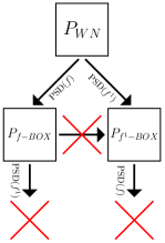
Figure 2: Orthogonal functions: If $f$ and $f^{1}$ are othogonal 1.) one cannot post-select them sequential with $P_{WN}$ as input and 2.) $P_{f-BOX}$ can’t be transformed into $P_{f^{1}-BOX}$ using any PSD.

b) Boolean compliments:

$P_{WN}$ can be prepared in many ways, which are indistinguishable from a device independent perspective. $P_{WN}$ is the center of the no-signaling polytope. So it could be broken down into infinite pairs of ’complementary’ correlations $P_{A,B},P^{\prime}_{A,B}$ such that,

$$P_{WN}=\frac{P_{A,B}+P^{\prime}_{A,B}}{2}.$$ (5)

If two functions $f$ and $f^{1}$are Boolean compliments that is $f=f^{1}\oplus 1$ then, 1) they must be orthogonal and, 2) they must produce complimentary correlations as output to $P_{WN}=\frac{P_{f-BOX}+P_{f^{1}-BOX}}{2}$. We can independently and simultaneously apply $f$ and $f^{1}$ as in principle we could have two post selection devices applied to $P_{WN}$ such that one accepts when $f=0$ and the other when $f=1$ (see FIG 3.).

Figure 3: Simultaneous application of PSD($f$) and PSD($f^{1}$), $f^{1}=f\oplus 1$. The outputs could again be mixed to form $P_{WN}$ that is $f\oplus f^{1}\oplus 1=0$ always holds.

II.3.2 Post-selection without the assumption.

In this we do not consider in general post selection to be efficient transformation in probability space. Post-selection in today’s world is basically a trial by trial evaluation of the input probability distribution wherein one simply accepts when $f=0$ (say) and ignores when $f=1$. It is easy to see that Post selection requires substantial amount of communication to get the input outputs of the two spatially separated parties to evaluate a Boolean function $f(x,y,u,v)$. In this context let us define an efficiency factor associated with the success probability of the post selection function given the communication required.

Definition 4. The efficiency of applying Post Selection function on the input probability distribution $P_{in}$ resulting in $P_{out}$ is given by $\eta^{P^{in}}_{f}\in(0,1)$. This efficiency factor is given by the success probability of the function $f$ to take the value $0$ i.e $\eta^{P^{in}}_{f}=P(f=0)$. Note that this efficiency is independent of the theory governing the boxes and only depends on $P_{in}$ and $f$.

III Implication of Post-selection as an assumption.

In this section we show that if we assume post selection to be a efficient transformation on the probability space, we observe the following surprising implications. This includes, 1) transforming no signaling probability distribution to signaling probability distribution, 2) solving NP Complete Problems 3) violation of Pigeon Hole Principle.

III.1 No signaling Theories to Signaling Theories via post-selection.

In this subsection we show that on application of fully efficient post selection function we can change no signaling probability distribution to signaling probability distribution.We white noise as input probability distribution because $P_{WN}(f=0)>0$ for all $f(x,y,u,v)$ and change it to signaling probability distribution. Similarly many other no signaling probability distributions that lie on the convex polytope are converted to signaling probability distributions on application of simple post selection described by Boolean functions. This inter convertibility is best represented by the schematic diagram given by the figure.

Let us consider the case where we take the input probability distribution as the white noise (probability distribution given in table 1) $P_{in}=P_{WN}$. One can obtain on application of a PSD($f$) a $P_{out}$, such that $P_{out}(f=0)=\sum_{f=0}P_{out}(u,v|x,y)=1$. The point $P_{out}$ is also referred to as $P_{f-BOX}$. In general for every Boolean function there exist a classical input output task (game) and a PSD($f$) that takes $P_{WN}$ to the correlation $P_{f-BOX}$ tailor made to win the task (with success probability = 1). This simply implies that using post-selection one can win all such tasks completely and violate all the physical principles associate with such tasks. The success probability of the associated the game $f$ can also be alternatively reported as the ”projection” of a point on the line joining $P_{f-BOX}$ and $P_{WN}$. On the basis of this observation we can formally categorize the set of $f$ (post-selection functions).

Signaling/No-signaling:

Definition 5. A function $f$ is called one-way(Alice-Bob) signaling iff,

$$I_{f-BOX}(A:B)>0.$$ (6)

Definition 6. A function $f$ is called one-way(Bob-Alice) signaling iff,

$$I_{f-BOX}(B:A)>0.$$ (7)

Definition 7. If both of the condition are met i.e $I_{f-BOX}(A:B)>0$ and $I_{f-BOX}(B:A)>0$ then $f$ is called both side signaling.

Definition 7. We say that a function is no-signaling when the following conditions are simultaneously met.

$$I_{f-BOX}(A:B)=0,$$ (8)

$$I_{f-BOX}(B:A)=0.$$ (9)

Local/non-local :

Definition 8. We say that a function $f$ is local if,

$$P_{f-BOX}(x.y=u\oplus y)\leq\frac{3}{4}.$$ (10)

Definition 9. We say that a function $f$ is non-local if,

$$P_{f-BOX}(x.y=u\oplus y)>\frac{3}{4}.$$ (11)

Interestingly there are only 5 non-local no-signaling functions. One of them is B-CHSH. Other functions are similar upto renaming to $f_{NL}$. The probability distribution for this non local box $P_{f_{NL}-BOX}(u,v|x,y)$ is shown in the TABLE VI.

		$x=0$		$x=1$
$P_{f_{NL}-BOX}(u,v|x,y)$		$u=0$	$u=1$	$u=0$	$u=1$
	$v=0$	$\frac{1}{4}$	$\frac{1}{4}$	$\frac{1}{2}$
$y=0$	$v=1$	$\frac{1}{4}$	$\frac{1}{4}$		$\frac{1}{2}$
	$v=0$	$\frac{1}{2}$			$\frac{1}{2}$
$y=1$	$v=1$		$\frac{1}{2}$	$\frac{1}{2}$

Table 6: Non Local Box: Probability distribution of $P_{f_{NL}-BOX}(u,v|x,y)$ with $P_{f_{NL}-BOX}(f_{B-CHSH}=0)=\frac{7}{8}$for binary inputs $x$ and $y$ and outputs $u$ and $v$. The empty boxes signifies the positions where $f_{NL}=1$ and can be taken as $0$.

In the FIG 4, we show a part of no signaling polytope and the transformation of the initial probability distribution $P_{in}=P_{WN}$ to various probability distributions with the application of post selection functions $f_{sig1}$, $f_{sig2}$, $f_{sig}$, $f_{B-CHSH}$, $f_{CTC}$. We take specific examples: $f_{sig1}:v\oplus x$, $f_{sig2}:u\oplus y$, $f_{sig}:(x\oplus v\oplus 1).(u\oplus y\oplus 1)\oplus 1$, $f_{B-CHSH}:x.y\oplus u\oplus v$, $f_{CTC}:y\oplus v$.

Figure 4: Transformation of Probability Distribution: In this schematic diagram the transformation of the initial probability distribution $P_{WN}$ to different output probability distribution on application of different post selection functions $f:f_{sig1},f_{sig2},f_{sig},f_{B-CHSH},f_{CTC}$ is shown.

.

In the TABLE VII we enlist down the signaling and no signaling possibilities (by evaluating $I(A:B)$ and $I(B:A)$ ). These post selection functions are $f_{sig1}$, $f_{sig2}$, $f_{sig}$, $f_{B-CHSH}$, $f_{CTC}$. The input probability distribution are $P_{WN}$, $P_{LV}$, $P_{SINGLET}$, $P_{PR-BOX}$, $P_{f_{NL}-BOX}$ (all no signaling probability distribution). We calculate each of the mutual information $I(A:B)$ and $I(B:A)$. In a nut shell this table gives a holistic view how the post selection when applied on an input probability distribution changes no signaling probability distributions to signaling probability distributions.

$f$	$P_{i}n$	$I(A:B)$	$I(B:A)$
$f_{sig1}$	$P_{WN}$	$1$	$0$
	$P_{LV}$	$1$	$0$
	$P_{SINGLET}$	$1$	$0.394553$
	$P_{PR-BOX}$	$1$	$\frac{1}{2}$
	$P_{f_{NL}-BOX}$	$1$	$\frac{1}{2}$
$f_{sig2}$	$P_{WN}$	$0$	$1$
	$P_{LV}$	$0$	$1$
	$P_{SINGLET}$	$0.394553$	$1$
	$P_{PR-BOX}$	$\frac{1}{2}$	$1$
	$P_{f_{NL}-BOX}$	$\frac{1}{2}$	$1$
$f_{sig}$	$P_{WN}$	$1$	$1$
	$P_{LV}$	$1$	$1$
	$P_{SINGLET}$	$1$	$1$
	$P_{PR-BOX}$	$1$	$1$
	$P_{f_{NL}-BOX}$	$1$	$1$
$f_{B-CHSH}$	$P_{WN}$	$0$	$0$
	$P_{LV}$	$0$	$0$
	$P_{SINGLET}$	$0$	$0$
	$P_{PR-BOX}$	$0$	$0$
	$P_{f_{NL}-BOX}$	$0$	$0$
$f_{CTC}$	$P_{WN}$	$0$	$0$
	$P_{LV}$	$0$	$0$
	$P_{SINGLET}$	$0.394553$	$0$
	$P_{PR-BOX}$	$\frac{1}{2}$	$0$
	$P_{f_{NL}-BOX}$	$\frac{1}{4}$	$0$

Table 7: Application of the Post Selection functions $f$: $f_{sig1}$, $f_{sig2}$, $f_{sig}$, $f_{B-CHSH}$, $f_{CTC}$ on Input No signaling probability distributions $P_{in}$: $P_{WN}$, $P_{LV}$, $P_{SINGLET}$, $P_{PR-BOX}$, $P_{f_{NL}-BOX}$

Few Specific Examples :

Apart from providing the previous table where we have shown the transition of a no signaling probability distributions to a signaling probability distributions on application of post selection functions; here also we provide few specific examples in TABLES VII, VIII, IX,X, XI with much more detailing.

• In TABLE VIII we provide an example where Alice to Bob signaling is taking place i.e $I(A:B)=1$. In this case we take the input probability distribution as the white noise $P_{WN}$ and the post selection function as $f_{sig1}$.

• In TABLE IX we provide an example where Bob to Alice signaling is taking place i.e $I(B:A)=1$. Here also we take the input probability distribution as the white noise $P_{WN}$ and this time the post selection function is $f_{sig2}$.

• In TABLE X we show the case where both way signaling is possible with the same input probability distribution $P_{WN}$ and the post signaling function as $f_{sig}$.

• In the next TABLE XI we take the input probability distribution as a convex combination of PR box and white noise i.e $P_{in}=cP_{PR-BOX}+(1-c)P_{WN}$ where $0<c<1$. In this case the post selection function is $f_{CTC}$ which when applied to $P_{in}$ we find the mutual information as $I(A:B)=\frac{1}{2}(1-\frac{1+c}{2}\log{\frac{1+c}{2}}+\frac{1-c}{2}\log{\frac{1-c}{2}})$. But $I(B:A)=0$ implying that there is only one-side signaling. Its interesting to note that it takes all other correlations on the line joining $P_{WN}$ and $P_{PR-BOX}$ to signaling.

• In TABLE XII we take the input probability distribution as $P_{in}=cP_{NL-BOX}+(1-c)P_{WN}$ where $0<c<1$. The post selection function $f_{CTC}$ is same as the previous case. The mutual information in this case is given by $I(A:B)=\frac{1}{4}(1-\frac{1+c}{2}\log{\frac{1+c}{2}}+\frac{1-c}{2}\log{\frac{1-c}{2}})$.

		$x=0$		$x=1$
$P_{f-BOX}(u,v|x,y)$		$u=0$	$u=1$	$u=0$	$u=1$
	$v=0$	$\frac{1}{2}$	$\frac{1}{2}$
$y=0$	$v=1$			$\frac{1}{2}$	$\frac{1}{2}$
	$v=0$	$\frac{1}{2}$	$\frac{1}{2}$
$y=1$	$v=1$			$\frac{1}{2}$	$\frac{1}{2}$

Table 8: Application of post selection function $f_{sig1}$ on $P_{WN}$: Alice to Bob signaling, $I(A:B)=1$.

		$x=0$		$x=1$
$P_{f-BOX}(u,v|x,y)$		$u=0$	$u=1$	$u=0$	$u=1$
	$v=0$	$\frac{1}{2}$		$\frac{1}{2}$
$y=0$	$v=1$	$\frac{1}{2}$		$\frac{1}{2}$
	$v=0$		$\frac{1}{2}$		$\frac{1}{2}$
$y=1$	$v=1$		$\frac{1}{2}$		$\frac{1}{2}$

Table 9: Application of post selection function $f_{sig2}$ on $P_{WN}$: Bob to Alice signaling, $I(B:A)=1$.

		$x=0$		$x=1$
$P_{f-BOX}(u,v|x,y)$		$u=0$	$u=1$	$u=0$	$u=1$
	$v=0$	$1$
$y=0$	$v=1$			$1$
	$v=0$		$1$
$y=1$	$v=1$				$1$

Table 10: Application of post selection function $f_{sig}$ on $P_{WN}$: Both side signaling, $I(A:B)=1$ and $I(B:A)=1$.

		$x=0$		$x=1$
$P_{f^{CTC}-BOX}(u,v|x,y)$		$u=0$	$u=1$	$u=0$	$u=1$
	$v=0$	$\frac{1+c}{2}$	$\frac{1-c}{2}$	$\frac{1+c}{2}$	$\frac{1-c}{2}$
$y=0$	$v=1$
	$v=0$
$y=1$	$v=1$	$\frac{1-c}{2}$	$\frac{1+c}{2}$	$\frac{1+c}{2}$	$\frac{1-c}{2}$

Table 11: Application of post selection function $f_{CTC}$ on $P_{in}=cP_{PR-BOX}+(1-c)P_{WN}$: Alice to Bob signaling.

		$x=0$		$x=1$
$P_{f^{CTC}-BOX}(u,v|x,y)$		$u=0$	$u=1$	$u=0$	$u=1$
	$v=0$	$\frac{1}{2}$	$\frac{1}{2}$	$\frac{1+p}{2}$	$\frac{1-p}{2}$
$y=0$	$v=1$
	$v=0$
$y=1$	$v=1$	$\frac{1-p}{2}$	$\frac{1+p}{2}$	$\frac{1+p}{2}$	$\frac{1-p}{2}$

Table 12: Application of post selection function $f_{CTC}$ on $P_{in}=cP_{NL-BOX}+(1-c)P_{WN}$: Alice to Bob signaling.

III.2 Post-selection, RP and NP-Completeness

$NP$ stands for “non deterministic polynomial time,” a term going back to the roots of complexity theory papadimitriou2003computational . Intuitively, it means that a solution to any search problem can be found and verified in polynomial time by a special (and quite unrealistic) sort of algorithm, called a non deterministic algorithm. Such an algorithm has the power of guessing correctly at every step. Incidentally, the original definition of $NP$ (and its most common usage to this day) was not as a class of search problems but as a class of decision problems. In other words $NP$ is set of all decision problems which can be verified, but not necessarily be solved, in polynomial time.

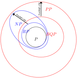
Figure 5: This figure describes the relationship between the complexity classes $P,RP,BQP,NP,PP$. $PostBQP=PP$(red) and $PostRP=NP$(blue).

Definition 10. A language $L$ is said to belong to class $NP$ iff for every $x\in L$, there exists a $y$, such that $\mid y\mid\leq p(\mid x\mid)$, for some polynomial $p$, and $L^{\prime}=\{(x,y):x\in L\}$ can be decided in polynomial time.

In other words, a problem is considered to be in the class $NP$, if for every true instance of the problem, there exists a proof of the answer, with polynomial bounded length, such that given the input and the proof, the proof can be verified in polynomial time. In complexity theory, the canonical $NP-complete$ problem, to which all problems of $NP$ can be reduced to, is $3SAT$, i.e. deciding whether a Boolean CNF formula with every $m$ clauses of size 3, over $n$ variables, is satisfy able or not. Therefore, if we can solve $3SAT$ in any framework, we can solve any NP problem in that framework. A common classical probability framework is defined by $RP$, which is the class of all problems which can be solved by a probabilistic Turi ng machine in polynomial time, such that error for No-instances is zero, and error for Yes-instances is less than $\frac{1}{2}$. While it is not known whether $RP$ is equal to $NP$ or not, it is known that $RP\subseteq NP$. However, in this section, we consider the post selection version of $RP$, and discuss its equivalence to $NP$.

Definition 11. A language $L$ is considered to be in class $PostRP$ iff there exists a probabilistic Turing Machine $M$, that for any input $x$, returns output $Q$ and a flag (on which one post selects) $P$ such that

1. $Pr(P=1)>0$,

2. For $x\notin L$, $Pr(Q=1\mid P=1)=0$,

3. For $x\in L$, $Pr(Q=1\mid P=1)\geq\frac{1}{2}$.

We now consider the randomness in the probabilistic Turing Machine explicitly, to make some observations about the nature of the language $L$. The machine $M$ can be interpreted to compute, in polynomial time, two functions $P$ and $Q$, given original input $x$ and a string of polynomially many random bits $r$ as inputs. Therefore, by converting the nonzero probabilities from the definition of Post RP to existential statements on the random string $r$, we get the following corresponding assertions:

1. $\forall x:\exists r:P(x,r)=1$,

2. $\forall x:x\notin L\implies\nexists r:Q(x,r)=1\wedge P(x,r)=1$,

3. $\forall x:x\in L\implies\exists r:Q(x,r)=1\wedge P(x,r)=1$.

Therefore, a proof scheme for such a problem directly follows from its probabilistic Turing machine. By assuming the random string $r$ as a proof of membership, a verifier can simply compute $P$ and $Q$ in polynomial time, and check whether both are equal to $1$. This scheme results in a membership proof, since

• For non-members, no such $r$ exists, hence no proof exists.

• For members (i.e. Yes-instances), there does exist a proof that can be verified in polynomial time.

Now we show that $NP\subseteq PostRP$ by constructing a probabilistic Turing Machine $M$ that can solve $3SAT$ in $PostRP$. We define $M$ as

1. Guess variable assignment $\sigma$, uniformly at random,

2. Check whether $\sigma$ satisfies the formula $\Phi$, and assign Q=1 if it does a) if No (i.e. Q=0), then assign P=1 with probability $\alpha$ b) if Yes (i.e. Q=1), then assign P=1 with probability $2^{n}\times\alpha$.

For a 3 SAT formula $\Phi$, let $0\leq s\leq 2^{n}$ denote the number of satisfying solutions. Thus $\Phi\in 3SAT\iff s>0$. Since the machine $M$ guesses an assignment and checks if it is a satisfying assignment, we know that if $s=0$ then $Pr(Q=1)=0$. Therefore we note that if $s=0$ and $\Phi\notin 3SAT$, then $Pr(P=1)$ is governed only by the case where $Q=0$, and thus equals $\alpha$. Therefore, $Pr(P=1)>0$. Also, since $Pr(Q=1)=0$, therefore $Pr(Q=1\bar{P}=1)=0$.

While, if $s>0$ and $\Phi\in 3SAT$, then $Pr(P=1)=\frac{(2^{n}-s)\alpha+s2^{n}\alpha}{2^{n}}>0$. Also since the assignments are guessed uniformly at random, $Pr(Q=1)=\frac{s}{2^{n}}>0$. Therefore,

$$Pr(Q=1\mid P=1) =\frac{Pr(P=1\mid Q=1)Pr(Q=1)}{Pr(P=1)}{}$$ (12)

$$=\frac{2^{n}\alpha\times s}{(2^{n}-s)\alpha+s2^{n}\alpha}{}$$

$$=\frac{2^{n}s}{2^{n}+(2^{n}-1)s}{}$$

$$>1/2.$$

Thus we show that the machine $M$ solves $3SAT$ as per Definitions 10, 11, thereby making $3SAT\in PostRP$, and it follows from $NP-completeness$ of $3SAT$ that $NP\subseteq PostRP$. We, thus, complete our proof of $NP=PostRP$. Post selection strengthens RP up till NP.

III.3 Violating Pigeon-Hole principle

One of the most simple yet fascinating principle of nature is the pigeonhole principle which captures the very essence of counting. In a way this principle tells us that if we put three pi- pigeons in two pigeonholes at least two of the pi- geons end up in the same hole. In other way round this implies that always there is a non-zero probability of finding any two pigeons in the same box. Recently in a work it was shown that in quantum mechanics this is not true. They found instances when three quantum particles are put in two boxes, yet no two particles are in the same box. Here in this section we show that post selection violates the pigeon hole principle independent of the theoretical setting.

Pigeon Hole principle: If you put three pigeons in two pigeonholes at least two of the pigeons end up in the same hole.

Violation of Pigeon Hole principle: Finding an instance when three pigeons are put in two box where no two pigeons are in the same box.

Claim: Our claim is to show that post selection is alone responsible for the violation of the principle independent of any theoretical setting.

III.3.1 Modeling and the skeleton.

We treat the pigeons as general probability distributions or black boxes with fixed inputs and outputs. Let us take three pigeons $A,B,C$. Here we are concerned about only two properties of the pigeons: 1)color(Red or Blue) and 2)hole (Left or Right). Here two questions are allowed to ask to each pigeon. These questions are denoted by $x,y,z\in\{0,1\}$ for three pigeons $A,B,C$ respectively. Consequently they are allowed to give binary answers(outputs) $u,v,w\in\{0,1\}$ respectively. If input $x=0$ we need the answer to say the color of $A$ which could be $u=0$ (say Red) or $u=1$ (say Blue) and similarly if $x=1$ we want to know in which hole $A$ is i.e. $u=0$ (say Left) and $u=1$ (say Right). Similar questions and answers also hold for other two pigeons $B$ and $C$.

These boxes are completely described by the associated probabilities $P_{A,B,C}(u,v,w|x,y,z)$. To obtain individual probabilities like $P_{A}(u|x)$ and pair wise probabilities like $P_{A<B}(u,v|x,y)$ one can simply trace(sum) out other systems. For example,

$$P_{A,B}(u,v|x,y)=\frac{\sum_{w,z}{P_{A,B,C}(u,v,w|x,y,z)}}{2}.$$ (13)

III.3.2 The Pre-selection.

Here we preselect the initial probability distribution as the uniform probability distribution of white noise i.e, $P_{A,B,C}(u,v,w|x,y,z)=\frac{1}{8}$ for all $u,v,w,x,y,z\in\{0,1\}$. Now we make our basic assumption,

Assumption: The pigeons are same upto renaming.

This allows us to reduce the number to two, $P_{A,B}=P_{WN}$ such that $P(u,v|x,y)=\frac{1}{4}$ for all $u,v,x,y\in\{0,1\}$.

III.3.3 The Post-selection.

Let $f_{final}=(x\oplus 1).(y\oplus 1).(z\oplus 1).(u\oplus 1).(v\oplus 1).(w\oplus 1)\oplus 1$ be the PSD governing function. The output probability distribution $P_{out}$ is simply $P(u=0,v=0,w=0|x=0,y=0,z=0)=1$and $P(u,v,w|x,y,z)=0$ for all other cases.

Notice that this function selects the pigeons with the same color, it has nothing to do with the hole in which they are present and we start with a White-Noise distribution, therefore the pigeon hole principle is still valid.

III.3.4 The question.

We pre-select and post-select the same no-violation probability distributions as described above. We need only find a possible path where the probability of the pigeons being in the same hole is zero. We question the path that could have been taken in between. Our question is whether a function $f_{1}$ could have been applied in between or not? In other words, looking only at the final post-selection we need to find whether $P_{WN}$ could have passed through $P_{f_{1}-BOX}$ or not in world with the assumption.

		$x=0$		$x=1$
$P_{f_{1}-BOX}(u,v|x,y)$		$u=0$	$u=1$	$u=0$	$u=1$
	$v=0$		$\frac{1}{2}$		$\frac{1}{2}$
$y=0$	$v=1$	$\frac{1}{2}$		$\frac{1}{2}$
	$v=0$	$\frac{1}{2}$		$\frac{1}{2}$
$y=1$	$v=1$		$\frac{1}{2}$		$\frac{1}{2}$

Table 13: $P_{f_{1}-BOX}$ and $P_{f_{1}-BOX}(f_{B-CHSH}=\frac{3}{4})$

Notice $f_{final}$ and $f_{1}$ are orthogonal PS functions. Let $f_{2}$ be a Boolean complement of $f_{1}$ and can be applied simultaneously.

		$x=0$		$x=1$
$P_{f_{2}-BOX}(u,v|x,y)$		$u=0$	$u=1$	$u=0$	$u=1$
	$v=0$	$\frac{1}{2}$		$\frac{1}{2}$
$y=0$	$v=1$		$\frac{1}{2}$		$\frac{1}{2}$
	$v=0$		$\frac{1}{2}$		$\frac{1}{2}$
$y=1$	$v=1$	$\frac{1}{2}$		$\frac{1}{2}$

Table 14: $P_{f_{2}-BOX}$ and $P_{f_{2}-BOX}(f_{B-CHSH}=\frac{3}{4})$

Notice $f_{2}$ (see FiG 6) is not orthogonal to $f_{final}$ and therefore is a valid path. Notice after application of $f_{2}$ pigeons would necessarily be in different holes. So using post-selection one can violate the pigeon hole between to non-violating states.

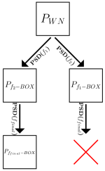
Figure 6: This figure describes theory independent violation of the pigeon hole principle. $f_{1},f_{final}$ are orthogonal as $P_{{f_{1}}-BOX}(f_{final}=0)=0$. So one cannot post-select $f_{final}$ after $f_{1}$. On the other hand $f_{2}=f_{1}\oplus 1$, implying $f_{2},f_{final}$ are not orthogonal and hence a valid path in which any two pigeons must be in different holes.

IV Post-selection without the assumption.

In this section, we associate an efficiency factor $\eta^{f}_{P_{in}}$ with each of these transformations (described by Boolean function $f$) for a given input probability distribution $P_{in}$ . We consider the examples used in the previous section and calculate the efficiency factor. In the next subsection we discuss the role of post-selection from an adversarial perspective and find out the robust bounds on maximum efficiency required for simulating non local correlations from an adversarial perspective.

IV.1 Evaluating Efficiency Factor

In a world without the assumption the loss of trial(efficiency) is the key factor. In TABLE XV we provide the device independent efficiency ($\eta^{P_{in}}_{f}$) for a given post selection function $f$ and input probability distribution $P_{in}$.

$f$	$P_{i}n$	$\eta^{P_{in}}_{f}$
$f_{sig1}$	$P_{WN}$	$\frac{1}{2}$
	$P_{LV}$	$\frac{1}{2}$
	$P_{SINGLET}$	$\frac{1}{2}$
	$P_{PR-BOX}$	$\frac{1}{2}$
	$P_{f_{NL}-BOX}$	$\frac{1}{2}$
$f_{sig2}$	$P_{WN}$	$\frac{1}{2}$
	$P_{LV}$	$\frac{1}{2}$
	$P_{SINGLET}$	$\frac{1}{2}$
	$P_{PR-BOX}$	$\frac{1}{2}$
	$P_{f_{NL}-BOX}$	$\frac{1}{2}$
$f_{sig}$	$P_{WN}$	$\frac{1}{4}$
	$P_{LV}$	$\frac{1}{4}$
	$P_{SINGLET}$	$0.1616$
	$P_{PR-BOX}$	$\frac{1}{8}$
	$P_{f_{NL}-BOX}$	$\frac{1}{16}$
$f_{B-CHSH}$	$P_{WN}$	$\frac{1}{2}$
	$P_{LV}$	$\frac{3}{4}$
	$P_{SINGLET}$	$\frac{2+\sqrt{2}}{4}$
	$P_{PR-BOX}$	$1$
	$P_{f_{NL}-BOX}$	$\frac{7}{8}$
$f_{CTC}$	$P_{WN}$	$\frac{1}{2}$
	$P_{LV}$	$\frac{1}{2}$
	$P_{SINGLET}$	$\frac{1}{2}$
	$P_{PR-BOX}$	$\frac{1}{2}$
	$P_{f_{NL}-BOX}$	$\frac{1}{2}$

Table 15: In this Table we enlist down the respective efficiency factor for post selection functions $f$: $f_{sig1}$, $f_{sig2}$, $f_{sig}$, $f_{B-CHSH}$, $f_{CTC}$ and a given input probability distributions $P_{in}$: $P_{WN}$, $P_{LV}$, $P_{SINGLET}$, $P_{PR-BOX}$, $P_{f_{NL}-BOX}$

One can notice that such post-selection are fairly costly. Post-selection in real world does not alter the underlying probability distribution. As a consequence there is no violation of the Pigeon hole principle in the classical world. While it is not known yet whether $RP=NP$, it is however interesting to note why the technique employed here does not suffice to prove it. But, even with the given construction, one would require an expected $\frac{1}{Pr(P=1)}$, which is exponential, runs of the machine to get a selective run. Guessing boolean assignments at random and then verifying whether the formula satisfies it, has a probability of success, in single run, $\frac{s}{2^{n}}$. Thus, for such a method to have a probability greater than $\frac{1}{2}$, one would have to repeat the experiment exponential number of times.

Next we re discuss two important properties of post selection function namely orthogonality and Boolean compliments in terms of efficiency factor $\eta^{P_{in}}_{f}$.

a) Sequential application and (semi-)orthogonal functions.

Start again with $P_{WN}$, the drop in efficiency on sequential application of two functions $f$ (say first) and (then) $f_{1}$ are given by,

$$\eta^{P_{WN}}_{f,f^{1}}=P_{WN}((f=0)\wedge(f^{1}=0)).$$ (14)

If $f$ and $f_{1}$ are orthogonal then,

$$\eta^{P_{WN}}_{f,f^{1}}=0.$$ (15)

Definition 12. Two functions are semi orthogonal if,

$$\eta^{P_{WN}}_{f,f^{1}}<\eta^{P_{WN}}_{f}\eta^{P_{f_{BOX}}}_{f^{1}}.$$ (16)

Definition 13. Two functions are $f$ and $f^{1}$ are non orthogonal if

$$\eta^{P_{WN}}_{f,f^{1}}=\eta^{P_{WN}}_{f}\eta^{P_{f_{BOX}}}_{f^{1}},$$ (17)

which is the case with $f_{2}$ and $f_{final}$.

b) Boolean Compliments.

If two functions $f$ and $f^{1}$are Boolean compliments that is $f=f^{1}\oplus 1$ then,

1. : As $P((f=0)\wedge(f^{1}=0))=0$,

   $$\eta^{P_{WN}}_{f,f^{1}}=0.$$ (18)

2. As $P((f=0)\vee(f^{1}=0))=1$

   $$\eta^{P_{WN}}_{f}+\eta^{P_{WN}}_{f^{1}}=1.$$ (19)

We can simultaneously apply $f$ and $f^{1}$ as in principle we could have two PSD applied to $P_{WN}$ such that one accepts when $f=0$ and the other when $f=1$.

IV.2 From an adversarial perspective.

From an adversarial perspective, faking correlations, in particular Bell violation is of great importance. The fact that Eve cannot fake (simulate) non-local correlations (at $\eta=1$ using post-selection leads to device independently secure self assessment, QKD (Quantum Key Distribution scheme), randomness expansion and so on. However at lower efficiency a Eve could apply post-selection (denial of service attack) and fake correlations ( Bell violation in particular ). We provide a (optimal) protocol for potential Eves dropper and study the relationship between input/output (actual/apparent)probability distribution and the device independent efficiency factor associated with them. As a result with provide robust bounds on minimum efficiency for non-locality of singlet statistics and for $\epsilon$ bell violation.

In general lets say Eve starts with $P_{in}$ with some $P_{in}(f=0)$ and wants to simulate $P_{out}(f=0)>P_{in}(f=0)$. She can do this by following the protocol,

1. Whenever $f=0$ accept the trial.

2. Whenever $f=1$, with $p\in\{0,1\}$ probability accept the trial.

Here the efficiency $\eta^{P_{WN}}_{x.y\oplus u\oplus v}=\frac{1+p}{2}$, so $P_{out}(f=0)=\frac{1}{1+p}$. So Eve can cheat Alice and Bob to believe that they share a correlation with $P_{out}(f=0)$ at maximum efficiency,

$$\eta^{P_{in}}_{f}=\frac{P_{in}(f=0)}{P_{out}(f=0)}.$$ (20)

The malicious Eve wants to simulate the statistics of the singlet quantum state in a Bell experiment. We already know it is impossible to do this at $\eta^{P^{in}}_{f}=1$ or the case of perfect (detectors) devices. However at lower $\eta^{P^{in}}_{f}\leq 1$ it possible to apply quantum Bell violation. So Eve can cheat Alice and Bob to believe that they share a singlet state with an efficiency factor at most equal to

$$\eta^{P^{WN}}_{x.y\oplus u\oplus v}=\frac{1}{2max_{Q}(P^{out}_{B-CHSH})}=\frac{2}{2+\sqrt[]{2}}=0.585786.$$ (21)

$P_{WN}$ cannot simulate singlet statistics at efficiency above $\eta^{P^{WN}}_{x.y\oplus u\oplus v}$. How ever Eve could use other classical correlations such as $P_{in}=max(P^{B-CHSH}_{LV})=\frac{3}{4}$. She follows the same protocol. Now the efficiency $\eta^{P_{in}}_{x.y\oplus u\oplus v}=\frac{3+p}{4}$, so $P^{out}_{B-CHSH}=\frac{3}{3+p}$. So Eve can cheat Alice and Bob to believe that they share a singlet state with

$$\eta^{P_{LV}}_{x.y\oplus u\oplus v}=\frac{3}{4max_{Q}(P^{out}_{B-CHSH})}=\frac{3}{2+\sqrt[]{2}}=0.87867$$ (22)

$P_{LV}$ cannot simulate singlet statistics at efficiency above $\eta^{P^{LV}}_{x.y\oplus u\oplus v}$, so the singlet statistics can guarantee Bell-Violation at higher efficiency. In general for $\epsilon\in(0,\frac{1}{4})$ one requires,

$$\eta^{P_{LV}}_{x.y\oplus u\oplus v}=\frac{\frac{3}{4}}{\frac{3}{4}+\epsilon}.$$ (23)

In TABLE XVI we write down the bounds of the efficiency factor $\eta^{P_{in}}_{f}$ for a given input probability distribution $P_{in}$, post selection function $f$ and the output probability distribution $P_{out}$.

$f$	$P_{in}$	$P_{out}$	$P_{out}(f_{B-CHSH}=0)$	$\eta^{P_{in}}_{f}$
$f_{B-CHSH}$	$P_{WN}$	$P_{SINGLET}$	$0.85355339059$	$0.585786$
		$P_{PR-BOX}$	$1$	$\frac{1}{2}$
	$P_{LV}$	$P_{SINGLET}$	$0.85355339059$	$0.87867$
		$P_{PR-BOX}$	$1$	$\frac{3}{4}$

Table 16: Bounds on $\eta^{P_{in}}_{f}$ for input probability distribution $P_{in}$, output probability distribution $P_{out}$ and post selection function $f$.

References

- (1) D. Hilbert, J. v. Neumann, and L. Nordheim, “Über die grundlagen der quantenmechanik,” Mathematische Annalen, vol. 98, no. 1, pp. 1–30, 1928.
- (2) A. Einstein, B. Podolsky, and N. Rosen, “Can quantum-mechanical description of physical reality be considered complete?,” Physical review, vol. 47, no. 10, p. 777, 1935.
- (3) E. Santos, “Critical analysis of the empirical tests of local hidden-variable theories,” Physical review A, vol. 46, no. 7, p. 3646, 1992.
- (4) L. Ballentine, “Einstein’s interpretation of quantum mechanics,” American Journal of Physics, vol. 40, no. 12, pp. 1763–1771, 1972.
- (5) M. Tegmark and J. A. Wheeler, “100 years of the quantum,” arXiv preprint quant-ph/0101077, 2001.
- (6) J. S. Bell et al., “On the einstein-podolsky-rosen paradox,” Physics, vol. 1, no. 3, pp. 195–200, 1964.
- (7) D. Home and F. Selleri, “Bell’s theorem and the epr paradox,” La Rivista del Nuovo Cimento, vol. 14, no. 9, pp. 1–95, 1991.
- (8) G.-P. Guo, C.-F. Li, J. Li, and G.-C. Guo, “Scheme for the preparation of multiparticle entanglement in cavity qed,” Physical Review A, vol. 65, no. 4, p. 042102, 2002.
- (9) C. H. Bennett, G. Brassard, C. Crépeau, R. Jozsa, A. Peres, and W. K. Wootters, “Teleporting an unknown quantum state via dual classical and einstein-podolsky-rosen channels,” Physical review letters, vol. 70, no. 13, p. 1895, 1993.
- (10) S. Adhikari, A. Majumdar, and N. Nayak, “Teleportation of two-mode squeezed states,” Physical Review A, vol. 77, no. 1, p. 012337, 2008.
- (11) N. Gisin, G. Ribordy, W. Tittel, and H. Zbinden, “Quantum cryptography,” Reviews of modern physics, vol. 74, no. 1, p. 145, 2002.
- (12) H.-K. Lo, M. Curty, and B. Qi, “Measurement-device-independent quantum key distribution,” Physical review letters, vol. 108, no. 13, p. 130503, 2012.
- (13) A. Ekert and R. Renner, “The ultimate physical limits of privacy,” Nature, vol. 507, no. 7493, pp. 443–447, 2014.
- (14) L. Masanes, S. Pironio, and A. Acin, “Secure device-independent quantum key distribution with causally independent measurement devices,” Nature communications, vol. 2, p. 238, 2011.
- (15) A. Acín, N. Brunner, N. Gisin, S. Massar, S. Pironio, and V. Scarani, “Device-independent security of quantum cryptography against collective attacks,” Physical Review Letters, vol. 98, no. 23, p. 230501, 2007.
- (16) M. Hillery, V. Bužek, and A. Berthiaume, “Quantum secret sharing,” Physical Review A, vol. 59, no. 3, p. 1829, 1999.
- (17) R. Colbeck and A. Kent, “Private randomness expansion with untrusted devices,” Journal of Physics A: Mathematical and Theoretical, vol. 44, no. 9, p. 095305, 2011.
- (18) S. Pironio, A. Acín, S. Massar, A. B. de La Giroday, D. N. Matsukevich, P. Maunz, S. Olmschenk, D. Hayes, L. Luo, T. A. Manning, et al., “Random numbers certified by bell’s theorem,” Nature, vol. 464, no. 7291, pp. 1021–1024, 2010.
- (19) I. Chakrabarty, “Secret broadcasting of w-type state,” International Journal of Quantum Information, vol. 7, no. 02, pp. 559–565, 2009.
- (20) S. Adhikari, I. Chakrabarty, and P. Agrawal, “Probabilistic secret sharing through noisy quantum channel,” Quantum Information & Computation, vol. 12, no. 3-4, pp. 253–261, 2012.
- (21) C. H. Bennett and S. J. Wiesner, “Communication via one-and two-particle operators on einstein-podolsky-rosen states,” Physical review letters, vol. 69, no. 20, p. 2881, 1992.
- (22) C. H. Bennett, D. P. DiVincenzo, P. W. Shor, J. A. Smolin, B. M. Terhal, and W. K. Wootters, “Remote state preparation,” Physical Review Letters, vol. 87, no. 7, p. 077902, 2001.
- (23) A. K. Pati, “Minimum classical bit for remote preparation and measurement of a qubit,” Physical Review A, vol. 63, no. 1, p. 014302, 2000.
- (24) S. Chatterjee, S. Sazim, and I. Chakrabarty, “No broadcasting of quantum correlation,” arXiv preprint arXiv:1411.4397, 2014.
- (25) S. Adhikari and B. Choudhury, “Broadcasting of three-qubit entanglement via local copying and entanglement swapping,” Physical Review A, vol. 74, no. 3, p. 032323, 2006.
- (26) S. Sazim, I. Chakrabarty, C. Vanarasa, and K. Srinathan, “Retrieving and routing quantum information in a quantum network,” arXiv preprint arXiv:1311.5378, 2013.
- (27) E. S. Fry and R. C. Thompson, “Experimental test of local hidden-variable theories,” Physical Review Letters, vol. 37, no. 8, p. 465, 1976.
- (28) S. J. Freedman and J. F. Clauser, “Experimental test of local hidden-variable theories,” Physical Review Letters, vol. 28, no. 14, p. 938, 1972.
- (29) A. Fine, “Hidden variables, joint probability, and the bell inequalities,” Physical Review Letters, vol. 48, no. 5, p. 291, 1982.
- (30) B. M. Terhal, “Bell inequalities and the separability criterion,” Physics Letters A, vol. 271, no. 5, pp. 319–326, 2000.
- (31) J. M. Knight and L. Vaidman, “Weak measurement of photon polarization,” Physics Letters A, vol. 143, no. 8, pp. 357–361, 1990.
- (32) C. Ferrie and J. Combes, “How the result of a single coin toss can turn out to be 100 heads,” Physical review letters, vol. 113, no. 12, p. 120404, 2014.
- (33) Y. Aharonov, F. Colombo, S. Popescu, I. Sabadini, D. C. Struppa, and J. Tollaksen, “The quantum pigeonhole principle and the nature of quantum correlations,” arXiv preprint arXiv:1407.3194, 2014.
- (34) C. Branciard, “Detection loophole in bell experiments: How postselection modifies the requirements to observe nonlocality,” Physical Review A, vol. 83, no. 3, p. 032123, 2011.
- (35) C. H. Bennett and R. Landauer, “The fundamental physical limits of computation,” Scientific American, vol. 253, no. 1, pp. 48–56, 1985.
- (36) S. Lloyd, “Ultimate physical limits to computation,” Nature, vol. 406, no. 6799, pp. 1047–1054, 2000.
- (37) S. Aaronson, “Limits on efficient computation in the physical world,” arXiv preprint quant-ph/0412143, 2004.
- (38) Y. Aharonov, D. Z. Albert, and L. Vaidman, “How the result of a measurement of a component of the spin of a spin-1/2 particle can turn out to be 100,” Physical review letters, vol. 60, no. 14, p. 1351, 1988.
- (39) Y. Aharonov and L. Vaidman, “Properties of a quantum system during the time interval between two measurements,” Physical Review A, vol. 41, no. 1, p. 11, 1990.
- (40) L. Lydersen, C. Wiechers, C. Wittmann, D. Elser, J. Skaar, and V. Makarov, “Hacking commercial quantum cryptography systems by tailored bright illumination,” Nature photonics, vol. 4, no. 10, pp. 686–689, 2010.
- (41) S. Aaronson, “Guest column: Np-complete problems and physical reality,” ACM Sigact News, vol. 36, no. 1, pp. 30–52, 2005.
- (42) S. Aaronson, “Quantum computing, postselection, and probabilistic polynomial-time,” Proceedings of the Royal Society A: Mathematical, Physical and Engineering Science, vol. 461, no. 2063, pp. 3473–3482, 2005.
- (43) J. Conway and S. Kochen, “The free will theorem,” Foundations of Physics, vol. 36, no. 10, pp. 1441–1473, 2006.
- (44) M. Pawłowski, T. Paterek, D. Kaszlikowski, V. Scarani, A. Winter, and M. Żukowski, “Information causality as a physical principle,” Nature, vol. 461, no. 7267, pp. 1101–1104, 2009.
- (45) T. H. Yang, M. Navascués, L. Sheridan, and V. Scarani, “Quantum bell inequalities from macroscopic locality,” Physical Review A, vol. 83, no. 2, p. 022105, 2011.
- (46) C. H. Papadimitriou, Computational complexity. John Wiley and Sons Ltd., 2003.