Microwave Background Polarization as a Probe of Large-Angle Correlations

Abstract

Two-point correlation functions of cosmic microwave background polarization provide a physically independent probe of the surprising suppression of correlations in the cosmic microwave background temperature anisotropies at large angular scales. We investigate correlation functions constructed from both the Q and U Stokes parameters and from the E and B polarization components. The dominant contribution to these correlation functions comes from local physical effects at the last scattering surface or from the epoch of reionization at high redshift, so all should be suppressed if the temperature suppression is due to an underlying lack of correlations in the cosmological metric perturbations larger than a given scale. We evaluate the correlation functions for the standard $\Lambda$CDM cosmology constrained by the observed temperature correlation function, and compute statistics characterizing their suppression on large angular scales. Future full-sky polarization maps with minimal systematic errors on large angular scales will provide strong tests of whether the observed temperature correlation function is a statistical fluke or reflects a fundamental shortcoming of the standard cosmological model.

I Introduction

Two seasons of observational data from the Planck satellite have given us the most precise measurement of temperature fluctuations in the Cosmic Microwave Background on the full sky to date Ade:2013zuv ; Adam:2015rua ; Planck:2015xua . These observations appear to fit well within the standard picture of our Universe – Lambda Cold Dark Matter ($\Lambda$CDM). It did, however confirm several anomalous features in the temperature fluctuations Ade:2013nlj , which had first been hinted at with the COBE-DMR satellite Bennett:1996ce and were later highlighted in the WMAP data releases Spergel:2003cb . These anomalies exist overwhelmingly at the largest scales of the temperature power spectrum, $C^{TT}_{\ell}$, with several interesting features appearing at multipoles $\ell\lesssim 30$. One feature, the lack of two-point correlation at angular separations of $60^{\circ}$ and above, has garnered much attention recently Copi:2010na ; Copi:2008hw . With decades of temperature measurements in hand, we know that this lack of correlation occurs only $0.03-0.1$ per cent of the time in $\Lambda$CDM realizations.

These large scales are also where cosmic variance, rather than statistical errors, is the limiting factor in our ability to compare the observed value of $C_{\ell}^{TT}$ to its theoretical value. This means that additional measurements of the temperature fluctuations will not help us make more definitive statements about the nature of the lack of correlation, and whether it is a statistical fluke within our cosmological model or due to unknown physics. Work has been done recently to quantify the viability of using cross correlations of temperature with E-mode polarization Copi:2013zja and the lensing potential $\varphi$ Yoho:2013tta to test this “fluke hypothesis.”

Correlations of CMB polarization itself, outside of just cross correlations with the temperature observations, are a natural next step in determining the nature of the lack of temperature correlation seen at large angles. A feature that is required for a real-space correlation function is for the field to be calculated using only local operators on directly observed $Q$ and $U$ polarization maps. The very nature of a correlation function that has a clearly defined physical interpretation depends on points on the sky being determined independently of each other (i.e. locally).

To accomplish this, we calculate two sets of polarization correlation functions: $Q$ and $U$ auto-correlations along with $\hat{E}({\bf\hat{n}})$ and $\hat{B}({\bf\hat{n}})$ auto-correlations. These have a number of properties that make them unique tests of large-angle correlation suppression, such as contributions from the reionization bump that appear in polarization power spectra at $\ell\lesssim 10$ that dominate the large-angle $Q$ and $U$ functions. The local E- and B-mode correlations are instead dominated by large multipoles at large angles, and have small contributions from reionization which makes them a cleaner test of physics at the last scattering surface. In this work we present the local $C^{\hat{E}\hat{E}}(\theta)$ and $C^{\hat{B}\hat{B}}(\theta)$, along with $C^{QQ}(\theta)$ and $C^{UU}(\theta)$, and show distributions for the corresponding $S_{1/2}$ statistic for each. These results are drawn using constrained temperature realizations, meaning they are consistent with the observed power spectrum within instrumental errors and have a cut-sky $S_{1/2}$ at least as small as our cut-sky measurement.

This paper is organized as follows: in Section II we present the theoretical background for $C(\theta)$ and a commonly discussed statistic $S_{1/2}$, in Section III we discuss our calculation of the error based on next-generation satellite specifications as well as the lowest possible expected instrument-limited value of $S_{1/2}$, in Section IV we present the local E- and B-mode correlation functions, in Section V we show auto-correlation functions for Q and U Stokes parameters, and in Section VI we present our conclusions and discuss possibilities for future work.

II Background

II.1 Temperature Correlation Function and Statistics

The information contained in CMB temperature fluctuations is often represented in harmonic space by decomposing them in terms of spherical harmonics and their coefficients,

$$\frac{\Delta T({\bf\hat{n}})}{T_{o}}\equiv\Theta({\bf\hat{n}})=\sum_{\ell,m}a^{T}_{\ell m}Y_{\ell m}({\bf\hat{n}}),$$ (1)

with the temperature power spectrum being constructed from the $a_{\ell m}$ coefficients:

$$\langle a^{T}_{\ell m}a^{T*}_{\ell^{\prime}m^{\prime}}\rangle=\delta_{\ell\ell^{\prime}}\delta_{mm^{\prime}}C^{TT}_{\ell}$$ (2)

In real space, the CMB temperature fluctuations, $\Theta({\bf\hat{n}})$, can be represented as a two-point correlation function averaged over the sky at different angular separations:

$$C^{TT}(\theta)=\overline{\Theta({\bf\hat{n}_{1}})\Theta({\bf\hat{n}_{2}})}\quad{\mathrm{with}}\quad{\bf\hat{n}_{1}}\cdot{\bf\hat{n}_{2}}=\cos\theta.$$ (3)

This is an estimator of the quantity $C^{TT}(\theta)=\langle\Theta({\bf\hat{n}_{1}})\Theta({\bf\hat{n}_{2}})\rangle$, where the angle brackets represent an ensemble average. The sky average over the angular separation can be expanded in a Legendre series,

$$C^{TT}(\theta)=\sum_{\ell}\frac{2\ell+1}{4\pi}\,C_{\ell}^{TT}P_{\ell}(\cos\theta),$$ (4)

where the $C_{\ell}$ on the right-hand side of Eq. (4) are the pseudo-$C_{\ell}$ temperature power spectrum values.

The $S_{1/2}$ statistic was defined by the WMAP team to quantify the lack of angular correlation seen in temperature maps Spergel:2003cb :

$$S_{1/2}^{TT}\equiv\int_{-1}^{1/2}{\mathrm{d}}(\cos\theta)[C^{TT}(\theta)]^{2}.$$ (5)

The expression for $S_{1/2}$ can be written conveniently in terms of the temperature power spectrum and a coupling matrix $I_{\ell\ell^{\prime}}$,

$$S_{1/2}^{TT}=\sum_{\ell=2}^{\ell_{\mathrm{m}ax}}C_{\ell}^{TT}{I}_{\ell\ell^{\prime}}C_{\ell^{\prime}}^{TT}.$$ (6)

A full expression of the $I_{\ell\ell^{\prime}}$ matrix can be found in Appendix B of (Copi:2008hw, ). The $C_{\ell}$ fall sharply and higher order modes have a negligable contribution to the statistic, so choice of an appropriately large value of $\ell_{\mathrm{max}}$ in Eq. (5) will ensure that the result is not affected by including additional higher-$\ell$ terms.

II.2 Stokes $Q$ and $U$ Correlation Functions and Statistics

Linear polarization is typically described by two quantities: the $Q$ and $U$ Stokes parameters in real space, and E-modes and B-modes in harmonic space. In real space, $C^{QQ}(\theta)=\langle{Q_{r}({\bf\hat{n}_{1}})Q_{r}({\bf\hat{n}_{2}})}\rangle$ and $C^{UU}(\theta)=\langle U_{r}({\bf\hat{n}_{1}})U_{r}({\bf\hat{n}_{2}})\rangle$ are the $Q$ and $U$ correlation functions, where $Q_{r}({\bf\hat{n}})$ and $U_{r}({\bf\hat{n}})$ are the Stokes parameters defined with respect to the great arc connecting ${\bf\hat{n}_{1}}$ and ${\bf\hat{n}_{2}}$ Kamionkowski:1996zd . $Q({\bf\hat{n}})$ and $U({\bf\hat{n}})$ fields on the sphere are defined such that they are connected by a great arc of constant $\phi$. In practice, the correlation functions are calculated as an average over pixels separated by an angle $\theta$:

$$C^{QQ}(\theta) =\overline{Q_{r}({\bf\hat{n}_{1}})Q_{r}({\bf\hat{n}_{2}})},$$

$$C^{UU}(\theta) =\overline{U_{r}({\bf\hat{n}_{1}})U_{r}({\bf\hat{n}_{2}})}.$$ (7)

The decomposition of polarization into spin-2 spherical harmonics is done with a linear combination of the Stokes parameters,

$$\left(Q({\bf\hat{n}})\pm\mathrm{i}U({\bf\hat{n}})\right)=\sum_{\ell m}\;{}_{\pm 2}a^{P}_{\ell m}\;{}_{\pm 2}Y_{\ell m}({\bf\hat{n}}).$$ (8)

The standard E- and B-mode coefficients are combinations of the spin-2 harmonic coefficients,

$$a_{\ell m}^{B} =\frac{\mathrm{i}}{2}\left[{}_{2}a^{P}_{\ell m}-\;_{-2}a^{P}_{\ell m}\right]$$

$$a_{\ell m}^{E} =-\frac{1}{2}\left[{}_{2}a^{P}_{\ell m}+\;_{-2}a^{P}_{\ell m}\right],$$ (9)

and the E- and B-mode power spectra are defined as

$$\langle a^{E}_{\ell m}{a^{E}}^{*}_{\ell^{\prime}m^{\prime}}\rangle =\delta_{\ell\ell^{\prime}}\delta_{mm^{\prime}}C^{EE}_{\ell}$$

$$\langle a^{B}_{\ell m}{a^{B}}^{*}_{\ell^{\prime}m^{\prime}}\rangle =\delta_{\ell\ell^{\prime}}\delta_{mm^{\prime}}C^{BB}_{\ell}.$$ (10)

Using these equations, we can construct $C^{QQ}(\theta)$ and $C^{UU}(\theta)$ from $C_{\ell}^{BB}$ and $C_{\ell}^{EE}$ Kamionkowski:1996ks :

$$C^{QQ}(\theta) =-\sum_{\ell}\frac{2\ell+1}{4\pi}\left(\frac{2(\ell-2)!}{(\ell+2)!}\right)\times$$

$$\left[C_{\ell}^{EE}G_{\ell 2}^{+}(\cos\theta)+C_{\ell}^{BB}G_{\ell 2}^{-}(\cos\theta)\right]$$

$$C^{UU}(\theta) =-\sum_{\ell}\frac{2\ell+1}{4\pi}\left(\frac{2(\ell-2)!}{(\ell+2)!}\right)\times$$

$$\left[C_{\ell}^{EE}G_{\ell 2}^{-}(\cos\theta)+C_{\ell}^{BB}G_{\ell 2}^{+}(\cos\theta)\right],$$ (11)

where

$$G_{\ell m}^{+}(\cos\theta) =-\left(\frac{\ell-m^{2}}{\sin^{2}\theta}+\frac{\ell(\ell-1)}{2}P_{\ell}^{m}(\cos\theta)\right)$$

$$+(\ell+m)\frac{\cos\theta}{\sin^{2}\theta}P_{\ell-1}^{m}(\cos\theta),$$

$$G_{\ell m}^{-}(\cos\theta) =\frac{m}{\sin^{2}\theta}\left((\ell-1)\cos\theta P_{\ell}^{m}(\cos\theta)\right.$$

$$\left.-(\ell+m)P_{\ell-1}^{m}(\cos\theta)\right).$$ (12)

The $G_{\ell m}^{\pm}(\cos\theta)$ are complicated functions of Legendre polynomials, so the calculation of $S_{1/2}^{QQ}$ and $S_{1/2}^{UU}$ is not a straightforward analog to Eq. (6). Instead, there will be three terms:

$$S_{1/2}^{QQ}= \sum_{\ell=2}^{\ell_{\mathrm{m}ax}}C_{\ell}^{EE}{I}^{(1)}_{\ell\ell^{\prime}}C_{\ell^{\prime}}^{EE}+C_{\ell}^{BB}{I}^{(3)}_{\ell\ell^{\prime}}C_{\ell^{\prime}}^{BB}$$

$$+2C_{\ell}^{EE}{I}^{(2)}_{\ell\ell^{\prime}}C_{\ell^{\prime}}^{BB},$$ (13)

where for $S_{1/2}^{UU}$ the ${I}^{(1)}_{\ell\ell^{\prime}}$ and ${I}^{(3)}_{\ell\ell^{\prime}}$ are swapped. Full details of calculating the ${I}^{(i)}_{\ell\ell^{\prime}}$ matrices is outlined in Appendix A.

II.3 E- and B-mode Correlation Functions and Statistics

The local correlation functions on the sky of the E- and B-modes are defined as

$$C^{\hat{B}\hat{B}}(\theta) =\langle\hat{B}({\bf\hat{n}_{1}})\hat{B}({\bf\hat{n}_{2}})\rangle$$

$$C^{\hat{E}\hat{E}}(\theta) =\langle\hat{E}({\bf\hat{n}_{1}})\hat{E}({\bf\hat{n}_{2}})\rangle.$$ (14)

The $\hat{E}({\bf\hat{n}})$ and $\hat{B}({\bf\hat{n}})$ functions can be calculated from the observable Q and U fields using local spin raising and lowering operators $\bar{\eth}$ and $\eth$ Zaldarriaga:1996xe :

$$\hat{B}({\bf\hat{n}}) =\frac{-\mathrm{i}}{2}\left[\bar{\eth}^{2}(Q({\bf\hat{n}})+\mathrm{i}U({\bf\hat{n}}))-\eth^{2}(Q({\bf\hat{n}})-\mathrm{i}U({\bf\hat{n}}))\right]$$

$$\hat{E}({\bf\hat{n}}) =\frac{1}{2}\left[\bar{\eth}^{2}(Q({\bf\hat{n}})+\mathrm{i}U({\bf\hat{n}}))+\eth^{2}(Q({\bf\hat{n}})-\mathrm{i}U({\bf\hat{n}}))\right],$$ (15)

where

$$\eth =-(\sin\theta)\left[\frac{\partial}{\partial\theta}+\left(\frac{\mathrm{i}}{\sin\theta}\right)\frac{\partial}{\partial\phi}\right](\sin\theta)^{-1},$$

$$\bar{\eth} =-(\sin\theta)^{-1}\left[\frac{\partial}{\partial\theta}-\left(\frac{\mathrm{i}}{\sin\theta}\right)\frac{\partial}{\partial\phi}\right](\sin\theta)$$ (16)

in real space, and in harmonic space,

$$\eth\;_{s}Y_{\ell m} =\sqrt{({\ell-s})(\ell+s+1)}\;_{s+1}Y_{\ell m},$$

$$\bar{\eth}\;_{s}Y_{\ell m} =-\sqrt{({\ell+s})(\ell-s+1)}\;_{s-1}Y_{\ell m}.$$ (17)

In terms of spherical harmonics and coefficients, $\hat{E}({\bf\hat{n}})$ and $\hat{B}({\bf\hat{n}})$ are Kamionkowski:1996ks ; Zaldarriaga:1996xe :

$$\hat{B}({\bf\hat{n}}) =\sum_{\ell m}\sqrt{\frac{(\ell+2)!}{(\ell-2)!}}\;a_{\ell m}^{B}Y_{\ell m}({\bf\hat{n}})$$

$$\hat{E}({\bf\hat{n}}) =\sum_{\ell m}\sqrt{\frac{(\ell+2)!}{(\ell-2)!}}\;a_{\ell m}^{E}Y_{\ell m}({\bf\hat{n}}).$$ (18)

The prefactor under the square root is proportional to $\ell^{4}$, and is a direct consequence of using the local operators on the $Q$ and $U$ maps.

Real-space fields of E- and B-modes are occasionally presented as spin-zero quantities Baumann:2009mq ,

$$E({\bf\hat{n}}) \equiv\sum_{\ell m}a_{\ell m}^{E}Y_{\ell m}({\bf\hat{n}}),$$

$$B({\bf\hat{n}}) \equiv\sum_{\ell m}a_{\ell m}^{B}Y_{\ell m}({\bf\hat{n}}).$$ (19)

The fields in Eq. (II.3) cannot be constructed from real-space maps only, unlike Eq. (II.3), and require map filtering in harmonic space to separate the E- and B-modes. Because polarization is inherently a spin-2 quantity and an integral over the full sky is required to extract the $a_{\ell m}^{E}$ and $a_{\ell m}^{B}$ coefficients from Eqs. 8 and II.2, the $E({\bf\hat{n}})$ and $B({\bf\hat{n}})$ are non-local. The non-local definitions of $E({\bf\hat{n}})$ and $B({\bf\hat{n}})$ require information from the full sky to separate the E- and B- modes from observed Q and U polarization maps in any given pixel. For this reason, non-local definitions cannot be used when talking about real-space correlation functions, since the physical interpretation of a correlation at one particular point on the sky ${\bf\hat{n}_{1}}$ with another particular point on the sky ${\bf\hat{n}_{2}}$ becomes ambiguous.

The expression for the two point function in terms of the local fields is

$$C^{\hat{E}\hat{E}}(\theta)=\sum_{\ell}\frac{2\ell+1}{4\pi}\left(\frac{(\ell+2)!}{(\ell-2)!}\right)\;C^{EE}_{\ell}P_{\ell}(\cos\theta),$$ (20)

and the same for the local $\hat{B}$ correlation when substuting in $C_{\ell}^{BB}$. This form of the correlation function leads to some interesting conclusions, namely that the traditional mode of thinking that $\theta\sim\frac{1}{\ell}$ is not applicable. This intuition was due directly to the fact that $C_{\ell}^{TT}$ falls off as $1/\ell^{2}$ and the prefactor in the sum for the $TT$ correlation function in Eq. (4) only scales like $\ell$, leaving the sum dominated by terms less than an $\ell_{\mathrm{max}}=30$. This does not hold for correlation functions of the $\hat{E}({\bf\hat{n}})$ and $\hat{B}({\bf\hat{n}})$ functions defined in Eq. (II.3), and it should be clear that higher $\ell$ modes will contribute to the large-angle piece of the correlation functions. This feature was also discussed in Baumann:2009mq , where they were focused on small-angle correlation functions of local E- and B-modes.

The expressions for $S_{1/2}^{\hat{E}\hat{E}}$ and $S_{1/2}^{\hat{B}\hat{B}}$ are similar to Eq. (6):

$$S_{1/2}^{XX}=\sum_{\ell,\ell^{\prime}=2}^{\ell_{\mathrm{m}ax},\ell^{\prime}_{\mathrm{m}ax}}\left(\frac{(\ell+2)!}{(\ell-2)!}\right)C_{\ell}^{XX}I_{\ell\ell^{\prime}}\left(\frac{(\ell^{\prime}+2)!}{(\ell^{\prime}-2)!}\right)C_{\ell^{\prime}}^{XX}.$$ (21)

We have chosen to calculate the $S_{1/2}$ statistic, rather than generalizing to a statistic at another angle, because effects that contribute to polarization inside the surface of last scattering (namely reionization) are at a sufficiently high redshift that they do not significantly change the relevant angle where suppression is expected to appear.

III Error limits on measuring a suppressed $C(\theta)$ for future CMB polarization experiments

The error in $C_{\ell}$ for a next-generation full-sky CMB satellite can be determined using the relation

$$\Delta C_{\ell}=\sqrt{\frac{2}{2\ell+1}}\left(C_{\ell}+\frac{e^{\ell^{2}\sigma_{b}^{2}}\sigma^{2}}{4\pi}\right),$$ (22)

where $\sigma$ is the pixel error estimate in $\mu\mathrm{K}-\mathrm{arcmin}$ Knox:1995dq . Values for the pixel error estimates for future surveys are shown in Table 1 Ade:2013ktc ; Kogut:2011xw ; Andre:2013afa .

Experiment	$\;\;\;\;\;\;\;\sigma_{P}$ [$\mu\mathrm{K}\;\mathrm{arcmin}$]	$\theta_{\mathrm{FWHM}}$ [arcmin]
Planck	$120$	5
PIXIE	$3.78$	54
PRISM	$3.4$	2

Table 1: Polarization sensitivities that reflect the actual Planck sensitivity in CMB channels, and the design sensitivity for two satellite proposals.

To find the corresponding error band in $C(\theta)$, we create $10^{5}$ realizations of the $C_{\ell}^{BB}$ spectrum assuming chi-squared distribution with variance including instrumental error based on the values in Table 1. Constrained realizations of $C_{\ell}^{EE}$ are generated by drawing $a_{\ell m}^{E}$ coefficients using instrument noise and assuming they are coupled to constrained realizations of $a_{\ell m}^{T}$.

The constrained temperature harmonic coefficients are drawn such that they produce $S_{1/2}$ values that are consistent with calculations from data and have a spectrum which matches observations (the full procedure for making constrained realizations is outlined in Copi:2013zja ). The errors to the mean correlation function values are determined based on the $68\%$ confidence levels (C.L) for the realizations. Cosmic variance dominates the error bars on the E- and B-mode power spectra through the reionization bump ($\ell\lesssim 10$) and instrumental error from beam size dominates around $\ell\sim 45$ for $r=0.1$.

The instrumental error enforces a limit on the smallest possible value for the expectation $\langle S_{1/2}\rangle$, even if the correlation function is completely suppressed. If we assume that the correlation functions defined in Eqs. II.2 and 20 are noise-free and identically zero above 60 degrees, then the corresponding sums over the power spectra and their coefficients must be zero for all $P_{\ell}(\cos\theta<1/2)$. For both sets of correlation functions, this makes $S_{1/2}$ for $Q$, $U$, $\hat{E}$ or $\hat{B}$

$$S_{1/2}=\int_{-1}^{1/2}[\delta C^{XX}(\theta)]^{2}\;\;\mathrm{d}\cos\theta.$$ (23)

In real-space, for $Q$

$$\delta C^{QQ}(\theta)=\frac{\sigma_{P}}{\sqrt{2\;N_{\mathrm{pairs}}}}Q_{\mathrm{rms}},$$ (24)

where $N_{\mathrm{pairs}}$ is the number of pixel pairs separated by $\theta$ and $Q_{\mathrm{rms}}$ is the root mean square value of the field. The integral is trivial since the only $\theta$ dependence appears in the expression for $N_{\mathrm{pairs}}$:

$$N_{\mathrm{pairs}}=\frac{1}{2}N_{\mathrm{pix}}^{3/2}\pi^{1/2}\sin\theta.$$ (25)

The zero true-sky value of $S_{1/2}$ is

$$S_{1/2}^{QQ}=\frac{3\;\sigma_{P}^{2}\;Q_{\mathrm{rms}}^{2}}{\;2N_{\mathrm{pix}}^{3/2}\pi^{1/2}}.$$ (26)

This result is the same for the $U$ field, with $U_{\mathrm{rms}}$ substituted for $Q_{\mathrm{rms}}$.

For the E-mode statistics, it is easier to calculate $\delta C(\theta)$ in $\ell$-space:

$$\delta C^{\hat{E}\hat{E}}(\theta)=\frac{1}{\sqrt{8\pi N_{\mathrm{pairs}}}}\times$$

$$\sqrt{\sum_{\ell\ell^{{}^{\prime}}}\left(\frac{(\ell+2)!}{(\ell-2)!}\right)^{2}(2\ell+1)(2\ell^{{}^{\prime}}+1)C^{EE}_{\ell}N^{EE}_{\ell^{{}^{\prime}}}}.$$ (27)

This leads to

$$S_{1/2}^{\hat{E}\hat{E}}= \frac{3}{8(N_{\mathrm{pix}}\pi)^{3/2}}\sum_{\ell\ell^{\prime}}C_{\ell}^{EE}(2\ell+1)\times$$

$$\left(\frac{(\ell+2)!}{(\ell-2)!}\right)^{2}N^{EE}_{\ell^{\prime}}(2\ell^{\prime}+1),$$ (28)

with the same result for $\hat{B}$ when $C_{\ell}^{BB}$ is substituted for $C_{\ell}^{EE}$, and using $N^{BB}_{\ell^{\prime}}=N^{EE}_{\ell^{\prime}}$.

In the near term, Planck will weigh in with its upcoming release of polarization data. We do not yet know the exact noise spectra for their $EE$ and $BB$ observations, but we can make an estimate of the expected $S_{1/2}$ values assuming $\sigma_{\mathrm{pol}}=\sqrt{2}\;\sigma_{T}$ and using $\sigma_{T}=85\mu\mathrm{K}-\mathrm{arcmin}$ from Ade:2013ktc . Table 1 outlines error estimates used for Planck in addition to PIXIE Kogut:2011xw and PRISM Andre:2013afa , and Table 2 presents all values of the $S_{1/2}$ statistic that results from assuming there is zero true correlation at the last scattering surface for each experiment. These values show that, when compared to the $\Lambda$CDM prediction of $S_{1/2}$, pixel noise is not a significant source of error to quantifying suppression to the correlation functions in polarization. Systematic errors may bias measurements of $S_{1/2}$, but we will not consider these here as any unresolved systematic would only serve to increase the value of $S_{1/2}$. Currently, no full-sky polarization maps are reliable enough to measure the large-angle polarization functions computed here.

Experiment	$\;\;\;\;\;\;\;QQ/UU[\mu\mathrm{K}^{4}]$	$\hat{E}\hat{E}[\mu\mathrm{K}^{4}]$	$\hat{B}\hat{B}[\mu\mathrm{K}^{4}]$
Planck	$1.75\times 10^{-6}$	$0.314$	$0.013$
PIXIE	$1.73\times 10^{-9}$	$3.10\times 10^{-4}$	$1.31\times 10^{-5}$
PRISM	$1.40\times 10^{-9}$	$2.51\times 10^{-4}$	$1.06\times 10^{-5}$

Table 2: Expected values of $S_{1/2}$ statistic from a toy-model map with pixel noise using sensitivites from Table 1 and assuming complete suppression of the true correlation function for $Q$, $U$, $\hat{E}$, $\hat{B}$. These estimates account for sensitivities for future CMB polarization satellites.

IV Local $\hat{B}({\bf\hat{n}})$ and $\hat{E}({\bf\hat{n}})$ Correlation Functions

In order to present a meaningful correlation function and related statistics, we smooth the E- and B-mode power spectrum with a $\sigma=2.7^{\circ}$ Gaussian beam (which corresponds to a $0.02$ radian beam). There are two benefits to this approach: it suppresses the $C_{\ell}^{BB}$ and $C_{\ell}^{EE}$ for $\ell\geq 50$ which ensures that the sum in Eq. (20) converges, and it suppresses all pieces of the power spectrum that have contributions from lensing. The former is necessary, since even for E- and B-mode power spectra with perfect de-lensing, the sum in Eq. (20) doesn’t converge through $\ell_{\text{max}}=1500$. The latter is especially important since we wish to make statements about correlations of primordial E- and B-modes. Without smoothing we would need to de-lens all maps before calculating statistics. At the smoothing level used for analysis here, lensing does not contribute to the calculated $S_{1/2}$ distribution. Therefore all results used here have been produced from power spectra that do not include lensing effects. Figs. 1 and 2 show the resulting angular correlation function produced from the smoothed maps, and Figs. 3 and 4 show the distributions of $S_{1/2}$ statistics from simulations with $r=0.1$ (smaller values of $r$ will lead to an appropriate rescaling of the $\hat{B}\hat{B}$ distribution, but will leave other results unchanged). For a $\Lambda$CDM cosmology, the best-fit value of $S_{1/2}^{\hat{E}\hat{E}}$ is $1.86\times 10^{5}\;\mu\mathrm{K}^{4}$ and for $S_{1/2}^{\hat{B}\hat{B}}$ is $218.3\;\mu\mathrm{K}^{4}$.

Figure 1: Angular correlation function of local B-modes $r=0.1$ with $\sigma_{\text{beam}}=2.7^{\circ}$ smoothing. The blue shaded region corresponds to $68\%$ C.L. errors, which includes instrumental noise for a future generation PIXIE-like experiment and cosmic variance using Eq. (22).

Figure 2: Angular correlation function of constrained local E-modes $r=0.1$ with $\sigma_{\text{beam}}=2.7^{\circ}$ smoothing. The green shaded region corresponds to $68\%$ C.L. errors, which includes instrumental noise for a future generation PIXIE-like experiment and cosmic variance using Eq. (22).

Figure 3: $S_{1/2}$ statistic distribution for the angular correlation function of E-modes $r=0.1$ with $\sigma_{\text{beam}}=2.7^{\circ}$ radian smoothing. The blue dashed line marks the $\Lambda$CDM prediction for the ensemble average.

Figure 4: $S_{1/2}$ statistic distribution for the angular correlation function of B-modes $r=0.1$ with $\sigma_{\text{beam}}=2.7^{\circ}$ radian smoothing. The blue dashed line marks the $\Lambda$CDM prediction for the ensemble average.

A feature of the correlation functions of $\hat{E}({\bf\hat{n}})$ and $\hat{B}({\bf\hat{n}})$ being dominated by large multipoles, even for large angular scales. These functions are also not sensitive to the physics of reionization, which make them a complimentary probe of correlation function suppression to the $Q$ and $U$ correlations presented in the following section.

V $Q$ and $U$ Correlations

The functions described in the section above may be undesirable in some cases, as they require taking derivatives of observations. The $Q$ and $U$ correlation functions do not require derivaties, and have the added benefit that they are entirely dominated by the reionization bump terms with $\ell\leq 10$, avoiding the need for map smoothing or concerns about contributions to the signal from lensing.

Fig. 5 shows the $QQ$ and $UU$ correlation functions for $r=0.1$ for $\Lambda$CDM. The shaded regions show the $68\%$ C.L. error regions for a PIXIE-like experiment plus cosmic variance calculated using Eq. (22). There are distinct characteristics of the $QQ$ and $UU$ functions, namely that the $UU$ correlation is positive for a large range of angles while the $QQ$ function is negative for a large range of angles. Physical suppression should drive both of these functions to zero. It could allow one to define additional measures of suppression of the correlation function beyond the standard $S_{1/2}$ statistic.

Figs. 6 and  7 show the $S_{1/2}$ distributions for both the QQ and UU correlation functions. The $\Lambda$CDM value is shown with the blue dashed line. The expected $\Lambda$CDM value for $S_{1/2}^{QQ}$ is $0.0116\;\mu\mathrm{K}^{4}$ and for $S_{1/2}^{UU}$ is $0.0129\;\mu\mathrm{K}^{4}$.

In order to calculate $S_{1/2}$, the standard efficient methods defined in Copi:2013zja cannot be used. Typically, Eq. (5) is expanded to instead be a function of the $C_{\ell}$s and a coupling matrix using Eq. (20) rather than calculating the integral of the square of $C(\theta)$ directly. Now, since Eq. (II.2) is in terms of $G^{\pm}_{\ell}(\cos\theta)$ rather than $P_{\ell}(\cos\theta)$ as in Eq. (20), the expressions for $S_{1/2}^{QQ}$ and $S_{1/2}^{UU}$ become more complicated. Appendix A describes a method that can be used to make the calculation more efficient by writing $G^{\pm}_{\ell}(\cos\theta)$ as functions of Wigner $d$-matrices.

The large-angle $Q$ and $U$ correlation functions being dominated by the reionization era, which is entirely inside the last scattering surface, give us a window into the nature of temperature suppression. The large-angle temperature correlation function has contributions from the last scattering surface via the Sachs-Wolfe effect, and along the line of sight via the integrated Sachs-Wolfe effect. The suppression of $C^{TT}(\theta)$, if caused by physics rather than a statistical fluke, could be due to features localized on the last scattering surface alone or could include contributions from its interior. If features inside the last scattering surface are suppressed, meaning suppression is a three-dimensional effect, this will manifest as suppression in the $Q$ and $U$ correlation functions.

We have chosen to calculate the standard $S_{1/2}$ statistic, rather than generalizing to statistics at another angle, $S(x)$, as defined in Copi:2013zja , since the reionization contribution is predominantly at $z=10$, which is near enough to the surface of last scattering that the angular scale that features subtend are nearly that of those at $z=1100$. Contributions from late-time reionization around $z=1$, which would skew the relevant angular scale, are subdominant since the amplitude of the polarization signal after $z_{\mathrm{reion}}$ falls off like $a^{-2}$. This leads to an overall drop-off in the correlation function of $a^{-4}$, meaning nearby effects are 100 times smaller than those at $z=10$.

Figure 5: Angular correlation function of $Q$ and $U$ polarizations with $r=0.1$. The shaded regions correspond to the $68\%$ C.L. errors. The ranges include instrumental noise for a future generation PIXIE-like experiment and cosmic variance using Eq. (22).

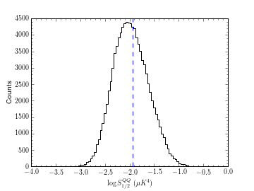
Figure 6: $S_{1/2}$ distribution for $C^{QQ}(\theta)$ with $r=0.1$. The blue dashed line shows the $\Lambda$CDM prediction for the ensemble average.

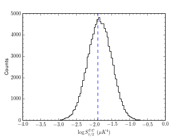
Figure 7: $S_{1/2}$ distribution for $C^{QQ}(\theta)$ with $r=0.1$. The blue dashed line shows the $\Lambda$CDM prediction for the ensemble average.

VI Conclusions

To address the lack of correlation in the temperature power spectrum at large angles in particular, we need to move beyond temperature data alone. We show two viable methods for calculating correlation functions on the sky that arise from polarization and presented the distributions for the corresponding statistics using constrained realizations for the E-mode contributions and the best-fit $\Lambda$CDM framework for B-mode realizations. A suppression in the primordial tensor or scalar fluctuations will affect the features of the two-point correlation function, meaning , local $C^{\hat{E}\hat{E}}(\theta)$ and $C^{\hat{B}\hat{B}}(\theta)$ as well as $C^{QQ}(\theta)$ and $C^{UU}(\theta)$, and their related statistical measures. This would lend considerable weight to the argument that the lack of correlation seen in $C^{TT}(\theta)$ is due to primordial physics, and is not just an anomalous statistical fluctuation of $\Lambda$CDM.

We presented the distribution for an $S_{1/2}$ statistic for a $C^{\hat{B}\hat{B}}(\theta)$ from $\Lambda$CDM cosmology with $r=0.1$. If future limits on the value of $r$ are found to be significantly below this value, the results for $C^{\hat{B}\hat{B}}(\theta)$ will scale appropriately, wheras results for all other correlation functions will remain unchanged. For $C^{\hat{E}\hat{E}}(\theta)$, $C^{QQ}(\theta)$, and $C^{UU}(\theta)$, we considered constrained realizations, where $a_{\ell m}^{E}$ coefficients were related to $a_{\ell m}^{T}$ coefficients that match our power spectrum measurements and give values of $S_{1/2}^{TT}$ at least as small as we observe on the full- and cut-sky. We showed that for a $\Lambda$CDM cosmology, the expected values of the statistics for Stokes parameter correlation functions are $S_{1/2}^{QQ}=0.0116\;\mu\mathrm{K}^{4}$ and $S_{1/2}^{UU}=0.0129\;\mu\mathrm{K}^{4}$, and the local E- and B-mode expected values are $S_{1/2}^{\hat{E}\hat{E}}=1.85\times 10^{5}\;\mu\mathrm{K}^{4}$ and $S_{1/2}^{\hat{B}\hat{B}}=218.3\;\mu\mathrm{K}^{4}$. We chose to keep the previously defined $S_{1/2}$ for analysis here, rather than generalizing to other angles than $\cos 60^{\circ}=1/2$, as the dominant secondary effect on polarization signals from epoch of reionzation is sufficiently close to the surface of last scattering to not change the relevant angle of suppression significantly. Late-time reionization contributes to the signal at a level 100 times smaller than the effect of reionization at $z=10$, so while those would skew the relevant angular scales, they are subdominant.

Using a polarization error estimates for Planck, PIXIE and PRISM outlined in Table 1, we calculated the resulting $S_{1/2}$ statistics from a sky with exact suppression above $60^{\circ}$. These values are presented in Table 2. We note that these levels are well below the $\Lambda$CDM predictions for all of the polarization correlation functions presented here, and pixel noise for future experiments will not be a significant source of error in identifying suppression. Measurement of large-angle polarization correlation functions will have errors dominated by systematics rather than map pixel noise for the foreseeable future.

Beyond being able to confirm that the suppression of temperature fluctuations is unlikely to be a statistical fluke, polarization correlation functions will add important new information. Because the local $\hat{E}$ and $\hat{B}$ correlation functions are dominated by large $\ell$ values, a suppression in all four correlation functions would strongly indicate that the suppression manifests itself physically in real-space at large angles. The $\hat{E}$ and $\hat{B}$ correlations give insight about suppression that is independent of any effects of reionization which dominate the $Q$ and $U$ correlations. Also, foreground emission will contribute differently to the various correlation functions.

Further, since the local $\hat{B}$ correlation is determined entirely by tensor fluctuations, a strong suppression in that correlation function and not in others would show that the primordial suppression is predominantly in the tensor perturbations, while suppressions in local $\hat{E}$, $Q$ and $U$ but not in local $\hat{B}$ would suggest that the scalar perturbations are suppressed.

The distribution for $S_{1/2}$ statistics for each constrained correlation function was compared to the distribution from $\Lambda$CDM alone. We found no significant difference between the two distributions and have presented only the constrained in this work. This means that polarization correlation functions provide a largely independent probe of correlations compared to the anomalous temperature correlation function. Future high-sensitivity measurements of polarization over large fractions of the sky from envisioned experiments like PIXIE Kogut:2011xw will differentiate primordial physics from a statistical fluke as the origin of this anomaly.

If the suppressed temperature correlation is due to a statistical fluke, then measurements of the polarization correlation function at large angular scales is likely to give a much less suppressed signal. If, on the other hand, the suppressed temperature correlation is due to some physical mechanism, how well can polarization test this scenario? The answer depends on the precise prediction of the suppression model. A Bayesian model comparison between a given model and the standard cosmology will give a quantitative answer to this question. We are currently investigating this possibility for a model with suppressed correlations in the primordial gravitational potential perturbations. In general, we expect suppressed primordial correlations will be evident in polarization at least as much as in temperature, due to the lack of an integrated Sachs-Wolfe contribution to the polarization perturbations. A strong discrimination between a suppressed-correlation cosmology and the standard cosmology is likely.

VII acknowledgements

The authors thank Sean Bryan, Ben Saliwanchik, and J.T. Sayre for useful conversations. AY is supported by NASA NESSF Fellowship. CJC, GDS and AY are supported by a grant from the US DOE to the Particle Astrophysics Theory group at CWRU. SA and AK are supported by NSF grant 1312380 through the Astrophysics Theory Program.

Appendix A Correlation Functions and $S(x)$ Calculations for $QQ$ and $UU$ in Terms of Wigner d Matrices

The $G^{\pm}_{\ell}(\cos\theta)$ functions described in II.2 can be expressed in terms of reduced Wigner matrices. This form may be useful for finding analytic expressions of $S_{1/2}^{QQ}$ and $S_{1/2}^{UU}$ which are easier to calculate numerically than performing the full integrals over $[C(\theta)]^{2}$. We can write the correlation functions for $Q$ and $U$ as

$$C^{QQ}(\theta)=\sum_{\ell}\frac{2\ell+1}{8\pi}\left(D_{\ell}^{+}(\cos\theta)C_{\ell}^{EE}+D_{\ell}^{-}(\cos\theta)C_{\ell}^{BB}\right)$$ (29)

and

$$C^{UU}(\theta)=\sum_{\ell}\frac{2\ell+1}{8\pi}\left(D_{\ell}^{-}(\cos\theta)C_{\ell}^{EE}+D_{\ell}^{+}(\cos\theta)C_{\ell}^{BB}\right)\;,$$ (30)

where we have assumed parity invariance and used

$$D^{\pm}_{\ell}(\cos\theta)\equiv\left[d_{2,2}^{\ell}(\theta)\pm d_{2,-2}^{\ell}(\theta)\right]$$ (31)

from Chon:2003gx , where $d_{i,j}^{\ell}(\theta)$ are the reduced Wigner rotation matrices.

This form of the correlation functions would lead to a method of calculating $S_{1/2}$ most similar to that defined in Copi:2013zja by using properties of d-matrix integrals and recursion relations.

The general form of the S statistic is defined as

$$S(x)\equiv\int_{-1}^{x}\left[C^{XX}(x)\right]^{2}\;\mathrm{d}x,$$ (32)

where $x=\cos\theta$ and $S_{1/2}=S(1/2)$. We define

$$I_{\ell\ell^{\prime}}^{\pm\pm}\equiv\int_{-1}^{x}d_{2,\pm 2}^{\ell}(x)d_{2,\pm 2}^{\ell^{\prime}}(x)\;\mathrm{d}x,$$ (33)

which we use to calculate $S(x)$ using properties of the reduced Wigner matrices.

Important properties of the $I_{\ell\ell^{\prime}}^{\pm\pm}$ matrices are that $I_{\ell\ell^{\prime}}^{+-}(x)=I_{\ell\ell^{\prime}}^{-+}(x)$ and

$$I_{\ell\ell^{\prime}}^{--}(x)=(-1)^{\ell+\ell^{\prime}}\left[\frac{2}{2\ell+1}\delta_{\ell\ell^{\prime}}-I_{\ell\ell^{\prime}}^{++}(-x)\right],$$ (34)

so all required quantities can be constructed from calculating $I_{\ell\ell^{\prime}}^{+-}(x)$ and $I_{\ell\ell^{\prime}}^{++}(x)$ only. To compute these, we use the relation betwen reduced Wigner matrices and the Clebsch-Gordan coefficients angmom , $C^{jm+m^{\prime}}_{\ell m\ell^{\prime}m^{\prime}}$:

$$d_{m_{1},m_{2}}^{\ell}(x)d_{m^{\prime}_{1},m^{\prime}_{2}}^{\ell^{\prime}}(x)=$$

$$\sum^{\ell+\ell^{\prime}}_{j=|\ell-\ell^{\prime}|}C^{jm_{1}+m_{1}^{\prime}}_{\ell m_{1}\ell^{\prime}m^{\prime}_{1}}C^{jm_{2}+m_{2}^{\prime}}_{\ell m_{2}\ell^{\prime}m^{\prime}_{2}}d^{j}_{m_{1}+m^{\prime}_{1}\;m_{2}+m^{\prime}_{2}}(x).$$ (35)

Combining Eq. (33) with Eq. (A) and exploiting properties of the Clebsch-Gordan coefficients, we find:

$$I_{\ell\ell^{\prime}}^{++}(x)=\sum^{\ell+\ell^{\prime}}_{j=\mathrm{max}(|\ell-\ell^{\prime}|,4)}\left[C_{\ell 2\ell^{\prime}2}^{j4}\right]^{2}\int_{-1}^{x}d_{44}^{j}(x)\;\mathrm{d}x$$ (36)

and

$$I_{\ell\ell^{\prime}}^{+-}(x)=\sum^{\ell+\ell^{\prime}}_{j=\mathrm{max}(|\ell-\ell^{\prime}|,4)}C_{\ell 2\ell^{\prime}2}^{j4}C_{\ell 2\ell^{\prime}-2}^{j0}\int_{-1}^{x}d_{40}^{j}(x)\;\mathrm{d}x.$$ (37)

The integrals have analytic solutions, which make computation of the $I_{\ell\ell^{\prime}}$ matrices more efficient. The integral over $d_{40}^{j}(x)$ is the simpler of the two cases:

$$i_{j}^{(0)}(x)\equiv\int_{-1}^{x}d_{40}^{j}(x)\,\mathrm{d}x.$$ (38)

This integral can be performed by noting that

$$d_{m0}^{j}(\beta)=\sqrt{\frac{4\pi}{2j+1}}Y_{jm}^{*}(\beta,0)=\sqrt{\frac{(j-m)!}{(j+m)!}}P_{j}^{m}(\cos\beta).$$ (39)

Using the Rodrigues formula,

$$P_{j}^{m}(x)=(-1)^{m}(1-x^{2})^{m/2}\frac{\mathrm{d}^{m}}{\mathrm{d}x^{m}}P_{j}(x),$$ (40)

and integrating by parts, we can show that

$$i_{j}^{(0)}(x) =\sqrt{\frac{(j-4)!}{(j+4)!}}\int_{-1}^{x}(1-x^{2})^{2}\frac{\mathrm{d}^{4}}{\mathrm{d}x^{4}}P_{j}(x)\,\mathrm{d}x$$

$$=\sqrt{\frac{(j-4)!}{(j+4)!}}\left(-\sqrt{1-x^{2}}P_{j}^{3}(x)\right.$$

$$+4xP_{j}^{2}(x)-4(1-3x^{2})\frac{\mathrm{d}P_{j}(x)}{\mathrm{d}x}$$

$$+4(-1)^{j}j(j+1)-24xP_{j}(x)-24(-1)^{j}$$

$$\left.+\frac{24}{2j+1}\left[P_{j+1}(x)-P_{j-1}(x)\right]\right).$$ (41)

The integral over $d_{44}^{j}(x)$ is more conveniently done as integrals over angles:

$$i_{j}^{(4)}(x)\equiv\int_{\cos^{-1}(x)}^{\pi}d_{44}^{j}(\beta)\sin\beta\,\mathrm{d}\beta.$$ (42)

Using the relation

$$\sin\beta\,d_{44}^{j}(\beta) =\frac{\sqrt{(j^{2}-4^{2})(j+3)(j+4)}}{j(2j+1)}d_{43}^{j-1}(\beta)$$

$$-\frac{4\sqrt{(j-3)(j+4)}}{j(j+1)}d_{43}^{j}(\beta)$$

$$-\frac{\sqrt{[(j+1)^{2}-4^{2}](j-3)(j+2)}}{(j+1)(2j+1)}d_{43}^{j+1}(\beta),$$ (43)

along with properties of integrals over $d_{43}^{j}(\beta)$, $d_{42}^{j}(\beta)$, $d_{41}^{j}(\beta)$, and $d_{40}^{j}(\beta)/\sin(\beta)$, the integral becomes

$$i_{j}^{(4)}(x) =\frac{\sqrt{(j^{2}-4^{2})(j+3)(j+4)}}{j(2j+1)}k_{j-1}(x)$$

$$-\frac{4\sqrt{(j-3)(j+4)}}{j(j+1)}k_{j}(x)$$

$$-\frac{\sqrt{[(j+1)^{2}-4^{2}](j-3)(j+2)}}{(j+1)(2j+1)}k_{j+1}(x),$$ (44)

where

$$k_{j}(x) =\sqrt{\frac{(j+2)(j-1)}{(j-2)(j+3)}}\ell_{j}(x)$$

$$\quad\quad+\frac{2}{\sqrt{(j-2)(j+3)}}d_{42}^{j}(x),$$ (45)

$$\ell_{j}(x) =\frac{1}{\sqrt{j(j+1)}}d_{40}^{j}(x)-\frac{4}{\sqrt{j(j+1)}}m_{j}(x),$$ (46)

and

$$m_{j}(x) =\sqrt{\frac{(j-4)!}{(j+4)!}}\left(-\frac{1}{\sqrt{1-x^{2}}}P_{j}^{3}(x)\right.$$

$$+\frac{2x}{1-x^{2}}P_{j}^{2}(x)+\frac{(-1)^{j}}{4}\frac{(j+2)!}{(j-2)!}$$

$$\left.-2\frac{\mathrm{d}}{\mathrm{d}x}P_{j}(x)-(-1)^{j}j(j+1)\right).$$ (47)

Recursion relations were used to calculate the Clebsch-Gordan coefficients from Eqs. (8.5:3), (8.5:8), and (8.6:27) in angmom .

We compute the $I_{\ell\ell^{{}^{\prime}}}^{(i)}$ matrices in Eq. (II.2) directly from these forms, as

$$I_{\ell\ell^{{}^{\prime}}}^{(1)}(x) = I_{\ell\ell^{\prime}}^{++}(x)+2I_{\ell\ell^{\prime}}^{+-}(x)+I_{\ell\ell^{\prime}}^{--}(x)$$

$$I_{\ell\ell^{{}^{\prime}}}^{(2)}(x) = I_{\ell\ell^{\prime}}^{++}(x)+I_{\ell\ell^{\prime}}^{--}(x)$$

$$I_{\ell\ell^{{}^{\prime}}}^{(3)}(x) = I_{\ell\ell^{\prime}}^{++}(x)-2I_{\ell\ell^{\prime}}^{+-}(x)+I_{\ell\ell^{\prime}}^{--}(x).$$ (48)

References

(1)
P. A. R. Ade et al. [Planck Collaboration],
arXiv:1303.5076 [astro-ph.CO].
(2)
R. Adam et al. [Planck Collaboration],
arXiv:1502.01582 [astro-ph.CO].
(3)
P. A. R. Ade et al. [Planck Collaboration],
arXiv:1502.01589 [astro-ph.CO].
(4)
P. A. R. Ade et al. [Planck Collaboration],
arXiv:1303.5083 [astro-ph.CO].
(5)
C. L. Bennett, A. Banday, K. M. Gorski, G. Hinshaw, P. Jackson, P. Keegstra, A. Kogut and G. F. Smoot et al.,
Astrophys. J. 464, L1 (1996)
[astro-ph/9601067].
(6)
D. N. Spergel et al. [WMAP Collaboration],
Astrophys. J. Suppl. 148, 175 (2003)
[astro-ph/0302209].
(7)
C. J. Copi, D. Huterer, D. J. Schwarz and G. D. Starkman,
Adv. Astron. 2010, 847541 (2010)
[arXiv:1004.5602 [astro-ph.CO]].
(8)
C. J. Copi, D. Huterer, D. J. Schwarz and G. D. Starkman,
Mon. Not. Roy. Astron. Soc. 399, 295 (2009)
[arXiv:0808.3767 [astro-ph]].
(9)
C. J. Copi, D. Huterer, D. J. Schwarz and G. D. Starkman,
arXiv:1303.4786 [astro-ph.CO].
(10)
A. Yoho, C. J. Copi, G. D. Starkman and A. Kosowsky,
arXiv:1310.7603 [astro-ph.CO].
(11)
M. Kamionkowski, A. Kosowsky and A. Stebbins,
Phys. Rev. D 55, 7368 (1997)
[astro-ph/9611125].
(12)
M. Kamionkowski, A. Kosowsky and A. Stebbins,
Phys. Rev. Lett. 78, 2058 (1997)
[astro-ph/9609132].
(13)
M. Zaldarriaga and U. Seljak,
Phys. Rev. D 55, 1830 (1997)
[astro-ph/9609170].
(14)
D. Baumann and M. Zaldarriaga,
JCAP 0906, 013 (2009)
[arXiv:0901.0958 [astro-ph.CO]].
(15)
L. Knox,
Phys. Rev. D 52, 4307 (1995)
[astro-ph/9504054].
(16)
P. A. R. Ade et al. [Planck Collaboration],
arXiv:1303.5062 [astro-ph.CO].
(17)
A. Kogut, D. J. Fixsen, D. T. Chuss, J. Dotson, E. Dwek, M. Halpern, G. F. Hinshaw and S. M. Meyer et al.,
JCAP 1107, 025 (2011)
[arXiv:1105.2044 [astro-ph.CO]].
(18)
P. Andre et al. [PRISM Collaboration],
arXiv:1306.2259 [astro-ph.CO].
(19)
G. Chon, A. Challinor, S. Prunet, E. Hivon and I. Szapudi,
Mon. Not. Roy. Astron. Soc. 350, 914 (2004)
[astro-ph/0303414].
(20)
Varshalovich, Dmitri Aleksandrovich and Moskalev, AN and Khersonskii, VK,
Quantum Theory of Angular Momentum,
1988,
World Scientific