Resonance Searches with an Updated Top Tagger

Abstract

The performance of top taggers, for example in resonance searches, can be significantly enhanced through an increased set of variables, with a special focus on final-state radiation. We study the production and the decay of a heavy gauge boson in the upcoming LHC run. For constant signal efficiency, the multivariate analysis achieves an increased background rejection by up to a factor 30 compared to our previous tagger. Based on this study and the documentation in the Appendix we release a new HEPTopTagger2 for the upcoming LHC run. It now includes an optimal choice of the size of the fat jet, N-subjettiness, and different modes of Qjets.

I Introduction

After the discovery of the Higgs boson, a keystone of the Standard Model, one main task for the upcoming LHC runs will be searches for physics beyond the Standard Model. Several open experimental and theoretical questions point to additional particles or structures at energies above the electroweak energy scale review . A very generic feature of many extensions of the Standard Model is the presence of additional heavy particles which preferentially decay to a pair of top quarks tt_resonances . One example for such a resonance could be a heavy neutral $Z^{\prime}$-gauge boson with a TeV-scale mass. Historically, such states were only searched for using semi-leptonically decaying top pairs. There, a kinematic reconstruction is based on an approximate reconstruction of the missing neutrino momentum through a $W$-mass or top mass condition. In the last LHC run this search channel was supplemented by resonance searches based on boosted, hadronically decaying top pairs. In the corresponding ATLAS analysis atlas the HEPTopTagger heptop1 ; heptop2 and the template tagger template each showed a similar reach, comparable with the semileptonic channel. This experimental success is based on rapid progress in the field of just substructure both experimentally and theoretically, which will gain even more momentum during the 13 TeV LHC run.

The field of top and Higgs tagging tagging_review started essentially as a Gedankenexperiment to illustrate recombination jet algorithms seymour . After some early attempts for example to tag hadronically decaying tops early it took off with the development of the BDRS Higgs tagger with its mass drop condition understanding and a filtering step targeting underlying event and pile-up bdrs . The first top taggers were simple, deterministic algorithms which could identify and reconstruct hadronically decaying top quarks including subjet $b$-tagging hopkins ; heptop1 ; soft_drop ; mass_jump . They were based on deliberately simple structures and algorithms, to firmly establish subjet methods in ATLAS and CMS. After the experimental success of these completely new analysis tools in the first run of the LHC, the upcoming run will benefit from more advanced top tagging methods. Those include multivariate taggers heptop4 , template taggers template , as well as shower deconstruction shower_deco or event deconstruction event_deco . For those specialized tools the challenge will be to still provide a universal top tagging approach, which on the one hand allows for optimal experimental results, but on the other hand identifies and reconstructs boosted top quarks independent of the specialized analysis framework.

Over time, the original HEPTopTagger heptop1 has gone through several rounds of improvements. The first modification included a re-formulation of the algorithm, leading to the trademark A-shaped kinematic cuts heptop2 . One of the key observations leading to these cuts is that in the absence of a $b$-tag it is not helpful to uniquely identify the two $W$-decay jets because in typical top decays there will be two jet-jet combinations which reconstruct to an invariant mass around $80~{}\text{GeV}$ no_tc . The first set of new, additional variables heptop3 then included a combination of the usual filtered top mass bdrs with a pruned top mass pruning . In this upgrade we introduce a fat jet radius up to $R=1.8$ for moderately boosted tops and allow for a choice of Cambridge–Aachen ca_algo and $k_{T}$ kt_algo ; fastjet jet algorithms in all internal clustering and filtering steps except for the mass drop condition. This improves the tagging performance for highly boosted tops heptop3 . Recently, the algorithm was slightly changed to avoid background shaping heptop4 . In the same study we added a low-$p_{T}$ mode based on Fox–Wolfram moments fwm to incorporate angular correlations, extending the tagging coverage to $p_{T,t}=150~{}\text{GeV}$.

In this paper we present a detailed study of the HEPTopTagger2, collecting all previous modifications, as well as a whole range of new features targeted at multivariate analyses and statistical approaches to single events qjets ; telescoping . The main body of the paper will focus on $Z^{\prime}$ searches, where final-state jet radiation turns out to be the limiting factor of the original tagger. After resolving the issue with final-state radiation we will step by step improve the tagging algorithm by defining and including additional kinematic information. Finally, we will compare the multivariate tagging performance with the leading projections based on event deconstruction event_deco .

The main background in fully hadronic $Z^{\prime}\to t\bar{t}$ searches is QCD multi-jets production, which allows us to directly translate all our findings into a performance study based on tagging $t\bar{t}$ pairs in the Standard Model. We will show these results together with a review of the complete HEPTopTagger2 algorithm and the code interface in the Appendix.

II Resonance reconstruction

The key challenge of any top tagger is its broad range of applications and the related optimization of the algorithms and codes. For example, the HEPTopTagger was developed to solve the combinatorial problems in $t\bar{t}H$ searches heptop1 . The first public tagging code was presented for supersymmetric top partner searches in semi-leptonic top decays heptop2 . Its proposed applications include single top production to experimentally separate the $s$-channel and $t$-channel production processes single_top . However, its experimental application during the first LHC run was the search for heavy resonances decaying to hadronic $t\bar{t}$ searches atlas . For such a resonance search the kinematic top tagger in combination with a $b$-tag showed a similar performance as the usual, approximate reconstruction of semileptonic $t\bar{t}$ pairs. In this paper we will present a set of improvements towards the HEPTopTagger2 for a $Z^{\prime}$ search at the 13 TeV LHC. Many of these improvements can be applied to other LHC processes, as will be discussed in the Appendix.

In using all available information from a pair of boosted top quarks, event deconstruction is currently giving the leading performance estimates for heavy resonance searches event_deco . For the analysis in the main body of this paper we will follow the analysis framework of Ref. event_deco , to eventually allow for a comparison in Sec. IV. For the signal we therefore use Pythia8 pythia to generate $Z^{\prime}\to t\bar{t}$ events with $m_{Z^{\prime}}=1500~{}\text{GeV}$ at 13 TeV collider energy. Assuming the same couplings as for the Standard Model $Z$-boson would yield a width of $\Gamma(Z^{\prime})=47~{}\text{GeV}$; to be consistent with the assumed experimental resolution in Ref. event_deco we increase the width to $65~{}\text{GeV}$ and only simulate the vector couplings. However, we will see that this choice of the physical $Z^{\prime}$ width does not affect our results which are based on the reconstructed fat jet kinematics. For the $Z^{\prime}$ decay we assume a 100% branching ratio to top pairs. The two backgrounds are continuum $t\bar{t}$ production which we simulate assuming $p_{T,t}>400~{}\text{GeV}$, and QCD di-jet production, also requiring $p_{T,j}>400~{}\text{GeV}$. Again, we rely on Pythia8, keeping in mind that for the pure QCD background our di-jet rate might not be a conservative estimate. All top quarks are forced to decay hadronically. Our simulations for the main body of the paper include underlying event but do not account for pile–up or detector effects, unless explicitly mentioned. For a completely realistic study of the signal and background efficiencies of the new HEPTopTagger2 we will have to rely on upcoming experimental studies. For our multivariate tagging analyses we optimize the background rejection with respect to the pure QCD background, because it is by far dominant.

Decay kinematics

On the analysis level we first select events with at least two fat jets with

$$p_{T,\text{fat}}>400~{}\text{GeV}\qquad\qquad\text{and}\qquad|y_{\text{fat}}|<2.5\;,$$ (1)

reconstructed using the C/A algorithm ca_algo with cone size $R=1.5$, as implemented in FastJet fastjet . We limit ourselves to the two hardest fat jets in each event for the $Z^{\prime}$ search. The corresponding cut flow is given in Tab. 1. Using the old default HEPTopTagger setup heptop2 we find a double top tagging efficiency of $\varepsilon_{\text{2tags}}=14\%$ in the signal, as shown in Tab. 1. If we apply a fixed invariant mass window $m_{tt}\in[1200,1600]~{}\text{GeV}$ on the tagged and reconstructed top quarks, the $Z^{\prime}$ tagging efficiency is $\varepsilon_{Z^{\prime}}=10.2\%$. For the $t\bar{t}$ background we find mis-tagging probabilities of $\varepsilon_{\text{2tags}}=13.7\%$ and $\varepsilon_{Z^{\prime}}=3.3\%$. For the QCD background sample the double mistag rates are $\varepsilon_{\text{2tags}}=6.6\cdot 10^{-4}$ and $\varepsilon_{Z^{\prime}}=1.5\cdot 10^{-4}$. The QCD jets background exceeds the continuum top pair production by a factor five after all cuts.

	$Z^{\prime}\to t\bar{t}$	$t\bar{t}$	QCD
generator level	$10^{5}$	$10^{5}$ (1.76 pb)	$8\cdot 10^{6}$ (1.93 nb)
$\geq$ 2 fat jets Eq.(1)	69142	85284 (1.50 pb)	$6.7\cdot 10^{6}$ (1.62 nb)
hardest 2 fat jets HTT[JHEP1010] tagged	9679	11706 (0.21 pb)	4426 (1.07 pb)
$m_{tt}\in[1200,1600]~{}\text{GeV}$	7031	2817 (0.05 pb)	978 (0.24 pb)

Table 1: Number of events and the corresponding Pythia8 cross section used for our analysis. The efficiencies $\varepsilon_{S,B}$ for a $Z^{\prime}$ extraction are defined as the ratio of the last to the second line in this table.

A straightforward improvement of the basic analysis shown in Tab. 1 should be to replace the mass window by a boosted decision tree (BDT) analysis, as implemented in Tmva tmva , based on the reconstructed invariant mass $m_{tt}$. In the left panel of Fig. 1 we first show the results as receiver operator characteristic (ROC) curve, correlating the best signal and background efficiencies based on a given set of kinematic observables. This approach has been used to improve and benchmark the general performance of the HEPTopTagger heptop4 . Because the QCD jet background is dominant we always set up our multivariate analyses based on the $Z^{\prime}$ signal and the QCD background sample. Compared to the working point of the original public HEPTopTagger tool heptop2 with a fixed mass window $m_{tt}\in[1200,1600]~{}\text{GeV}$ the new HEPTopTagger2 including $m_{tt}$ in a multivariate analysis looks slightly worse. The reason is the change in the order in the algorithm described in the Appendix. It significantly reduces the background sculpting, but at the expense of background rejection for example for a constant signal efficiency. On the other hand, the reduced background sculpting removes a major source of systematic uncertainty when we need to interpret an $m_{tt}$ distribution which shows a peak which could be due to a signal or to a sculpted background. Moreover, it turns out that the difference between the old and new taggers vanishes once both of them are used in a fully flexible multivariate framework.

Figure 1: Left: ROC curves for the dominant QCD background vs. the $Z^{\prime}$ signal after including additional kinematic information shown in Eq.(2). As in all figures the asterisk corresponds to the original HEPTopTagger described in Ref. heptop2 . Right: $|\Delta y|$ distribution of the reconstructed top quarks for signal and backgrounds.

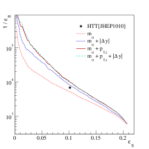
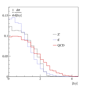
For a better discrimination between signal and background we should include additional variables in our multivariate analysis. The deterministic structure of the HEPTopTagger will still allow for a particularly clear separation of the actual tagging and reconstruction from a subsequent kinematic analysis based on the reconstructed top momenta. The first additional variable we include is the rapidity difference between the two reconstructed top quarks, $|\Delta y|$. The corresponding signal and background distributions are shown in the right panel of Fig. 1. While this variable might not be too efficient in removing the $t\bar{t}$ continuum background, events are visibly less central for QCD jets. The differences can hardly be translated into efficient kinematic cuts, but they will help as part of a multivariate analysis. In the left panel of Fig. 1 we show the corresponding improvement in terms of ROC curves. In particular for low signal efficiencies $\varepsilon_{S}<0.1$ we find a significant reduction of the background fake rates, going beyond the working point of the first HEPTopTagger.

An obvious extension of our set of kinematic observables are the transverse momenta of the reconstructed top quarks. Note that as part of the ROC analysis we do not have to ensure that the different kinematic variables are independent of each other, which would be problematic for a combination of $m_{tt}$ and the $p_{T,t}$ distributions. Again, the improvement from the transverse momentum spectra is shown in the left panel of Fig. 1. All this illustrates that the kinematic information on the tagged and reconstructed tops can increase the background rejection by 50% to 100% for fixed signal tagging efficiency. We also see that once we include the top–pair invariant mass and the transverse momenta, the additional improvement from $|\Delta y|$ vanishes, because the 2-particle final state is essentially fully described. As kinematic observables in our multivariate analysis we choose

$$\{\;m_{tt},p_{T,t_{1}},p_{T,t_{2}}\;\}\qquad\qquad\text{(decay kinematics).}$$ (2)

QCD jets

In purely hadronic searches for new physics, QCD effects beyond fixed order are a major issue in trying to theoretically understand the signal and backgrounds. Before we devise strategies to deal with final-state radiation and initial-state radiation in heavy-resonance searches we can estimate their effect on the naive tagger–based analysis.

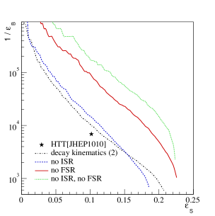
On the Monte Carlo level it is possible to separately remove initial-state radiation and final-state radiation from all signal events. For the QCD jets background this is not sensible, because we need both mechanisms to generate a sufficient jet multiplicity. The ROC curves in Fig. 2 show the expected improvements in the absence of additional signal jets. We see that the leading effect spoiling the signal extraction is final-state radiation (FSR). Initial-state radiation (ISR) affects top tagging in two ways. First, the additional QCD jets can mimic for example the softer $W$-decay jet and degrade the tagging efficiency through combinatorics. On the other hand, ISR jets recoil against the $Z^{\prime}$, affecting the $p_{T}$ spectrum of the top quarks. In particular the tagging of the softer top decay can benefit from this recoil, which means that for large signal efficiency the results without ISR become worse than those with all jet activity included.

As a whole, the results shown in Fig. 2 indicate potentially significant improvements of top taggers when we target the different effects of QCD jet radiation. We will show in the following subsection how a deterministic top tagger is limited by final-state radiation and how the new HEPTopTagger2 can avoid these issues. Combinatorial problems related to initial-state radiation will then be one of the key topics in Sec. III.

Figure 2: ROC curves for different combinations of initial-state jet radiation (ISR) and final-state jet radiation (FSR) in the $Z^{\prime}$ signal generation. The background is QCD with ISR and FSR for all curves.

Final-state radiation

Final-state radiation (FSR) turns one of the key advantages of our top tagger into a significant problem: unlike some other top tagging approaches, the HEPTopTagger returns the 4-momentum of the tagged top, including a cut on the reconstructed top mass $m_{\text{rec}}\in[150,200]~{}\text{GeV}$ heptop4 . This allows us to trivially reconstruct $m_{Z^{\prime}}$. Final-state radiation off the top decay products will be captured by the jet clustering and contribute to the correct filtered top mass value bdrs . This way it will not pose a problem as long as the $Z^{\prime}$ decays to on-shell tops.

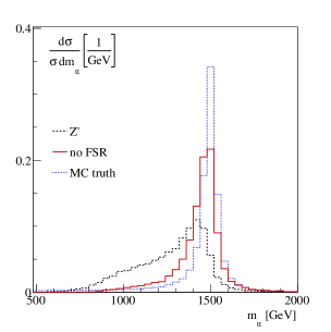
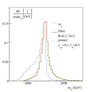
However, if the $Z^{\prime}$ decays to slightly off-shell tops, which turn themselves into on-shell tops, this final-state radiation off the intermediate top mis-aligns the actual $Z^{\prime}$ with the $Z^{\prime}$ as reconstructed from the top quarks at the moment they decay. Because the hard radiated gluon does not enter the top reconstruction, the top tag will pass, but lead to an underestimated $m_{Z^{\prime}}$ value. In the left panel of Fig. 3 we indeed see that the $m_{tt}$ distribution for the top-tagged signal correctly peaks around $m_{Z^{\prime}}$, but develops a sizeable asymmetric tail towards smaller $m_{tt}$ values. While the details of this asymmetric tail from Pythia8 should be subject to a detailed Monte Carlo study, we simply confirm that turning off final-state radiation by hand gets rid of it almost entirely. The remaining slight broadening as well as a minimal tail towards smaller $m_{tt}$ values is due to small losses in the top 4-momentum reconstruction of the tagger. At higher values of $m_{Z^{\prime}}$ the asymmetric tail is further enhanced.

Figure 3: Effect of final-state radiation on the invariant mass of the tagged and reconstructed $t\bar{t}$ system $m_{tt}$ for the $Z^{\prime}$ signal (left) and different approaches to reconstruct the $Z^{\prime}$ mass peak (right). Monte Carlo truth is $\sqrt{p_{Z^{\prime}}^{2}}$ with an assumed width of $65~{}\text{GeV}$.

The problem with large asymmetric tails from final-state radiation is that they cannot simply be corrected for in a universal top tagger. The basic structure of the HEPTopTagger has to identify and reconstruct top quarks, rather than the decay products of a heavy $Z^{\prime}$ resonance. Therefore, we do not modify the actual tagger, but we account for final-state radiation through an additional set of kinematic observables.

	$m_{\text{peak}}$ [GeV]	$\Gamma$ [GeV]	$\varepsilon^{\pm 150}_{Z^{\prime}}$	$1/\varepsilon^{\pm 150}_{tt}$	$1/\varepsilon^{\pm 150}_{\text{QCD}}$
$m_{tt}\in[1200,1600]~{}\text{GeV}$	–	–	0.136	22	2805
unfiltered	1539	167	0.141	21	1960
$R=0.3$, $N=4$	1457	152	0.146	28	2218
$R=0.3$, $N=5$	1477	144	0.150	25	2098
$R=0.3$, $N=6$	1489	139	0.151	25	2052
$R=0.3$, $N=7$	1496	144	0.151	24	2043
$R=0.2$, $N=5$	1443	140	0.141	29	2329
$R=0.3$, $N=5$	1477	144	0.150	25	2098
$R=0.4$, $N=5$	1500	144	0.151	24	2030
$R=0.5$, $N=5$	1515	143	0.148	23	1993
pruning $z=0.1$, $f_{R}=0.5$	1443	150	0.138	26	2075

Table 2: Breit–Wigner fits and performance of different grooming approaches. The quoted efficiencies are based on a window for the invariant mass of the two filtered fat jets $|m_{\text{ff}}-m_{Z^{\prime}}|<150~{}\text{GeV}$.

Following the brief discussion above, including the kinematics of the fat jet in addition to the reconstructed top 4-momentum should remove the broad asymmetric tail in the reconstructed $m_{Z^{\prime}}$ values. Again, we first select events with two tagged tops, including the top mass condition. Instead of using the 4-momenta of the tagged tops, we now reconstruct the $Z^{\prime}$ mass from the 4-momenta of the two fat jets of size $R=1.5$, which eventually lead to the top tags. In the presence of underlying event and initial-state radiation the naive $m_{\text{ff}}$ distribution peaks roughly at the correct $Z^{\prime}$ mass and shows symmetric tails. To use the invariant mass of the two fat jets we need to apply filtering bdrs . In the right panel of Fig. 3 we compare the filtered invariant mass from the two fat jets bdrs and its pruned value pruning , both as implemented in FastJet fastjet . As a reference we also show the $m_{tt}$ distribution from the left panel of the same figure. Unlike the reconstructed $m_{tt}$ distribution, both, the filtered and the pruned $m_{\text{ff}}$ distributions give symmetric peaks around the correct $m_{Z^{\prime}}$ value.

To be able to use the filtered $m_{\text{ff}}$ values in our HEPTopTagger analysis we confirm that filtering and pruning give stable numerical results for the invariant mass of the two fat jets. Results for different parameter settings are listed in Tab. 2. We give the peak positions, which would be subject to a proper calibration, the fitted Breit–Wigner widths for the symmetric peaks, and the tagging performances for a fixed mass window $|m_{\text{ff}}-m_{Z^{\prime}}|<150~{}\text{GeV}$. Replacing the Breit–Wigner width with a Gaussian would make no difference, but give a poorer modelling of the tails. Typical widths of the reconstructed $Z^{\prime}$ mass peak will range around $145~{}\text{GeV}$, roughly twice the assumed particle width of $65~{}\text{GeV}$. Even in the absence of detector effects, this resolution will replace the assumed particle width of $65~{}\text{GeV}$ in all of the following analysis. The constant numbers in Tab. 2 confirm that the $m_{\text{ff}}$ criterion is stable for different filtering parameters as well as pruning.

On the other hand, the results shown in Tab. 2 also indicate that simply replacing the $m_{tt}$ window by a filtered $m_{\text{ff}}$ value will not improve the $Z^{\prime}$ extraction. In Fig. 4 we show that the steeply falling QCD jets background now has a maximum around $m_{\text{ff}}=1.3~{}\text{TeV}$, while for the reconstructed top quarks there exists a much more pronounced maximum around $m_{tt}=900~{}\text{GeV}$. The reason is that top tagging removes events with many hard QCD jets in two steps: first requiring the correct top mass value from three assumed top decay products, and second when applying the $Z^{\prime}$ mass window. If we remove the first step, the second one has to deal with larger backgrounds at high $m_{\text{ff}}$ values.

Figure 4: Reconstructed mass distribution of the $Z^{\prime}$ signal and the backgrounds based on the tagged tops (left) and the corresponding filtered fat jets (right).

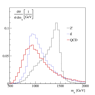
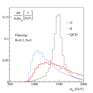
If we want to include final-state radiation and at the same time benefit from its additional information, we need to keep $m_{\text{ff}}$ as well as $m_{tt}$ in our analysis, and not apply a simple mass window on the $m_{tt}$ distribution. The kinematics of the $Z^{\prime}$-decay is then described by

$$\{\;m_{tt},m_{\text{ff}},p_{T,t_{1}},p_{T,t_{2}},p_{T,\text{f}_{1}},p_{T,\text{f}_{2}}\;\}\qquad\qquad\text{(filtered fat jets).}$$ (3)

All default settings of the HEPTopTagger are listed in the Appendix. We filter the fat jets using $R=0.3$ and keep the $N=5$ hardest substructures. In the left panel of Fig. 5 we show the corresponding ROC curves. Unlike in the rest of the paper we study the $t\bar{t}$ and QCD jets backgrounds separately. The improvement of the full multivariate tagger including the fat jet information of Eq.(3) is obvious for both backgrounds. In the right panel of Fig. 5 we first show the same improvement, but using a BDT trained on the QCD jets background only. Compared to the original HEPTopTagger we achieve an improvement of up to a factor 2 in $1/\varepsilon_{B}$ for constant signal efficiency. We note that for the QCD background the combination of mis-tagged top kinematics and fat jet kinematics goes beyond the description of the hard process. For example initial-state radiation, sensitive to the color structure of the signal and the background, will be captured in this combination of observables. On the other hand, because the fat jets are defined using the standard jet algorithms and show a stable filtering performance, we do not envision major experimental problems provided pile-up subtraction works as well as expected.

Figure 5: Left: performance of the multivariate analysis including the information on the fat jet, as given in Eq.(2), Eq.(3) and Eq.(4). Only in this plot do we optimize for $t\bar{t}$ and QCD backgrounds separately. Right: performance curve for the full analysis only accounting for the dominant QCD jet background.

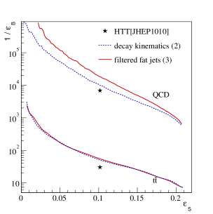
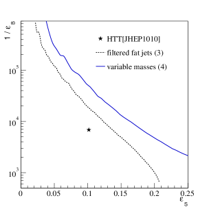
The set of kinematic observables listed in Eq.(3) still relies on the deterministic HEPToptagger output. This means that the identification of a $Z^{\prime}$ signal event is limited by the efficiency of two top tags. The choice of a working point in the top tagging algorithm will therefore limit our over-all efficiency. On the other hand, we already know that for hadronic $Z^{\prime}$ searches the QCD jets background is dominant and will only be reduced through a combination of top tags and $Z^{\prime}$ mass reconstruction.

In addition, we omit a fixed mass window for the reconstructed top mass $m_{\text{rec}}$. Instead, we widely open the top mass and $W$-mass constraints in the tagging algorithm. For each of the tops the corresponding $m_{\text{rec}}$ value then becomes an output of the tagger. We provide the multivariate $Z^{\prime}$ analysis with the smaller and larger of these two output $m_{\text{rec}}$ values, which we label as $m_{\text{rec}}^{\text{min}}$ and $m_{\text{rec}}^{\text{max}}$ respectively. Similarly, we avoid a fixed window for the ratio of the $W$-mass to the top mass, parametrized as $f_{W}$ in the tagging algorithm. Its deviation from the true value is given by the value of $f_{\text{rec}}$ defined in the Appendix. In the multivariate analysis we include the maximum of the two $f_{\text{rec}}$ values corresponding to each tagged top.

$$\{\;m_{tt},m_{\text{ff}},p_{T,t_{1}},p_{T,t_{2}},p_{T,\text{f}_{1}},p_{T,\text{f}_{2}},m_{\text{rec}}^{\text{min}},m_{\text{rec}}^{\text{max}},f_{\text{rec}}^{\text{max}}\;\}\qquad\qquad\text{(variable masses).}$$ (4)

The result is shown in the right panel of Fig. 5, where the range of accessible efficiencies eventually extends to $56\%$. Altogether, the analysis based on the set of kinematic variables shown in Eq.(4) gives us an improvement of up to a factor 5 in background rejection for a constant $Z^{\prime}$-signal efficiency.

III Updated tagger

Fat jets with a geometric size of $R=1.5$ or even $R=1.8$ have shown to be powerful new analysis objects at the LHC. The radius of the fat jet is directly related to the energy or boost of the heavy particles which can be captured. This means that a multi-purpose top tagger will be based on as large fat jets as possible. However, to realize their potential such large jets require additional treatment linked to their large geometric size. Without a dedicated analysis step, underlying event and pile-up will almost entirely wash out any structure inside the fat jet. Filtering bdrs as an integral part of all versions of the HEPTopTagger heptop1 ; heptop2 effectively reduces the geometric size of the fat jet used to reconstruct the top 4-momentum by introducing a second clustering stage with higher resolution. This solves the problem with underlying event and pile-up, but there remains a combinatorial problem caused for example by initial-state radiation. In particular the softer of the two subjets from the $W$-decay can easily be faked by a typical QCD jet inside the fat jet. This will lead to a wrong reconstruction of the top 4-momentum, which we can only counter by applying harder tagging requirements and hence reducing the tagging efficiency. These so-called type-2 tags heptop3 , where only two of three top decay jets can be identified with a parton-level decay quark have been in the focus of HEPTopTagger studies at moderate boost heptop3 ; heptop4 ; moderate . In the reconstruction of heavy resonances we can solve the problem of (too) large fat jets by adapting the size of the fat jet to the kinematics of the tagged top. It turns out that this adaptive size of the fat jet also gives us another powerful kinematic variable for the multivariate analysis. Finally, we will show how this optimalR modification of our tagging algorithm can be further improved by including $N$-subjettiness variables.

OptimalR mode

There have been different attempts to adjust the size of the fat jet for example based on the transverse momentum of the fat jet hopkins ; telescoping ; variableR , but none them lead to a dramatic effect in the performance of taggers. We instead choose a purely algorithmic way of determining the minimum size of the fat jet strebler . Assuming that three top decay jets are captured by the fat jet we can run the standard HEPToptagger algorithm to determine the top mass from the three leading subjets heptop4 . For a large fat jet size, typically $R=1.5$ or $R=1.8$, we compute a reference value of $m_{\text{rec}}$, which should be around the top mass. In the usual tagging algorithm, this computation of $m_{\text{rec}}$ from filtered subjets takes into account final-state radiation off the on-shell top. We then reduce the size of the fat jet in steps of $\Delta R=0.1$ and compute the corresponding values of $m_{\text{rec}}(R)$. In case of several possible triplets, this includes the step of choosing the one closest to the physical top mass, as described in step (5) in the Appendix. As a function of the decreasing jet size $R$ the fat jet mass $m_{\text{rec}}(R)$ will form a stable plateau, until the reduced fat jet will be too small to capture all three top decay jets. At this point $m_{\text{rec}}(R)$ will leave the plateau and show a significant drop. For $R=1.5$, which is sufficient for the $Z^{\prime}$ mass in our study, we define this drop through

$$\frac{m_{\text{rec}}^{(1.5)}-m_{\text{rec}}(R)}{m_{\text{rec}}^{(1.5)}}>0.2\qquad\Leftrightarrow\qquad R<R_{\text{opt}}\,.$$ (5)

Once the shrinking fat jet passes this condition we go back one step to the last $R$ value on the plateau and define this value as $R_{\text{opt}}$. The smallest value we allow in this study is $R_{\text{opt}}=0.5$, but for $p_{T,t}\gtrsim 1$ TeV this value can be adjusted in the tagger setup. This value could be a challenge of the calorimeter resolution, so the corresponding results are subject to tests based on a full detector simulation in ATLAS and in CMS. In this paper we typically arrive around $R_{\text{opt}}=0.6$. The tagging result for this $R_{\text{opt}}$ value will be the output of the top tagger.

Measuring $R_{\text{opt}}$ defines another useful variable for the top tagger, because we can also predict $R_{\text{opt}}$ from the fat jet kinematics. A similar reasoning is used in the original HEPTopTagger algorithm, where a consistency condition on the reconstructed top momentum $p_{T,t}>200~{}\text{GeV}$ ensures that the reconstructed top can actually be captured in the fat jet. In the optimalR mode we first determine the transverse momentum of the filtered fat jet, $p_{T,\text{f}}$ as described in the previous section. Including up to ten hardest subjets after a filtering step with $R_{\text{filt}}=0.2$ turns out to give the best estimate of $p_{T,\text{f}}$ for this purpose. Reducing this number to five subjets has no measurable effect on the width of the reconstructed $p_{T,\text{f}}$ distribution, but slightly shifts its maximum to smaller values strebler . The final number will be subject to an independent optimization in ATLAS and CMS.

For $p_{T,\text{f}}>200~{}\text{GeV}$ we derive a closed form by fitting a function $R_{\text{opt}}^{\text{(calc)}}\propto 1/p_{T,\text{f}}$ to simulated data, as described in the Appendix. The kinematic variables in our the multivariate tagger now read

$$\{\;m_{tt},m_{\text{ff}},p_{T,t_{1}},p_{T,t_{2}},p_{T,\text{f}_{1}},p_{T,\text{f}_{2}},m_{\text{rec}}^{\text{min}},m_{\text{rec}}^{\text{max}},f_{\text{rec}}^{\text{max}},R_{\text{opt}}-R_{\text{opt}}^{\text{(calc)}}\;\}\qquad\qquad\text{(optimalR).}$$ (6)

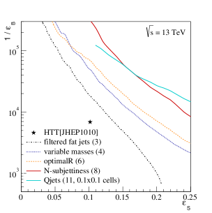
For this case of two top tags we choose $R_{\text{opt}}-R_{\text{opt}}^{\text{(calc)}}$ as the maximum deviation of the tagged tops. In this form all subsequent kinematic variables linked to the top tags will be evaluated with the fat jet size $R_{\text{opt}}$. For the $Z^{\prime}$ search $R_{\text{opt}}^{\text{(calc)}}$ will be strongly correlated with other kinematic variables listed in Eq.(6). We nevertheless include it in the BDT because the general multivariate HEPTopTagger2 described in the Appendix will not include the top momenta in the tagging. The increase of the tagging performance from the optimalR mode is shown in the left panel of Fig. 6. While for small signal efficiencies the curves for optimalR and for the variable mass setup of Eq.(4) are identical within numerical fluctuations, we observe a significant improvement for larger signal efficiencies.

Figure 6: Performance of the optimalR mode based on the kinematic variables in Eq.(6), including $N$-subjettiness variables as defined in Eq.(8), and including Qjets. As described in the text, for Qjets we need to require a finite calorimeter resolution, while all other curves do not include any detector effects. We only consider the dominant QCD background.

N-subjettiness

The arguably simplest question we can ask as part of a top tagger is the number of hard subjets inside the fat jet with a given jet mass. This number of subjets can be defined through an observable similar to event shapes like for example thrust, called $N$-subjettiness nsubjettiness ; better_obs . It is based on $N$ reference axes which are required to match the $k$ hard substructures,

$$\tau_{N}=\frac{1}{R_{0}\sum_{k}p_{T,k}}\sum_{k}p_{T,k}\min\left(\Delta R_{1,k},\Delta R_{2,k},\cdots,\Delta R_{N,k}\right)\;,$$ (7)

where $\Delta R_{i,j}$ is the geometric separation between the axis $i$ and the substructure $k$. In this form $N$-subjettiness parametrizes the deviation of the energy flow away from $N$ jets not only related to an integer number of subjets, but also reflecting the color structure and the related radiation pattern.

In terms of original definition nsubjettiness we fix the exponent to $\beta=1$. $R_{0}$ is an intrinsic cone size, chosen such that $\tau_{N}<1$. Small values of $\tau_{N}\to 0$ indicate that the complete substructure is described by $N$ axes, indicating that there are at most $N$ relevant substructures. The ratio $\tau_{N}/\tau_{N-1}$ will therefore become small for a fat jet with $N$ hard subjets. For top tagging the ratio $\tau_{3}/\tau_{2}$ will be most useful and can even be used as a tagger itself. Higher $\tau_{N}$ values will contribute to a multivariate analysis of $N$-subjettiness, describing the jet radiation pattern around the assumed three partonic top decay momenta.

We will use $N$-subjettiness as an additional variable in our multivariate HEPTopTagger. Originally, this combination did not lead to a significant improvement when added to the A-shaped cuts heptop4 . However, when we open the cut $f_{W}$ on the reconstructed ratio $m_{W}/m_{t}$ we observe a significant improvement for the extended set of kinematic variables. The complete set of relevant kinematic variables, now including $N$-subjettiness variables before and after filtering, is

$$\{\;m_{tt},m_{\text{ff}},p_{T,t_{1}},p_{T,t_{2}},p_{T,\text{f}_{1}},p_{T,\text{f}_{2}},m_{\text{rec}}^{\text{min}},m_{\text{rec}}^{\text{max}},f_{\text{rec}}^{\text{max}},R_{\text{opt}}-R_{\text{opt}}^{\text{(calc)}},\tau_{1,N},\tau_{1,N}^{\text{(filt)}},\tau_{2,N},\tau_{2,N}^{\text{(filt)}}\;\}\quad\text{($N$-subjettiness).}$$ (8)

For more details on the $N$-subjettiness variables we refer to the Appendix. As in Eq.(6) all kinematic variables linked to the top tag will be evaluated with the fat jet size $R_{\text{opt}}$. The details of implementation of the $N$-subjettiness variables is discussed in the Appendix.

Qjets

The main limitation even of the deterministic multivariate HEPTopTagger is the aim to identify a unique set of subjets from the top decay as part of the tagging procedure, which allows us to reconstruct the 4-momentum of the tagger top and for example compare it to Monte Carlo truth. If the kinematic selection identifies a wrong set of subjets as the best candidates for the top decay products, an actual top decay can easily fail the tagging procedure. To avoid this loss in signal efficiency we can allow for more than one set of candidate subjets to be tested. One approach that not only covers several candidates of subjet combinations, but which even allows for a statistical analysis of many such assignments is Qjets qjets .

During the clustering of the fat jet the standard recombination algorithms combine the closest set of pre-jets according to a given measure. For the C/A algorithm this measure is the geometric separation $d_{ij}=\Delta R_{ij}^{2}$ of the pre-jets $i$ and $j$. Qjets generalizes this deterministic choice to a likelihood measure. For each pair of pre-jets ($i,j$) it computes the weight

$$\omega_{ij}^{(\alpha)} =\exp\left(-\alpha\;\frac{d_{ij}-d_{ij}^{\text{min}}}{d_{ij}^{\text{min}}}\right)\;,$$ (9)

and then chooses the two pre-jets to cluster according to a random number trailing the weights $\omega_{ij}^{(\alpha)}$. For this study we choose $\alpha=0.1$, to balance the convergence of the algorithm with our aim of generating alternative subjet assignments for the top tagger. The standard jet algorithm corresponds to the limit $\alpha\to\infty$. The global weight for a clustering history is defined as

$$\Omega^{(\alpha)} =\prod_{\text{mergings}}\omega_{ij}^{(\alpha)}=\left[\prod_{\text{mergings}}\exp\left(-\frac{d_{ij}-d_{ij}^{\text{min}}}{d_{ij}^{\text{min}}}\right)\right]^{\alpha}\stackrel{{\scriptstyle\text{consistent}}}{{\longrightarrow}}1\;.$$ (10)

The universal limiting case $\Omega^{(\alpha)}\to 1$ for a perfect clustering history indicates that in searching for the largest global weight $\Omega$ the choice of $\alpha$ should not make a major difference. The Qjets clustering procedure can be repeated many times, where in this study we typically rely on 100 clustering histories. They can be ranked by their global weights $\Omega^{(\alpha)}$ instead of the independent local weights used by a deterministic jet algorithm. For each history we apply the unclustering and top tagging algorithm. As long as the deterministic jet algorithm picks a reasonable merging history for a signal event we expect the outcome of the deterministic tagger and the tagger acting on the clustering history with the highest global weight to be close.

The first advantage of Qjets appears when during an early clustering step the deterministic measure $d_{ij}$ identifies the wrong merging in the sense that the remaining history cannot be described well by QCD. This deterministic history will by definition receive the maximum global weight $\Omega^{(\alpha)}=1$. However, an alternative history in better agreement with QCD could reach a similarly large global weight. Because Qjets provides many alternative clustering histories, we can search for a set of top tags with comparably large global weights. For example, we can use the two positively tagged Qjets histories with the highest global weight in the multivariate analysis. This way, a possibly misleading deterministic result is corrected. This should improve the performance in particular when we enforce high signal efficiencies, where the tagger becomes most vulnerable to a wrong clustering input. It turns out that already this simple modification gives a sizeable improvement in the signal efficiency.

The second improvement to the usual top tagger is based on HEPTopTagger output for the full set of 100 clustering histories. First, we include the fraction of positive top tags based on the default HEPTopTagger settings among all 100 Qjets histories, $\varepsilon_{\text{Qjets}}$, as introduced in the Appendix. Next, we extract statistical information from distributions of the Qjets histories, like for example the reconstructed top mass $m_{\text{rec}}$. This distribution is defined for $\varepsilon_{\text{Qjets}}\times 100$ histories. Signal events will strongly peak around the top mass with a possible secondary peak around the $W$-mass. QCD background events will instead show a smooth decrease. The two most relevant observables in the $m_{\text{rec}}$ distribution are the mean and the variance of this reconstructed top mass distribution with 100 entries, symbolically denoted as $\{m_{\text{rec}}^{\text{Qjets}}\}$.

Our multivariate analysis we base on the second approach. We start with the top-tagged Qjets history with the highest global weight and run the tagging algorithm of this history only. In addition, we include the statistical information of the $m_{\text{rec}}$ distribution of the subset of the 100 Qjets histories which defines a top candidate. The complete list of observables including the Qjets information now reads

$$\{\;m_{tt},m_{\text{ff}},p_{T,t_{1}},p_{T,t_{2}},p_{T,\text{f}_{1}},p_{T,\text{f}_{2}},m_{\text{rec}}^{\text{min}},m_{\text{rec}}^{\text{max}},f_{\text{rec}}^{\text{max}},R_{\text{opt}}-R_{\text{opt}}^{\text{(calc)}},\{\tau_{N}\},\varepsilon_{\text{Qjets}}^{\text{min}},\{m_{\text{rec}}^{\text{Qjets}}\}\;\}\qquad\text{({Qjets}),}$$ (11)

where $\{\tau_{N}\}$ represents the appropriate set of filtered and unfiltered $N$-subjettiness variables (for example $N=1,2,3$ for each of the two tops). For the two tags in the $Z^{\prime}$ analysis we choose the smaller $\varepsilon_{\text{Qjets}}$ value of the two. All variables from the tagger are evaluated for the optimized $R$ size and the clustering history with the largest global weight.

In Fig. 6 we show the effect of the Qjets histories in addition to the other improvements. A key difference between the previous discussion and the Qjets approach is that we now need to include some kind of detector resolution, to limit Qjets to a manageable number of significantly different merging histories. For that reason we divide the calorimeter into $\eta\times\phi$ cells of size $0.1\times 0.1$ and pre-cluster the entire set of calorimeter entries before applying any jet algorithm. Because this detector resolution effect is not included for the previous results, the Qjets ROC curve does not consistently exceed the $N$-subjettiness curve without Qjets. On the other hand, we still observe the expected improvement towards large signal efficiencies. The moderate drop at small signal efficiencies gives us confidence that a full detector simulation will not lead to significant degradation of our results.

IV Full event information

Going back to the discussion in Sec. II the remaining question is how the new HEPTopTagger2 performance compares to other approaches designed for the upcoming LHC run. The benchmark for such a comparison is event deconstruction, or more specifically the projections for a $Z^{\prime}$ resonance search event_deco . As mentioned in our discussion of jet radiation in Sec.II the borders between the hard process or the $Z^{\prime}$ decay on the one side and QCD jet radiation and its sensitivity to the signal and background color structure on the other side are washed out when we include for example filtered subjets or $N$-subjettiness information. We therefore start with a brief discussion of the additional information from jets in the entire event and then move on to the comparison with the leading benchmark in proposed $Z^{\prime}$ analyses.

Additional jets

To determine to what degree the jet structure of purely hadronic $Z^{\prime}\to t\bar{t}$ events helps the extraction of the signal from the $t\bar{t}$ and QCD jets background we first study the number and kinematic distribution of small C/A jets with $R=0.2$ and $p_{T,j}>10~{}\text{GeV}$ in addition to the fat jets fulfilling Eq.(1). We choose these very small jets in order to test information which might be available from so-called microjets in shower deconstruction. Our discussion should not be applied to an LHC analysis one-to-one and is instead aimed at capturing as much information as possible. Without any major cuts, the number of jets will consist of three decay jets per top quark, FSR jets, and ISR jets. For an inclusive event sample, we should be able to tell apart the different processes from the number of jets and the kinematics of the individual jets scaling .

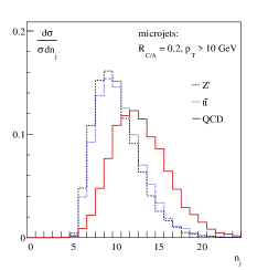
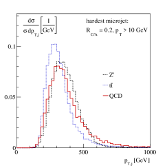
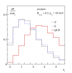
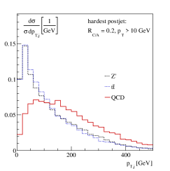
After a first level of cuts we see in Fig. 7 that the $Z^{\prime}$ signal and the $t\bar{t}$ background both peak at 10 microjets, e.g. four jets from ISR and FSR combined. For the background the number is slightly larger, because we generate the scale of the hard process also through a large number of jets. We also see that the transverse momentum of the hardest jet is slightly larger for the signal. We could include these jet patterns in a multivariate analysis, but at this stage this information would be very heavily correlated with the variables from the top tagger.

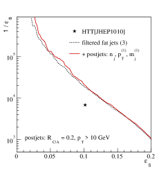
In a second step we focus on the jet activity which does not contribute to the top tagging. Inside the fat jets we know that the top tagger includes information based on subjets with typically $R=0.3$ and $p_{T}\gtrsim 20~{}\text{GeV}$ after filtering. After two tags we then remove all calorimeter data associated with the filtered triplet of either of the top candidates and re-cluster the remnants into microjets with $R=0.2$ and $p_{T,j}>10~{}\text{GeV}$. In the lower panels of Fig. 7 we see how after removing the signal decay jets the remaining number of jets peaks around two ISR or FSR jets. For the QCD background this number is higher, because it takes a larger number of equally distributed jets in the detector to fake a boosted massive top inside each fat jet. The transverse momentum of the hardest of the remaining QCD jets also peaks at very small values for the signal and the $t\bar{t}$ background, as one would expect for example for a small number of ISR jets. The bulk of the hardest QCD jets per event shows transverse momenta around $p_{T,j}=50-200~{}\text{GeV}$, still small compared to the hard scale imprinted on the multi-jet background through the kinematic selection of Eq.(1). We should be able to use this additional information for our BDT analysis, to improve the signal extraction. In the right panel of Fig. 7 we see the corresponding ROC curve. It turns out that almost all of the information available through the extra jet radiation is already included in our combined analysis of top tags and subjet kinematics.

Based on this piece of information we assume that additional jet information inside and outside the fat jets hardly changes the stable results of the updated top tagger, so we can compare the new HEPTopTagger2 to other multivariate methods.

Figure 7: Information on the hardest jet before top tagging (upper row) and the hardest jet left over after top tagging (lower row). For the jets defined with $R=0.2$ and $p_{T}>10~{}\text{GeV}$ we show the number of jets, the hardest jet’s transverse momentum, and its mass in $Z^{\prime}$ candidate events (left to right).

Comparison with other approaches

The most promising projections for boosted top identification and specifically searches for $t\bar{t}$ resonances during the upcoming LHC runs are available for shower deconstruction shower_deco or event deconstruction event_deco . This method is based on a construction of likelihoods representing possible shower histories for a jet or a fat jet. The underlying objects are so-called C/A ca_algo ; fastjet microjets with $R=0.2$ and $p_{T}>10~{}\text{GeV}$ event_deco . They are slightly softer and smaller than the subjets in a typical top tagger, but we have seen that the additional information from those jets should not make a big difference. Unlike general template methods, shower deconstruction relies on the soft and/or collinear approximation of QCD to compute the likelihood of a given shower history in terms of splitting probabilities and Sudakov factors (non-splitting probabilities). Based on the possible shower histories the likelihood ratio of a fat jet coming from a boosted top quark or from the QCD jet background acts as a measure for the top tag. One problem with shower deconstruction, like any probabilistic approach, is that we cannot separate the identification and the reconstruction of the boosted top quark. This means we cannot for example show the quality of the reconstructed 4-momentum compared to Monte Carlo truth.

The $Z^{\prime}$ analysis using event deconstruction starts with two fat jets of size $R=1.5$ and the acceptance cuts given in Eq.(1). The number of microjets is limited to 9 per fat jet. In addition to the likelihood separating the top or QCD origin of each of the two fat jets, the event likelihood measure now also includes a likelihood describing the resonant or non-resonant production of the pair of fat jets given their 4-momenta. At the level of the hard process this part is not very different from the established matrix element method me_method and largely replaces an analysis of the $m_{tt}$ and $p_{T,t}$ distributions defining the multivariate analysis of Eq.(2). In Ref. event_deco the observable width of the $m_{tt}$ resonance is assumed to range around $65~{}\text{GeV}$, an assumption we follow. In our analysis the precise resolution for example after detector effects only plays a secondary role, because the resolution of the HEPTopTagger2 is limited to $145~{}\text{GeV}$, as shown in Tab.2.

Figure 8: Comparison of the multivariate HEPTopTagger2 analysis presented in this paper with the event deconstruction approach of Ref. event_deco . All HEPTopTagger2 curves correspond to Fig. 6, but now with a collider energy of 14 TeV instead of 13 TeV, This comparison in the absence of an experimental validation should be taken as first estimate.

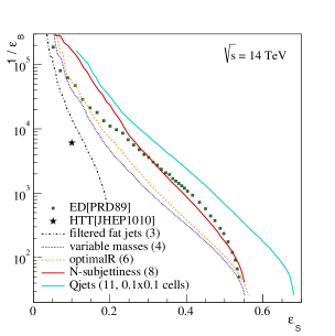
In Fig. 8 we show the performance of the analysis developed in this paper with the recent benchmark of event deconstruction. One difference to the HEPTopTagger results shown in Fig. 6 is that we now show $Z^{\prime}$ efficiencies up to 68%, confirming that Qjets indeed gives us a major improvement for very large signal efficiencies. Another difference is that for a direct comparison we now assume a collider energy of 14 TeV. Both, event deconstruction and the new HEPTopTagger show a comparable performance for the upcoming run. The final answer on both methods will only be given by experimental studies including data.

V Conclusion

We demonstrated how the updated HEPTopTagger2 performs in searches for $Z^{\prime}$ bosons or other heavy resonances decaying to top pairs in the upcoming LHC run. Based on the original HEPTopTagger heptop2 we modify the tagging algorithm and add several additional kinematic variables to a multivariate analysis:

• fat jet kinematics to account for final-state radiation in resonance searches;

• algorithmically optimized size of the original fat jet combined with its prediction (optimalR mode);

• $N$-subjettiness probing the more general subjet structures inside the fat jet;

• Qjets with a global picture of the most likely clustering histories giving a top tag.

Each of these improvements can be added to the top tagging individually. For the specific $Z^{\prime}$ resonance search we altogether achieve an increase of the background rejection by a factor of $30$ for a constant $Z^{\prime}$-signal efficiency of $10\%$. Compared to the original tagger heptop2 the background sculpting in the invariant mass of the top pair is significantly reduced heptop4 . These updated results are at least competitive with the leading estimates for other tagging methods.

Because the multivariate $Z^{\prime}$ analysis includes several layers of improvement, not necessarily linked to the actual top tagging, we also show in the Appendix the corresponding improvements for top tagging in $t\bar{t}$ events. There, we test the updated tagger for moderate ($p_{T,t}>200$ GeV) and sizeable ($p_{T,t}>600$ GeV) boost and find a significant improvement in particular for larger boost. The limiting factor for moderate boost still is capturing all three top decay jets inside a fat jet, which has to be targeted by a dedicated low-$p_{T}$ mode heptop3 . The corresponding HEPTopTagger2 described in the Appendix will be made publicly available heptop2 ; fastjet_contrib . In particular for Qjets there exist different modes which need to be tested on data.

Comparing the improvement of the $Z^{\prime}$ analysis with that in the individual top tags shows that the benefits for the full $Z^{\prime}$ case are significantly larger than those just from the top tags. A lesson from this is that it is useful to consider the optimization of top tagging, not only in its own right, but also in the context of full search analyses.

Acknowledgments

T.S. acknowledges support by the IMPRS for Precision Tests of Fundamental Symmetries. GPS acknowledges partial support from ERC advanced grant Higgs@LHC.

Appendix: HEPTopTagger2

In the past it has proven useful to publish details about the HEPTopTagger algorithm. We describe the new structure reflecting all changes in Refs.heptop2 ; heptop3 ; heptop4 in this Appendix. Because the main body of the paper is focused on the performance in resonance searches we then present benchmark results based on purely hadronic $t\bar{t}$ events in the Standard Model. They can be directly translated for example into semi-leptonically decaying $t\bar{t}$ pairs. Finally, the enhanced capabilities of the HEPTopTagger2 have lead to enough of a complexity of the actual code that we briefly describe the run modes, the input parameters, and the available output information from the tagger.

Algorithm

The basic HEPTopTagger2 algorithm largely follows the original algorithm described in Ref. heptop2 , but is based on FastJet3 fastjet and includes a number of new features:

1. define a C/A fat jet with $R_{\text{fat}}=1.8$ and determine the splitting history through the default clustering.

2. identify all hard subjets using a mass drop criterion: undo the last clustering of the jet $j$, into two subjets $j_{1},j_{2}$ with $m_{j_{1}}>m_{j_{2}}$; require $m_{j_{1}}<f_{\text{drop}}~{}m_{j}$ with $f_{\text{drop}}=0.8$ to keep both; otherwise, keep only $j_{1}$; further decompose or add each subjet $j_{i}$ to the list of relevant substructures. A global soft cutoff $m_{j_{i}}>m_{\text{min}}=30~{}\text{GeV}$ can be adjusted.

3. iterate through all triplets of three hard subjets: filter them with resolution $R_{\text{filt}}=\min(0.3,\Delta R_{jk}/2)$; use the $N_{\text{filt}}=5$ hardest filtered constituents and calculate their combined jet mass; re-cluster these five subjets into three assumed top decay jets; reject all triplets outside $m_{123}\equiv m_{\text{rec}}\in[150,200]~{}\text{GeV}$; keep the event if at least one such triplet exists. For the multivariate analysis this window is opened to $m_{\text{rec}}<1~{}\text{TeV}$, which allows us to use $m_{\text{rec}}$ as a kinematic output of the tagger.

   This set of re-clustering and filtering steps by default uses the C/A jet algorithm ca_algo . However, to guarantee infrared safety and enhance the performance at large boosts heptop3 it can be switched to $k_{T}$ jets kt_algo .

4. order the three subjets $j_{1},j_{2},j_{3}$ by $p_{T}$; if the masses $(m_{12},m_{13},m_{23})$ satisfy one of the following three criteria, accept them as a top candidate:

   $$0.2<\arctan\frac{m_{13}}{m_{12}}<1.3\qquad\text{and}\quad R_{\text{min}}<\frac{m_{23}}{m_{123}}<R_{\text{max}}$$

   $$R_{\text{min}}^{2}\left(1+\left(\frac{m_{13}}{m_{12}}\right)^{2}\right)<1-\left(\frac{m_{23}}{m_{123}}\right)^{2}<R_{\text{max}}^{2}\left(1+\left(\frac{m_{13}}{m_{12}}\right)^{2}\right)\quad\text{and}\quad\frac{m_{23}}{m_{123}}>0.35$$

   $$R_{\text{min}}^{2}\left(1+\left(\frac{m_{12}}{m_{13}}\right)^{2}\right)<1-\left(\frac{m_{23}}{m_{123}}\right)^{2}<R_{\text{max}}^{2}\left(1+\left(\frac{m_{12}}{m_{13}}\right)^{2}\right)\quad\text{and}\quad\frac{m_{23}}{m_{123}}>0.35$$ (12)

   where $R_{\text{min,max}}=(1\mp f_{W})m_{W}/m_{t}$ defines the parameter $f_{W}$, by default set to $f_{W}=0.15$. The soft cutoff $m_{23}>0.35~{}m_{123}$ as well as the limits $[0.2,1.3]$ in the first line can be adjusted. All kinematic cuts are listed in Tab. 5 and can be adapted in a multivariate approach. In the multivariate case we open the $W$-mass window to $f_{W}=0.3$. The ratio of the $W$-mass to the top mass can then be used as a kinematic output defined as

   $$f_{\text{rec}}=\min_{ij}\left|\frac{\;\dfrac{m_{ij}}{m_{\text{123}}}\;}{\dfrac{m_{W}}{m_{t}}}-1\right|$$ (13)

5. of all triplets passing the above criteria in a given fat jet choose the one with $m_{123}\equiv m_{\text{rec}}$ closest to $m_{t}$. This selection has shown to be the most efficient, and applying it after all kinematic cuts minimizes the background sculpting. The $m_{\text{rec}}$ and $f_{\text{rec}}$ values supplied to the multivariate analysis are those corresponding to this triplet.

6. for consistency, require the reconstructed $p_{T,t}$ to exceed $200~{}\text{GeV}$.

7. in the low-$p_{T}$ mode heptop3 reduce this threshold to $p_{T,t}>150~{}\text{GeV}$; compute the Fox–Wolfram moments fwm

   $$H^{x}_{\ell} =\sum_{i,j=1}^{N}\;W_{ij}^{x}\;P_{\ell}(\cos\Omega_{ij})$$

   with $$\quad W_{ij}^{T}=\frac{p_{Ti}\,p_{Tj}}{\left(\sum p_{Ti}\right)^{2}}\qquad\qquad\text{and}\qquad\qquad W_{ij}^{U}=\frac{1}{N^{2}}\;.$$ (14)

   of the subjets relative to each other and relative to the reconstructed top momentum. This mode is not part of the usual tagger and relies on external GSL libraries gsl for Legendre polynomials.

8. in the optimalR mode repeat steps 1 to 3 with a decreasing fat jet radius in steps of $\Delta R=0.1$; based on the condition $m_{\text{rec}}^{(1.8)}-m_{\text{rec}}>0.2m_{\text{rec}}^{(1.8)}$ determine the minimum radius $R_{\text{opt}}>0.5$; follow steps 4 to 6 with this modified fat jet. We also parametrize the expected value for $R_{\text{opt}}$ in terms of $p_{T,\text{f}}$ based on the numerical simulation of the top decay kinematics illustrated in Fig. 9

   $$R_{\text{opt}}^{\text{(calc)}}=\frac{327}{p_{T,\text{f}}}\;.$$ (15)

   

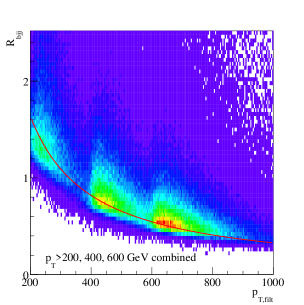
   Figure 9: $R_{\text{opt}}^{\text{(calc)}}$ fit based on Standard Model $t\bar{t}$ samples with $p_{T,t}>200,400,600$ GeV for the parton level distance of decay products $R_{bjj}$. The fat jets are filtered with $R=0.2$, $N=10$. The functional form of the fit curve is given in Eq.(15).

9. in the $N$-subjettiness mode heptop4 compute the $\tau_{j}$ nsubjettiness as defined in Eq.(7) from the filtered and unfiltered subjets, as described below. Again, this mode is not part of our tagger code and relies on the FastJet Contrib fastjet ; fastjet_contrib add-on for $N$–subjettiness nsubjettiness .

10. in the Qjets mode replace the deterministic output of step 1 by a set of possible histories defined in Eq.(10); run the tagger for each of them, giving a set of clustering histories with global weights $\Omega$, and a positive or negative tagging result.

Following this description the low-$p_{T}$ (7) and $N$-subjettiness (9) modes simply add kinematic observables to the tagger output. These observables can be included in a multivariate analysis or can be cut on in the deterministic top tagging decision. The improvement in the low-$p_{T}$ mode is illustrated in detail in Ref. heptop4 while the impact of $N$-subjettiness variables on the resonance search is illustrated in Fig. 6.

In contrast, the optimalR mode and the Qjets mode modify the clustering histories (1) underlying the mass drop search (2). Depending on the modified fat jet size or on the Qjets weight they return a set of tagging outputs. For the optimalR mode it is straightforward to choose the smallest reasonable fat jet size $R_{\text{opt}}$ for the actual tagging. The Qjets histories can be evaluated in a range of possible ways.

Performance

Figure 10: Performance of the HEPTopTagger2 for $t\bar{t}$ production in the Standard Model. We show the incremental improvements from the extended multivariate analyses for top quarks with $p_{T,t}>200~{}\text{GeV}$ and $p_{T,t}>600~{}\text{GeV}$.

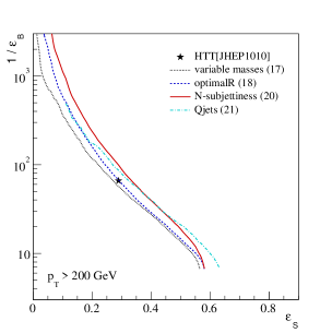
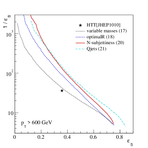
The main body of this paper focuses on $t\bar{t}$ resonance searches using the HEPTopTagger described above. While the combination of tagged top kinematics and fat jet kinematics in Sec.II does not directly translate into to a universal top tagger, the multivariate aspects discussed in Sec. III, namely optimalR, $N$-subjettiness, and Qjets do. Here, we show efficiencies for extracting $t\bar{t}$ events from the QCD multi-jet background.

Our analyses are based on fully hadronic $t\bar{t}$ signal and QCD dijet background samples generated with Pythia8 pythia . For the general top tagger analysis in this Appendix we include underlying event in the event generation and mimic the limited detector resolution by clustering the hadronic activity into $\eta\times\phi$ cells of size $0.1\times 0.1$, similar to the Qjets results shown in Fig. 6. Instead of the hard acceptance cuts in Eq.(1) we now allow for softer fat jets. Two multivariate BDT analyses focus on $t\bar{t}$ samples with

$$p_{T,\text{fat}}>200~{}\text{GeV}\qquad\qquad|y_{\text{fat}}|<2.5\qquad\qquad p_{T,t}>200,600~{}\text{GeV}\;,$$ (16)

where the top momenta are evaluated on the Monte Carlo truth level. We select events with fat C/A jets of radius $R_{\text{fat}}=1.8$ and $|y_{\text{fat}}|<2.5$ constructed with FastJet.

Background efficiencies $\varepsilon_{B}$ are defined as relative to the number of those fat jets. For the signal efficiencies we require that the fat jets can be matched to a parton level top quark within $\Delta R<0.8$. Using the original version of the HEPTopTagger heptop2 we find for the $p_{T}>600$ GeV samples a signal efficiency of $\varepsilon_{S}=35.6\%$ and a mis-tagging rate $\varepsilon_{B}=2.7\%$. The first change in the algorithm addresses the signal efficiency and background sculpting. In the original algorithm the triplet of subjets closest to the true top mass is selected and only later the mass plane cuts are applied. Therefore, the tagger will fail if this triplet does not pass the mass plane constraints and no alternative triplet is analyzed. To eliminate this limitation, we first apply the mass plane constraints and then pick the triple closest to the top mass, as described above.

As in the main text we study further improvements of the tagger based on ROC curves. To allow for such improvements we loosen the cuts of the tagger to $m_{\text{rec}}<1$ TeV and $f_{W}=0.3$. The initial set of BDT parameters in analogy to Eq.(4) is

$$\{\ m_{\text{rec}},f_{\text{rec}}\ \}\;\qquad\qquad\text{(variable masses).}$$ (17)

The large cone size of $R=1.8$ is not always appropriate, so the optimalR mode optimizes the radius of each fat jet. Starting from the initial cone size we stepwise reduce the size of the fat jet until the criterion Eq.(5) indicates that we miss a top decay jet. For the last stable $R$ size we run the usual tagging algorithm. We can calculate the expected value $R_{\text{opt}}^{\text{calc}}$ for the critical radius based on the transverse momentum of the filtered fat jet. For a fat jet originating from a top decay this prediction should agree with the measured value, while for a background fat jet the two are only strongly correlated when the entire subjet kinematics is a perfect match to a top decay. For the optimalR mode we set up a BDT analysis with the observables

$$\{\ m_{\text{rec}},f_{\text{rec}},R_{\text{opt}}-R_{\text{opt}}^{(\text{calc})}\ \}\qquad\qquad\text{(optimalR).}$$ (18)

All tagging observables are evaluated for a fat jet with size $R_{\text{opt}}$. In Fig. 10 we show the improvement from the optimized size of the fat jet. Obviously, it is more impressive for larger boost, while for $p_{T,t}>200$ GeV the optimalR mode hardly leads to a reduction in fat jet size.

The $N$-subjettiness variables are best applied independently for fat jets which would pass and would not pass the initial tagging criterion. The optimalR working point

$$m_{\text{rec}}\in[150,200]~{}\text{GeV}\qquad\qquad f_{\text{rec}}<0.175\qquad\qquad R_{\text{opt}}-R_{\text{opt}}^{(\text{calc})}<0.3\;,$$ (19)

which corresponds to the signal efficiency $\varepsilon_{S}=0.22(0.27)$ in Fig. 10, defines these two categories. Fat jets passing Eq.(19) can be assumed to include a complete set of top decay products and are filtered with $R_{\text{filt}}^{(1)}=0.2$ and $N_{\text{filter}}^{(1)}=5$; fat jets failing this criterion are instead filtered with $R_{\text{filt}}^{(0)}=0.3$ and $N_{\text{filter}}^{(0)}=3$. The unfiltered $N$-subjettiness variables $\tau_{i}$ defined in Eq.(7) and their filtered counter parts $\tau^{(0)}_{i},\tau_{i}^{(1)}$ are included up to $i\leq 3$. The reference axes are chosen as $k_{T}$-axes. We then set up two independent BDTs with

$$\{\ m_{\text{rec}},f_{\text{rec}},R_{\text{opt}}-R_{\text{opt}}^{(\text{calc})},m_{\text{fat}}^{(1)},\tau^{(1)}_{3},\tau^{(1)}_{3}/\tau^{(1)}_{2},\tau^{(1)}_{2}/\tau^{(1)}_{1},\tau_{2},\tau_{3}/\tau_{2},\tau_{2}/\tau_{1}\ \}\qquad\text{($N$-subjettiness, pass)}$$

$$\{\ m_{\text{rec}},f_{\text{rec}},R_{\text{opt}}-R_{\text{opt}}^{(\text{calc})},m_{\text{fat}}^{(0)},\tau^{(0)}_{3},\tau^{(0)}_{3}/\tau^{(0)}_{2},\tau^{(0)}_{2}/\tau^{(0)}_{1},\tau_{1},\tau_{3}/\tau_{2},\tau_{2}/\tau_{1}\ \}\qquad\text{($N$-subjettiness, fail),}$$ (20)

and later combine them into one ROC curve. This precise condition is represented by the more generic Eq.(8). In Fig. 10 we show the corresponding ROC curves for a successively improved tagger.

Finally, we can replace the deterministic clustering history from the usual jet algorithm with a set of Qjets histories with large global weights $\Omega^{(\alpha)}$ defined in Eq.(10) for $\alpha=0.1$. This way we avoid cases where the deterministic clustering history entering the top tagging algorithm is misled during the independent evaluation of splittings in the usual jet algorithm. When defining jets as analysis objects for a hard process this does not pose a problem, but for subjet analyses it can have an effect.

	$t\bar{t}$	QCD
default HTT	0.337	0.0212
$\varepsilon_{\text{Qjets}}>0.1$	0.435	0.0318
$\varepsilon_{\text{Qjets}}>0.2$	0.384	0.0231
$\varepsilon_{\text{Qjets}}>0.3$	0.341	0.0174
$\varepsilon_{\text{Qjets}}>0.4$	0.298	0.0123
$\varepsilon_{\text{Qjets}}>0.5$	0.250	0.0089
$\varepsilon_{\text{Qjets}}>0.6$	0.212	0.0064
$\varepsilon_{\text{Qjets}}>0.7$	0.163	0.0036
$\varepsilon_{\text{Qjets}}>0.8$	0.118	0.0021
$\varepsilon_{\text{Qjets}}>0.9$	0.064	0.0007

	$t\bar{t}$	QCD
default HTT	0.465	0.0489
$\varepsilon_{\text{Qjets}}>0.1$	0.524	0.0661
$\varepsilon_{\text{Qjets}}>0.2$	0.447	0.0461
$\varepsilon_{\text{Qjets}}>0.3$	0.388	0.0342
$\varepsilon_{\text{Qjets}}>0.4$	0.336	0.0245
$\varepsilon_{\text{Qjets}}>0.5$	0.281	0.0168
$\varepsilon_{\text{Qjets}}>0.6$	0.236	0.0118
$\varepsilon_{\text{Qjets}}>0.7$	0.181	0.0062
$\varepsilon_{\text{Qjets}}>0.8$	0.133	0.0032
$\varepsilon_{\text{Qjets}}>0.9$	0.069	0.0009

Table 3: Tagging efficiencies for $p_{T}>200$ GeV (left) and $p_{T}>600$ GeV (right). $\varepsilon_{\text{Qjets}}$ is defined as the number of Qjets tags per number of Qjets runs. For this table we test 10.000 fat jets with 100 Qjets iterations.

Our analysis is based on 100 Qjets histories per fat jet. In Tab. 3 we show their signal and background efficiency if required to lead to individual top tags. As the reference value we use the default HEPTopTagger with fixed mass windows. Based on 100 Qjets histories we then define the fraction $\varepsilon_{\text{Qjets}}$ of histories which lead to a top tag with the default tagging setup. We see that for moderately boosted tops the deterministic signal tagging efficiency can be reproduced by requiring $30\%$ of the Qjets histories to deliver a positive tag. The corresponding mis-tag probability is slightly reduced compared to the deterministic tagger. For harder tops the corresponding value is around $\varepsilon_{\text{Qjets}}>20\%$, with no improvement in the background rejection.

Figure 11: Performance of the HEPTopTagger2 for $t\bar{t}$ production in the Standard Model. For $p_{T,t}>200~{}\text{GeV}$ and $p_{T,t}>600~{}\text{GeV}$ we we focus on different Qjets setups, based on a more basic multivariate tagger without optimalR and $N$-subjettiness.

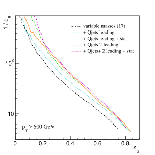
As discussed in Sec. III Qjets offers two strategies to improve the top tagger. To maximize the improvement in the tagging performance and to limit the CPU time we base the multivariate analysis on the tagged history with the largest global weight. As additional parameters we include the value of $\varepsilon_{\text{Qjets}}$ as well as the mean and variance of the $m_{\text{rec}}$ distribution with the 100 Qjets entries, symbolically denoted as $\{m_{\text{rec}}^{\text{Qjets}}\}$. For the BDT analysis the variables are

$$\{\ m_{\text{rec}},f_{\text{rec}},R_{\text{opt}}-R_{\text{opt}}^{(\text{calc})},m_{\text{fat}},\tau_{N},\tau_{N}^{\text{(filt)}},\varepsilon_{\text{Qjets}},\{m_{\text{rec}}^{\text{Qjets}}\}\;\}\qquad\text{({Qjets})}$$ (21)

As usual, all variables from the tagger are evaluated for the optimized $R$ size and the clustering history with the largest global weight. The additional improvement is shown in Fig. 10.

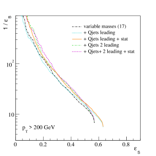
Because Qjets offers a variety of improvements to the tagger, we study different setups based on the stage with multivariate mass windows in Fig. 11. We start by replacing the deterministic C/A output with the most likely Qjets history and including $\varepsilon_{\text{Qjets}}$ in the multivariate analysis. This leads to a moderate improvement of the tagger at large transverse momenta and at large signal efficiencies. Adding the statistical information from the $\varepsilon_{\text{Qjets}}\times 100$ entries in the $m_{\text{rec}}$ information leads to a sizeable improvement over a wide range of signal efficiencies. This is the mode we use for the $Z^{\prime}$ analysis as well as in Fig. 10.

Next, we add the second-best Qjets history to the tagger, such that the multivariate tagger (including $\varepsilon_{\text{Qjets}}$) is free to construct a criterion based on one or two tags in the two best Qjets histories. For most of the ROC curves this comparably simple approach is as successful as the full statistical information. Finally, adding the statistical information on the $m_{\text{rec}}$ distribution leads to a mild improvement.

Interface

To apply the HEPTopTagger algorithm to a fat C/A jet constructed with FastJet3 fastjet , the only necessary steps are executing the default constructor HEPTopTagger(fastjet::PseudoJet jet) followed by running the tagger using void run(). This will analyze the fat jet using the optimalR procedure with the default settings given in Tab. 5. The available operation modes are shown in Tab. 4. All configurable parameters are listed in Tab. 5. Functions to retrieve results are presented in Tab. 6.

QHTT() sets up the Qjets mode. It is applied to a fully configured HEPTopTagger by void run(HEPTopTagger htt). All configurable parameters are given in Tab. 7. A list of functions to access the results is presented in Tab. 8.

In addition, we provide a framework for the calculation of Fox–Wolfram moments that relies on an existing installation of GSL gsl . While the constructor FWM(vector<fastjet::PseudoJet> jets) allows the calculation of Fox–Wolfram moments for a given set of jets, FWM(HEPTopTagger htt, unsigned selection) uses the $b$, $W_{1}$, and $W_{2}$ momenta from the HEPTopTagger run and calculates the Fox–Wolfram moments in the top rest frame. The boost axis $\vec{a}$ itself can be included heptop4 . Subsets of these four vectors can be set via unsigned selection, as a sequence of 0 or 1 in the order $abW_{1}W_{2}$. In Tab. 9 we show how to extract the Fox–Wolfram moment of a given order of the Legendre polynomials.

Finally, we include an example class LowPt() for a fixed low-$p_{T}$ mode working point returning a tagging decision including the set low-$p_{T}$ mode by is_tagged(HEPTopTagger).

name	description
EARLY_MASSRATIO_SORT_MASS	apply the 2D mass plane requirements, then select the candidate which minimizes $|m_{\text{cand}}-m_{t}|$
LATE_MASSRATIO_SORT_MASS	select the candidate which minimizes $|m_{\text{cand}}-m_{t}|$
EARLY_MASSRATIO_SORT_MODDJADE	apply the 2D mass plane requirements, then select the candidate with the highest modified Jade distance
LATE_MASSRATIO_SORT_MODDJADE	select the candidate with the highest modified Jade distance
TWO_STEP_FILTER	only analyze the candidate built with the highest $p_{T,t}$ after unclustering

Table 4: HEPTopTagger working modes.

name	default	description
general:
do_optimalR(bool)	true	use optimalR approach
unclustering:
set_mass_drop_threshold(double)	0.8	mass drop threshold
set_max_subjet_mass(double)	30	max subjet mass for unclustering
filtering:
set_filtering_R(double)	0.3	max subjet distance for filtering
set_filtering_n(unsigned)	5	max subjet number for filtering
set_filtering_minpt_subjet(double)	0.	min subjet $p_{T}$ for filtering
set_filtering_jetalgorithm(          fastjet::JetAlgorithm)	cambridge_algorithm	jet algorithm for filtering
reclustering:
set_reclustering_jetalgorithm(          fastjet::JetAlgorithm)	cambridge_algorithm	jet algorithm for reclustering
candidate selection:
set_mode(enum)	EARLY_MASSRATIO_SORT_MASS	run mode, see Tab. 4
set_mt(double)	172.3	true top mass
set_mw(double)	80.4	true W mass
set_top_mass_range(double, double)	150, 200	top mass window
set_fw(double)	0.15	width of A–shaped bands $f_{W}$
set_mass_ratio_range(          double, double)	$(1-f_{W})\,m_{W}/m_{t}=0.397$ $(1+f_{W})\,m_{W}/m_{t}=0.537$	width of cut in 2D mass plane
set_mass_ratio_cut(double,          double, double)	0.35, 0.2, 1.3	boundaries in 2D mass plane
set_top_minpt(double)	200	min $p_{T,t}$ consistency cut
pruning:
set_pruning_zcut(double)	0.1	$z_{\text{cut}}$ for pruned mass $m_{\text{prune}}$
set_pruning_rcut_factor(double)	0.5	$r_{\text{cut}}$ for pruned mass $m_{\text{prune}}$
optimalR:
set_optimalR_max(double)	size of the input fat jet	max jet size
set_optimalR_min(double)	0.5	min jet size
set_optimalR_step(double)	0.1	step size (multiple of 0.1)
set_optimalR_threshold(double)	0.2	optimalR mass threshold
calculation of $R_{\text{opt}}^{\text{(calc)}}$:
set_filtering_optimalR_calc_R(double)	0.2	max subjet distance for filtering
set_filtering_optimalR_calc_n(unsigned)	10	max subjet number for filtering
set_optimalR_calc_fun(double (*f)(double))	$327/p_{T,\text{filt}}$	dependency of $R_{\text{opt}}^{\text{(calc)}}$ on $p_{T,\text{filt}}$
optimalR type:
set_optimalR_type_top_mass_range(double, double)	150. 200.	mass range for optimalR type 1
set_optimalR_type_f_rec(double)	0.175	max $f_{\text{rec}}$ for optimalR type 1
set_optimalR_type_max_diff(double)	0.3	max $R_{\text{opt}}-R_{\text{opt}}^{\text{(calc)}}$ for optimalR type 1
$N$-subjettiness:
set_filtering_optimalR_pass_R(double)	0.2	$R_{\text{filt}}$ for optimalR type 1
set_filtering_optimalR_pass_n(unsigned)	5	$N_{\text{filt}}$ optimalR type 1
set_filtering_optimalR_fail_R(double)	0.3	$R_{\text{filt}}$ for optimalR type 0
set_filtering_optimalR_fail_n(unsigned)	3	$N_{\text{filt}}$ for optimalR type 0

Table 5: Additional parameters of the HEPTopTagger algorithm. All functions have a return type of void.

name	description
bool is_maybe_top()	top mass window requirement passed?
bool is_masscut_passed()	2D mass plane requirements passed?
bool is_minptcut_passed()	candidate $p_{T,t}$ threshold passed?
bool is_tagged()	top mass window, 2D mass plane requirement, and $p_{T,t}$ threshold passed?
double delta_top()	$|m_{\text{rec}}-m_{t}|$
double djsum()	modified Jade distance
double pruned_mass()	pruned top mass
double unfiltered_mass()	mass of the triplet of subjets after unclustering before filtering
double f_rec()	minimal $|(m_{ij}/m_{\text{rec}})/(m_{W}/m_{t})-1|$
const PseudoJet & t()	top candidate 4-vector
const PseudoJet & b()	subjet corresponding to the $b$
const PseudoJet & W()	combined subjets corresponding to the $W$
const PseudoJet & W1()	leading subjet from the $W$
const PseudoJet & W2()	sub-leading subjet from the $W$
const std::vector<PseudoJet> & top_subjets()	three subjets from the top, ordered: $b$, $W_{1}$, $W_{2}$
const PseudoJet & j1()	leading subjet
const PseudoJet & j2()	sub-leading subjet
const PseudoJet & j3()	sub-sub-leading subjet
const std::vector<PseudoJet> & top_hadrons()	all top constituents
const std::vector<PseudoJet> & hardparts()	hard subtructures after unclustering, sorted by $p_{T}$
const PseudoJet & fat_inital()	original fat jet (after Qjets reclustering)
const PseudoJet & fat_Ropt()	fat jet reduced to $R_{\text{opt}}$
void get_setting()	print settings to stdout
void get_info()	print tagger information to stdout
HEPTopTagger HTTagger(unsigned i)	HEPTopTagger candidate for a distance parameter $R=i/10$. By default all functions above return values at $R=R_{\text{opt}}$. This function accesses candidates for different values of $R$.
double Ropt()	$R_{\text{opt}}$
double Ropt_calc()	$R_{\text{opt}}^{\text{(calc)}}$
int optimalR_type()	result of set optimalR working point. 1 = pass, 0 = fail
double nsub_unfiltered(int order, fastjet::contrib::Njettiness::AxesMode axes = fastjet::contrib::Njettiness::kt_axes, double beta = 1., double R0 = 1.);	$N$–subjettiness $\tau_{i}$ for the unfiltered fat jet
double nsub_filtered(int order, fastjet::contrib::Njettiness::AxesMode axes = fastjet::contrib::Njettiness::kt_axes, double beta = 1., double R0 = 1.);	$N$–subjettiness $\tau^{\text{(filt)}}_{i}$ for the fat jet after filtering depending on optimalR_type().
double q_weight()	weight of used Qjets history

Table 6: Functions to retrieve results of the HEPTopTagger algorithm.

name	default	description
set_iterations(unsigned)	100	number of Qjets iterations
set_q_zcut(double)	0.1	$z_{\text{cut}}$ for pruning in Qjets
set_q_dcut_fctr(double)	0.5	$D_{\text{cut}}$ factor for pruning in Qjets
set_q_exp(double a, double b)	0., 0. (C/A)	set distance measure for Qjets $d_{ij}=\min(p_{T,i},p_{T,j})^{a}\,\max(p_{T,i},p_{T,j})^{b}\,R_{ij}^{2}$
set_q_rigidity(double)	0.1	rigidity $\alpha$ for Qjets
set_q_truncation_fctr(double)	0.	threshold for merging probability $\omega_{ij}$ in Qjets

Table 7: Parameters of the Qjets frame for the HEPTopTagger. All functions have a return type of void.

name	description
HEPTopTagger leading()	HEPTopTagger with leading tagged history
HEPTopTagger subleading()	HEPTopTagger with subleading tagged history
double weight_leading()	Qjets weight of the leading tagged history
double weight_subleading()	Qjets weight of the subleading tagged history
double eps_q()	$\varepsilon_{\text{Qjets}}$
double m_mean()	$\langle m\rangle$ for the tagged histories
double m2_mean()	$\langle m^{2}\rangle$ for the tagged histories

Table 8: Functions to retrieve results of the Qjets frame.

name	description
double U(unsigned)	FWM of given order with unit weight
double Pt(unsigned, fastjet::PseudoJet=$(0.,0.,1.,0.)$)	FWM of given order with $p_{T}$ weight relative to the given reference vector.

Table 9: Functions to retrieve Fox–Wolfram moments.

References

- (1) D. E. Morrissey, T. Plehn and T. M. P. Tait, Phys. Rept. 515, 1 (2012).
- (2) see e.g. K. Agashe, A. Belyaev, T. Krupovnickas, G. Perez and J. Virzi, Phys. Rev. D 77, 015003 (2008) V. Barger, T. Han and D. G. E. Walker, Phys. Rev. Lett. 100, 031801 (2008); B. Lillie, L. Randall and L. -T. Wang, JHEP 0709, 074 (2007); U. Baur and L. H. Orr, Phys. Rev. D 76, 094012 (2007); U. Baur and L. H. Orr, Phys. Rev. D 77, 114001 (2008); P. Fileviez Perez, R. Gavin, T. McElmurry and F. Petriello, Phys. Rev. D 78, 115017 (2008).
- (3) ATLAS Collaboration, JHEP 1301, 116 (2013); ATLAS Collaboration, ATLAS-CONF-2013-084; ATLAS Collaboration, ATLAS-CONF-2012-102. G Piacquadio CERN-THESIS-2010-027; G Kasieczka, PhD thesis, http://www.ub.uni-heidelberg.de/archiv/14941.
- (4) T. Plehn, G. P. Salam and M. Spannowsky, Phys. Rev. Lett. 104, 111801 (2010);
- (5) T. Plehn, M. Spannowsky, M. Takeuchi, and D. Zerwas, JHEP 1010, 078 (2010); http://www.thphys.uni-heidelberg.de/~plehn/index.php?show=heptoptagger&visible=tools
- (6) L. G. Almeida, S. J. Lee, G. Perez, I. Sung and J. Virzi, Phys. Rev. D 79, 074012 (2009); L. G. Almeida, S. J. Lee, G. Perez, G. F. Sterman, I. Sung and J. Virzi, Phys. Rev. D 79, 074017 (2009); L. G. Almeida, S. J. Lee, G. Perez, G. Sterman, I. Sung, Phys. Rev. D82, 054034 (2010); M. Backovic and J. Juknevich, Comput. Phys. Commun. 185, 1322 (2014).
- (7) for a review see e.g. A. Abdesselam et al., Eur. Phys. J. C 71, 1661 (2011); T. Plehn and M. Spannowsky, J. Phys. G 39, 083001 (2012); A. Altheimer et al., arXiv:1311.2708 [hep-ex]; S. Schaetzel, arXiv:1403.5176 [hep-ex].
- (8) M. H. Seymour, Z. Phys. C 62, 127 (1994); J. M. Butterworth, B. E. Cox and J. R. Forshaw, Phys. Rev. D 65, 096014 (2002).
- (9) W. Skiba and D. Tucker-Smith, Phys. Rev. D 75, 115010 (2007); B. Holdom, JHEP 0703, 063 (2007). M. Gerbush, T. J. Khoo, D. J. Phalen, A. Pierce and D. Tucker-Smith, Phys. Rev. D 77, 095003 (2008); G. Brooijmans, ATL-PHYS-CONF-2008-008 and ATL-COM-PHYS-2008-001, Feb. 2008.
- (10) M. Dasgupta, A. Fregoso, S. Marzani and G. P. Salam, JHEP 1309, 029 (2013).
- (11) J. M. Butterworth, A. R. Davison, M. Rubin and G. P. Salam, Phys. Rev. Lett. 100, 242001 (2008).
- (12) D. E. Kaplan, K. Rehermann, M. D. Schwartz and B. Tweedie, Phys. Rev. Lett. 101, 142001 (2008).
- (13) for a promising new key observable, see A. J. Larkoski, S. Marzani, G. Soyez and J. Thaler, JHEP 1405, 146 (2014)
- (14) for an extension beyond the usual fat jet approach see M. Stoll, arXiv:1410.4637 [hep-ph].
- (15) C. Anders, C. Bernaciak, G. Kasieczka, T. Plehn and T. Schell, arXiv:1312.1504 [hep-ph].
- (16) D. E. Soper and M. Spannowsky, Phys. Rev. D 87, 054012 (2013);
- (17) D. E. Soper and M. Spannowsky, Phys. Rev. D 89, no. 9, 094005 (2014).
- (18) M. R. Buckley, T. Plehn and M. Takeuchi, JHEP 1308, 086 (2013); M. R. Buckley, T. Plehn, T. Schell and M. Takeuchi, JHEP 1402, 130 (2014).
- (19) T. Plehn and M. Takeuchi, J. Phys. G 38, 095006 (2011).
- (20) T. Plehn, M. Spannowsky and M. Takeuchi, Phys. Rev. D 85, 034029 (2012).
- (21) S. D. Ellis, C. K. Vermilion and J. R. Walsh, Phys. Rev. D 80, 051501 (2009); S. D. Ellis, C. K. Vermilion and J. R. Walsh, Phys. Rev. D 81, 094023 (2010); C. K. Vermilion, arXiv:1101.1335 [hep-ph].
- (22) Y. L. Dokshitzer, G. D. Leder, S. Moretti and B. R. Webber, JHEP 9708, 001 (1997); M. Wobisch and T. Wengler, arXiv:hep-ph/9907280.
- (23) S. Catani, Y. L. Dokshitzer, M. Olsson, G. Turnock and B. R. Webber, Phys. Lett. B 269, 432 (1991); S. Catani, Y. L. Dokshitzer, M. H. Seymour and B. R. Webber, Nucl. Phys. B 406, 187 (1993); S. D. Ellis and D. E. Soper, Phys. Rev. D 48, 3160 (1993).
- (24) M. Cacciari and G. P. Salam, Phys. Lett. B 641, 57 (2006); M. Cacciari, G. P. Salam and G. Soyez, Eur. Phys. J. C 72, 1896 (2012); http://fastjet.fr
- (25) G. C. Fox and S. Wolfram, Phys. Rev. Lett. 41, 1581 (1978); C. Bernaciak, M. S. A. Buschmann, A. Butter and T. Plehn, Phys. Rev. D 87, 073014 (2013); C. Bernaciak, B. Mellado, T. Plehn, X. Ruan, and P. Schichtel, arXiv:1311.5891 [hep-ph].
- (26) S. D. Ellis, A. Hornig, T. S. Roy, D. Krohn and M. D. Schwartz, Phys. Rev. Lett. 108, 182003 (2012); S. D. Ellis, A. Hornig, D. Krohn and T. S. Roy, arXiv:1409.6785 [hep-ph].
- (27) Y. T. Chien, Phys. Rev. D 90, 054008 (2014).
- (28) F. Kling, T. Plehn and M. Takeuchi, Phys. Rev. D 86, 094029 (2012).
- (29) T. Sjöstrand, S. Ask, J. R. Christiansen, R. Corke, N. Desai, P. Ilten, S. Mrenna and S. Prestel et al., arXiv:1410.3012 [hep-ph].
- (30) A. Höcker et al., PoS ACAT , 040 (2007) [physics/0703039 [PHYSICS]]; P. Speckmayer, A. Höcker, J. Stelzer and H. Voss, J. Phys. Conf. Ser. 219, 032057 (2010); http://tmva.sourceforge.net
- (31) D. Krohn, J. Thaler and L. T. Wang, JHEP 0906, 059 (2009).
- (32) J. Thaler and K. Van Tilburg, JHEP 1103, 015 (2011); J. Thaler and K. Van Tilburg, JHEP 1202, 093 (2012); I. W. Stewart, F. J. Tackmann and W. J. Waalewijn, Phys. Rev. Lett. 105, 092002 (2010).
- (33) for a possible improvement over -subjettiness see A. J. Larkoski, I. Moult and D. Neill, JHEP 1412, 009 (2014); A. J. Larkoski, I. Moult and D. Neill, Phys. Rev. D 91, no. 3, 034035 (2015).
- (34) for an alternative new approach see e.g. M. Freytsis, T. Volansky and J. R. Walsh, arXiv:1412.7540 [hep-ph].
- (35) T. Strebler, Master thesis, ETH Zürich (2014)
- (36) see e.g. C. Englert, T. Plehn, P. Schichtel and S. Schumann, Phys. Rev. D 83, 095009 (2011); S. Ask, J. H. Collins, J. R. Forshaw, K. Joshi and A. D. Pilkington, JHEP 1201, 018 (2012); E. Gerwick, T. Plehn, S. Schumann and P. Schichtel, JHEP 1210, 162 (2012); E. Gerwick, S. Schumann, B. Gripaios and B. Webber, JHEP 1304, 089 (2013); Z. Bern, L. J. Dixon, F. Febres Cordero, S. Höche, H. Ita, D. A. Kosower, D. Maitre and K. J. Ozeren, Phys. Rev. D 88, no. 1, 014025 (2013).
- (37) for some early examples see e.g. K. Kondo, J. Phys. Soc. Jap. 57, 4126 (1988); D. Atwood and A. Soni, Phys. Rev. D 45, 2405 (1992); V. M. Abazov et al. [D0 Collaboration], Phys. Lett. B 617, 1 (2005); A. Abulencia et al. [CDF Collaboration], Phys. Rev. D73, 092002 (2006); V.M Abazov et. al. [D0 Collaboration], Nature 429, 638 (2004).
- (38) http://fastjet.hepforge.org/contrib/
- (39) http://www.gnu.org/software/gsl/