Kinetically Modified Non-Minimal Chaotic Inflation

Abstract

Abstract: We consider Supersymmetric (SUSY) and non-SUSY models of chaotic inflation based on the $\phi^{n}$ potential with $2\leq n\leq 6$. We show that the coexistence of a non-minimal coupling to gravity $f_{\cal R}=1+c_{\cal R}\phi^{n/2}$ with a kinetic mixing of the form $f_{\rm K}=c_{\rm K}f_{\cal R}^{m}$ can accommodate inflationary observables favored by the Bicep2/Keck Array and Planck results for $0\leq m\leq 4$ and $2.5\cdot 10^{-4}\leq r_{\mathcal{R}\rm K}=c_{\cal R}/c_{\rm K}^{n/4}\leq 1,$ where the upper limit is not imposed for $n=2$. Inflation can be attained for subplanckian inflaton values with the corresponding effective theories retaining the perturbative unitarity up to the Planck scale.

PACs numbers: 98.80.Cq, 04.50.Kd, 12.60.Jv, 04.65.+e Published in Phys. Rev. D 91, 123508 (2015)

I Introduction

It is well-known old ; nmi ; roest that the presence of a non-minimal coupling function

$$f_{\cal R}(\phi)=1+c_{\cal R}\phi^{n/2},$$ (1)

between the inflaton $\phi$ and the Ricci scalar $\mathcal{R}$, considered in conjunction with a monomial potential of the type

$$V_{\rm CI}(\phi)=\lambda^{2}\phi^{n}/2^{n/2},$$ (2)

provides, at the strong $c_{\cal R}$ limit with $\phi<1$ – in the reduced Planck units with $m_{\rm P}=M_{\rm P}/\sqrt{8\pi}=1$ –, an attractor roest towards the spectral index, $n_{\rm s}$, and the tensor-to-scalar ratio, $r$, respectively

$$n_{\rm s}\simeq 1-2/{\widehat{N}_{\star}}=0.965~{}~{}\mbox{and}~{}~{}r\simeq 12/{\widehat{N}_{\star}}^{2}=0.0036,$$ (3)

for ${\widehat{N}_{\star}}=55$ e-foldings with negligible $n_{\rm s}$ running, $a_{\rm s}$. Although perfectly consistent with the present combined Bicep2/Keck Array and Planck results plcp ; gws ,

$$n_{\rm s}=0.968\pm 0.0045~{}~{}\mbox{and}~{}~{}r=0.048^{+0.035}_{-0.032},$$ (4)

$r$ in Eq. (3) lies well below its central value in Eq. (4) and the sensitivity of the present experiments searching for primordial gravity waves – for an updated survey see cmbpol . Nonetheless, this model – called henceforth non-minimal chaotic inflation (MCI) – exhibits also a weak $c_{\cal R}$ regime, with $\phi>1$ and $c_{\cal R}$-dependent observables roest ; oss approaching for decreasing $c_{\cal R}$’s their values within MCI chaotic . Focusing on this regime, we would like to emphasize that solutions covering nicely the 1-$\sigma$ domain of the present data in Eq. (4) can be achieved, even for $\phi<1$, by introducing a suitable non-canonical kinetic mixing $f_{\rm K}(\phi)$. For this reason we call this type of non-MCI kinetically modified. Although a new parameter $c_{\rm K}$, included in $f_{\rm K}$, may take relatively high values within this scheme, no problem with the perturbative unitarity arises.

II non-SUSY Framework

Non-MCI is formulated in the Jordan frame (JF) where the action of $\phi$ is given by

$${\sf S}=\int d^{4}x\sqrt{-\mathfrak{g}}\left(-\frac{f_{\cal R}}{2}\mathcal{R}+\frac{f_{\rm K}}{2}g^{\mu\nu}\partial_{\mu}\phi\partial_{\nu}\phi-V_{\rm CI}(\phi)\right).$$ (5)

Here $\mathfrak{g}$ is the determinant of the background Friedmann-Robertson-Walker metric, $g^{\mu\nu}$ with signature $(+,-,-,-)$ and we allow for a kinetic mixing through the function $f_{\rm K}(\phi)$. By performing a conformal transformation nmi according to which we define the Einstein frame (EF) metric $\widehat{g}_{\mu\nu}=f_{\cal R}\,g_{\mu\nu}$ we can write ${\sf S}$ in the EF as follows

$${\sf S}=\int d^{4}x\sqrt{-\widehat{\mathfrak{g}}}\left(-\frac{1}{2}\widehat{\mathcal{R}}+\frac{1}{2}\widehat{g}^{\mu\nu}\partial_{\mu}\widehat{\phi}\partial_{\nu}\widehat{\phi}-\widehat{V}_{\rm CI}(\widehat{\phi})\right),$$ (6a)

where hat is used to denote quantities defined in the EF. We also introduce the EF canonically normalized field, $$\widehat{\phi} \widehat{V}_{\rm CI}$$, and potential, , defined as follows:

$$\frac{d\widehat{\phi}}{d\phi}=J=\sqrt{\frac{f_{\rm K}}{f_{\cal R}}+{3\over 2}\left({f_{\cal R,\phi}\over f_{\cal R}}\right)^{2}}~{}~{}~{}\mbox{and}~{}~{}~{}\widehat{V}_{\rm CI}=\frac{V_{\rm CI}}{f_{\cal R}^{2}}\,,$$ (6b)

where the symbol $,\phi$ as subscript denotes derivation with respect to (w.r.t) the field $\phi$. In the pure non-MCI old ; nmi ; roest we take $f_{\rm K}=1$ and so, as shown from Eq. (6b), the role of $f_{\cal R}$ in Eq. (1) is twofold:

• it determines the canonical normalization of $\widehat{\phi}$; and

• it controls the shape of $\widehat{V}_{\rm CI}$ affecting thereby the observational predictions.

Inspired by Ref. takahashi ; lee , where non-canonical kinetic terms assist in obtaining inflationary solutions for $\phi<1$, we liberate $f_{\cal R}$ from its first role above implementing it by a kinetic function of the form

$$f_{\rm K}(\phi)=c_{\rm K}f_{\cal R}^{m}~{}~{}\mbox{where}~{}~{}c_{\rm K}=(c_{\cal R}/r_{\mathcal{R}\rm K})^{4/n},$$ (7)

with $r_{\mathcal{R}\rm K}$ being introduced for later convenience. The form of $f_{\rm K}$ in Eq. (7) is chosen so that the perturbative unitarity is preserved up to Planck scale. Its most general form could be $f_{\rm K}=c_{\rm K}\tilde{f}$ with $\tilde{f}$ being an arbitrary function such that $\tilde{f}(\langle{\phi}\rangle=0)=1$ – see below. However, the variation of $f_{\rm K}$ generated by $\tilde{f}$ can be covered by the parametrization of Eq. (7) selecting conveniently $m=\ln\tilde{f}/\ln f_{\cal R}$.

Plugging, finally, Eqs. (7) and (2) into Eq. (6b) we obtain

$$J^{2}=\frac{c_{\rm K}}{f_{\cal R}^{1-m}}+\frac{3n^{2}c_{\cal R}^{2}\phi^{n-2}}{8f_{\cal R}^{2}}\simeq\frac{c_{\rm K}}{f_{\cal R}^{1-m}}~{}~{}\mbox{and}~{}~{}\widehat{V}_{\rm CI}=\frac{\lambda^{2}\phi^{n}}{2^{n/2}f_{\cal R}^{2}},$$ (8)

assuming $c_{\rm K}\gg c_{\cal R}$. In contrast to Ref. lee the presence of both $f_{\rm K}$ and $f_{\cal R}$ plays a crucial role within our proposal.

III Supergravity Embeddings

The supersymmetrization of the above models requires the use of two gauge singlet chiral superfields, i.e., $z^{\alpha}=\Phi,S$, with $\Phi$ (${\alpha}=1$) and $S$ (${\alpha}=2)$ being the inflaton and a “stabilized” field respectively. The EF action for $z^{\alpha}$’s within Supergravity (SUGRA) linde1 can be written as

$${\sf S}=\int d^{4}x\sqrt{-\widehat{\mathfrak{g}}}\left(-\frac{1}{2}\widehat{\mathcal{R}}+K_{{\alpha}{\bar{\beta}}}\widehat{g}^{\mu\nu}\partial_{\mu}z^{\alpha}\partial_{\nu}z^{*{\bar{\beta}}}-\widehat{V}\right)$$ (9a)

where summation is taken over the scalar fields $$z^{\alpha} K K_{{\alpha}{\bar{\beta}}}=K_{,z^{\alpha}z^{*{\bar{\beta}}}} K^{{\alpha}{\bar{\beta}}}K_{{\bar{\beta}}\gamma}=\delta^{\alpha}_{\gamma} \widehat{V}$$, star (^∗) denotes complex conjugation, is the Kähler potential with and . Also is the EF F–term SUGRA potential given by

$$\widehat{V}=e^{K}\left(K^{{\alpha}{\bar{\beta}}}(D_{\alpha}W)(D^{*}_{\bar{\beta}}W^{*})-3{|W|^{2}}\right),$$ (9b)

where $D_{\alpha}W=W_{,z^{\alpha}}+K_{,z^{\alpha}}W$ with $W$ being the superpotential. Along the inflationary track determined by the constraints

$$S=\Phi-\Phi^{*}=0,~{}\mbox{or}~{}~{}s=\bar{s}={\theta}=0$$ (10)

if we express $\Phi$ and $S$ according to the parametrization

$$\Phi=\>{\phi\,e^{i{\theta}}}/{\sqrt{2}}\>\>\>\mbox{and}\>\>\>S=\>(s+i\bar{s})/\sqrt{2}\,,$$ (11)

$V_{\rm CI}$ in Eq. (2) can be produced, in the flat limit, by

$$W=\lambda S\Phi^{n/2}.$$ (12)

The form of $W$ can be uniquely determined if we impose two symmetries:

• an $R$ symmetry under which $S$ and $\Phi$ have charges $1$ and $0$;

• a global $U(1)$ symmetry with assigned charges $-1$ and $2/n$ for $S$ and $\Phi$.

On the other hand, the derivation of $\widehat{V}_{\rm CI}$ in Eq. (8) via Eq. (9b) requires a judiciously chosen $K$. Namely, along the track in Eq. (10) the only surviving term in Eq. (9b) is

$$\widehat{V}_{\rm CI}=\widehat{V}({\theta}=s=\bar{s}=0)=e^{K}K^{SS^{*}}\,|W_{,S}|^{2}\,.$$ (13)

The incorporation $f_{\cal R}$ in Eq. (1) and $f_{\rm K}$ in Eq. (7) dictates the adoption of a logarithmic $K$ linde1 including the functions

$$F_{\cal R}(\Phi)=1+2^{\frac{n}{4}}\Phi^{\frac{n}{2}}c_{\cal R}~{}~{}\mbox{and}~{}~{}F_{\rm K}=(\Phi-\Phi^{*})^{2}\,.$$ (14a)

Here $$F_{\cal R} f_{\cal R} F_{\rm K} f_{\rm K} F_{\rm K} \widehat{V}_{\rm CI} \Phi |\Phi|^{2}/3 J \widehat{V}_{\rm CI} F_{\rm K} K S$$is an holomorphic function reducing to , along the path in Eq. (10), and is a real function which assists us to incorporate the non-canonical kinetic mixing generating by in Eq. (7). Indeed, lets intact , since it vanishes along the trajectory in Eq. (10), but it contributes to the normalization of – contrary to the naive kinetic term linde1 which influences both and in Eq. (6b). Although is employed in Ref. roest too, its importance in implementing non-minimal kinetic terms within non-MCI has not been emphasized so far. We also include in the typical kinetic term for , considering the next-to-minimal term for stability reasons linde1 – see below –, i.e.

$$F_{S}={|S|^{2}/3}-k_{S}{|S|^{4}/3}.$$ (14b)

Taking for consistency all the possible terms up to fourth order, $K$ is written as

$$K=-3\ln\left(\frac{c_{\rm K}}{2^{m}6}\left(F_{\cal R}+F_{\cal R}^{*}\right)^{m}F_{\rm K}\right.$$

$$\left.+\frac{1}{2}\left(F_{\cal R}+F_{\cal R}^{*}\right)-F_{S}+\frac{k_{\Phi}}{6}F_{\rm K}^{2}-\frac{k_{S\Phi}}{3}F_{\rm K}{|S|^{2}}\right)\,.~{}~{}~{}~{}~{}$$ (15a)

Alternatively, if we do not insist on a pure logarithmic $$K$$, we could also adopt the form

$$K=-3\ln\left(\frac{1}{2}\left(F_{\cal R}+F_{\cal R}^{*}\right)-F_{S}\right)-\frac{c_{\rm K}}{2^{m}}\frac{F_{\rm K}}{\left(F_{\cal R}+F_{\cal R}^{*}\right)^{1-m}}\,\cdot$$ (15b)

Note that for $m=0$ [$m=1$], $F_{\rm K}$ and $F_{\cal R}$ in $K$ given by Eq. (15a) [Eq. (15b)] are totally decoupled, i.e. no higher order term is needed. Our models, for $c_{\rm K}\gg c_{\cal R}$, are completely natural in the ’t Hooft sense because, in the limits $c_{\cal R}\rightarrow 0$ and $\lambda\rightarrow 0$, the theory enjoys the following enhanced symmetries – cf. Ref. shift :

$$\Phi\rightarrow\ \Phi^{*},\>\Phi\rightarrow\ \Phi+c\>\>\>\mbox{and}\>\>\>S\rightarrow\ e^{i\alpha}S,$$ (16)

where $c$ is a real number. Therefore, the terms proportional to $c_{\cal R}$ can be regarded as a gravity-induced violation of the symmetries above.

To verify the appropriateness of $K$ in Eqs. (15a) and (15b), we can first remark that, along the trough in Eq. (10), it is diagonal with non-vanishing elements $K_{\Phi\Phi^{*}}=J^{2}$, where $J$ is given by Eq. (8), and $K_{SS^{*}}=1/f_{\cal R}$. Upon substitution of $K^{SS^{*}}=f_{\cal R}$ and $\exp K=f_{\cal R}^{-3}$ into Eq. (13) we easily deduce that $\widehat{V}_{\rm CI}$ in Eq. (8) is recovered. If we perform the inverse of the conformal transformation described in Eqs. (6a) and (5) with frame function ${\Omega/3}=-\exp\left(-{K}/{3}\right)$ we end up with the JF potential $V_{\rm CI}=\Omega^{2}\widehat{V}_{\rm CI}/9$ in Eq. (2). Moreover, the conventional Einstein gravity at the SUSY vacuum, $\langle{S}\rangle=\langle{\Phi}\rangle=0$, is recovered since $-\langle{\Omega}\rangle/3=1$.

Table 1: Mass spectrum along the path in Eq. (10).

Fields	Eingestates	Mass Squared
$1$ real scalar	$\widehat{\theta}$	$\widehat{m}^{2}_{{\theta}}\simeq n_{\theta}\widehat{V}_{\rm CI}/3=n_{\theta}\widehat{H}_{\rm CI}^{2}$
$2$ real scalars	$\widehat{s},\widehat{\bar{s}}$	$\widehat{m}^{2}_{s}\simeq 2(6k_{S}f_{\cal R}-1)\widehat{H}_{\rm CI}^{2}$
$2$ Weyl spinors	$({\widehat{\psi}_{S}\pm\widehat{\psi}_{\Phi})/\sqrt{2}}~{}~{}$	$\widehat{m}^{2}_{\psi\pm}\simeq 3n^{2}\widehat{H}_{\rm CI}^{2}/2c_{\rm K}\phi^{2}f_{\cal R}^{1+m}$

Defining the canonically normalized fields via the relations

$${d\widehat{}\phi/d\phi}=\sqrt{K_{\Phi\Phi^{*}}}=J,\>\>\>\widehat{{\theta}}=J{\theta}\phi,$$ (17)

and $(\widehat{s},\widehat{\bar{s}})=\sqrt{K_{SS^{*}}}{(s,\bar{s})}$ we can verify that the configuration in Eq. (10) is stable w.r.t the excitations of the non-inflaton fields. Taking the limit $c_{\rm K}\gg c_{\cal R}$ we find the expressions of the masses squared $\widehat{m}^{2}_{\chi^{\alpha}}$ (with $\chi^{\alpha}={\theta}$ and $s$) arranged in Table 1, which approach rather well the quite lengthy, exact expressions taken into account in our numerical computation. These expressions assist us to appreciate the role of $k_{S}>0$ in retaining positive $\widehat{m}^{2}_{s}$. Also we confirm that $\widehat{m}^{2}_{\chi^{\alpha}}\gg\widehat{H}_{\rm CI}^{2}=\widehat{V}_{\rm CI0}/3$ for $\phi_{\rm f}\leq\phi\leq\phi_{\star}$ – note that $n_{\theta}=4$ or $6$ for $K$ taken by Eq. (15a) or Eq. (15b), respectively. In Table 1 we display the masses $\widehat{m}^{2}_{\psi^{\pm}}$ of the corresponding fermions too. We define $\widehat{\psi}_{S}=\sqrt{K_{SS^{*}}}\psi_{S}$ and $\widehat{\psi}_{\Phi}=\sqrt{K_{\Phi\Phi^{*}}}\psi_{\Phi}$ where $\psi_{\Phi}$ and $\psi_{S}$ are the Weyl spinors associated with $S$ and $\Phi$ respectively.

Inserting the derived mass spectrum in the well-known Coleman-Weinberg formula, we can find the one-loop radiative corrections, $\Delta\widehat{V}_{\rm CI}$ to $\widehat{V}_{\rm CI}$. It can be verified that our results are immune from $\Delta\widehat{V}_{\rm CI}$, provided that the renormalization group mass scale $\Lambda$, is determined by requiring $\Delta\widehat{V}_{\rm CI}(\phi_{\star})=0$ or $\Delta\widehat{V}_{\rm CI}(\phi_{\rm f})=0$. The possible dependence of our results on the choice of $\Lambda$ can be totally avoided if we confine ourselves to $k_{S\Phi}\sim 1$ and $k_{S}\sim(0.5-1.5)$ resulting to $\Lambda\simeq(4-20)\cdot 10^{-5}$ – cf. Ref. nmi ; nIG . Under these circumstances, our results in the SUGRA set-up can be exclusively reproduced by using $\widehat{V}_{\rm CI}$ in Eq. (8).

IV Inflation Analysis

The period of slow-roll non-MCI is determined in the EF by the condition:

$${\footnotesize\sf max}\{\widehat{\epsilon}(\phi),|\widehat{\eta}(\phi)|\}\leq 1,$$ (18a)

where the slow-roll parameters $$\widehat{\epsilon} \widehat{\eta}$$ and read

$$\widehat{\epsilon}=\left({\widehat{V}_{\rm CI,\widehat{\phi}}/\sqrt{2}\widehat{V}_{\rm CI}}\right)^{2}\>\>\>\mbox{and}\>\>\>\>\>\widehat{\eta}={\widehat{V}_{\rm CI,\widehat{\phi}\widehat{\phi}}/\widehat{V}_{\rm CI}}$$ (18b)

and can be derived employing $J$ in Eq. (6b), without express explicitly $\widehat{V}_{\rm CI}$ in terms of $\widehat{\phi}$. Our results are

$$\widehat{\epsilon}=\frac{n^{2}}{2\phi^{2}c_{\rm K}f_{\cal R}^{1+m}};~{}~{}\frac{\widehat{\eta}}{\widehat{\epsilon}}=2\left(1-\frac{1}{n}\right)-\frac{4+n(1+m)}{2n}c_{\cal R}\phi^{\frac{n}{2}}\,.$$ (19)

Given that $\phi\ll 1$ and so $f_{\cal R}\simeq 1$, Eq. (18a) is saturated at the maximal $\phi$ value, $\phi_{\rm f}$, from the following two values

$$\phi_{1\rm f}\simeq{n/\sqrt{2c_{\rm K}}}\>\>\>\mbox{and}\>\>\>\phi_{2\rm f}\simeq\sqrt{(n-1)n/c_{\rm K}},$$ (20)

where $\phi_{1\rm f}$ and $\phi_{2\rm f}$ are such that $\widehat{\epsilon}\left(\phi_{1\rm f}\right)\simeq 1$ and $\widehat{\eta}\left(\phi_{2\rm f}\right)\simeq 1$.

Table 2: Inflationary predictions for $n=4$ and $m=1,2,$ and $4$.

	$m=1$	$m=2$	$m=4$
$n_{\rm s}$	$1-3/2{\widehat{N}_{\star}}-3/8({\widehat{N}_{\star}}^{3}r_{\mathcal{R}\rm K})^{1/2}$	$1-4/3{\widehat{N}_{\star}}-1/2(3{\widehat{N}_{\star}}^{4}r_{\mathcal{R}\rm K})^{1/3}$	$1-6/5{\widehat{N}_{\star}}-3/5(40{\widehat{N}_{\star}}^{6}r_{\mathcal{R}\rm K})^{1/5}-3/10(50{\widehat{N}_{\star}}^{7}r_{\mathcal{R}\rm K}^{2})^{1/5}$
$r$	$1/2{\widehat{N}_{\star}}^{2}r_{\mathcal{R}\rm K}+2/({\widehat{N}_{\star}}^{3}r_{\mathcal{R}\rm K})^{1/2}$	$8/3(3{\widehat{N}_{\star}}^{4}r_{\mathcal{R}\rm K})^{1/3}+4/3(9{\widehat{N}_{\star}}^{5}r_{\mathcal{R}\rm K}^{2})^{1/3}$	$8(4/5{\widehat{N}_{\star}}^{6}r_{\mathcal{R}\rm K})^{1/5}/5+4(16/25{\widehat{N}_{\star}}^{7}r_{\mathcal{R}\rm K}^{2})^{1/5}/5$
$a_{\rm s}$	$-3/2{\widehat{N}_{\star}}^{2}-9/16({\widehat{N}_{\star}}^{5}r_{\mathcal{R}\rm K})^{1/2}$	$-4/3{\widehat{N}_{\star}}^{2}-2/3(3{\widehat{N}_{\star}}^{7}r_{\mathcal{R}\rm K})^{1/3}$	$-6/5{\widehat{N}_{\star}}^{2}-9(4/5{\widehat{N}_{\star}}^{11}r_{\mathcal{R}\rm K})^{1/5}/25$

The number of e-foldings ${\widehat{N}_{\star}}$ that the scale $k_{\star}=0.05/{\rm Mpc}$ experiences during this non-MCI and the amplitude $A_{\rm s}$ of the power spectrum of the curvature perturbations generated by $\phi$ can be computed using the standard formulae

$${\widehat{N}_{\star}}=\int_{\widehat{\phi}_{\rm f}}^{\widehat{\phi}_{\star}}d\widehat{\phi}\frac{\widehat{V}_{\rm CI}}{\widehat{V}_{\rm CI,\widehat{\phi}}}~{}~{}\mbox{and}~{}~{}A_{\rm s}^{1/2}=\frac{1}{2\sqrt{3}\,\pi}\;\frac{\widehat{V}_{\rm CI}^{3/2}(\widehat{\phi}_{\star})}{|\widehat{V}_{\rm CI,\widehat{\phi}}(\widehat{\phi}_{\star})|},$$ (21)

where $\phi_{\star}~{}[\widehat{\phi}_{\star}]$ is the value of $\phi~{}[\widehat{\phi}]$ when $k_{\star}$ crosses the inflationary horizon. Since $\phi_{\star}\gg\phi_{\rm f}$, from Eq. (21) we find

$${\widehat{N}_{\star}}=\frac{c_{\rm K}\phi_{\star}^{2}}{2n}\;{}_{2}F_{1}\left(-m,4/n;1+4/n;-c_{\cal R}\phi_{\star}^{n/2}\right),$$ (22)

where ${}_{2}F_{1}$ is the Gauss hypergeometric function wolfram which reduces to unity for $m=0$ (and any $n$) or to the factor $(f_{\cal R}^{1+m}-1)/\phi_{\star}^{2}c_{\cal R}(1+m)$ for $n=4$ (and any $m$). Concetrating on these cases, we solve Eq. (22) w.r.t $\phi_{\star}$ with result

$$\phi_{\star}\simeq\begin{cases}\sqrt{2n{\widehat{N}_{\star}}/c_{\rm K}}~{}~{}\mbox{for}~{}~{}m=0,\\ \sqrt{f_{m\star}-1}/\sqrt{r_{\mathcal{R}\rm K}c_{\rm K}}~{}~{}\mbox{for}~{}~{}n=4,\end{cases}$$ (23)

where $f_{m\star}^{1+m}=1+8(m+1)r_{\mathcal{R}\rm K}{\widehat{N}_{\star}}$. In both cases there is a lower bound on $c_{\rm K}$, above which $\phi_{\star}<1$ and so, our proposal can be stabilized against corrections from higher order terms. From Eq. (21) we can also derive a constraint on $\lambda$ and $c_{\rm K}$ i.e.

$$\lambda=\sqrt{3A_{\rm s}}\pi\cdot\begin{cases}\left(c_{\rm K}/n{\widehat{N}_{\star}}\right)^{\frac{n}{4}}\left(2nf_{n\star}/{\widehat{N}_{\star}}\right)^{\frac{1}{2}}~{}~{}\mbox{for}~{}~{}m=0,\\ 16c_{\rm K}r_{\mathcal{R}\rm K}^{3/2}/(f_{m\star}-1)^{\frac{3}{2}}f_{m\star}^{\frac{m-1}{2}}~{}~{}\mbox{for}~{}~{}n=4\end{cases}$$ (24)

where $f_{n\star}=f_{\cal R}(\phi_{\star})=1+r_{\mathcal{R}\rm K}(2n{\widehat{N}_{\star}})^{n/4}$.

The inflationary observables are found from the relations

$$n_{\rm s}=\>1-6\widehat{\epsilon}_{\star}\ +\ 2\widehat{\eta}_{\star},~{}~{}r=16\widehat{\epsilon}_{\star},$$ (25a)

$$a_{\rm s}=\>2\left(4\widehat{\eta}_{\star}^{2}-(n_{\rm s}-1)^{2}\right)/3-2\widehat{\xi}_{\star},$$ (25b)

where the variables with subscript $\star$ are evaluated at $\phi=\phi_{\star}$ and $\widehat{\xi}={\widehat{V}_{\rm CI,\widehat{\phi}}\widehat{V}_{\rm CI,\widehat{\phi}\widehat{\phi}\widehat{\phi}}/\widehat{V}^{2}_{\rm CI}}$. For $m=0$ we find

$$n_{\rm s}=1-\left(4+n+n/f_{n\star}\right)/4{\widehat{N}_{\star}},~{}~{}r=4n/f_{n\star}{\widehat{N}_{\star}},~{}~{}~{}~{}~{}~{}~{}~{}~{}~{}~{}~{}$$ (26a)

$$a_{\rm s}=\big{(}n^{2}-n(n+4)f_{n\star}-4(n+4)f_{n\star}^{2}\big{)}/16f_{n\star}^{2}{\widehat{N}_{\star}}^{2}\,.~{}~{}~{}$$ (26b)

In the limit $r_{\mathcal{R}\rm K}\rightarrow 0$ or $f_{n\star}\rightarrow 1$ the results of the simplest power-law MCI, Eq. (2), are recovered – cf. Ref. chaotic . The formulas above are also valid for the original non-MCI roest with $c_{\rm K}=1$ and $r_{\mathcal{R}\rm K}=c_{\cal R}$ lower than the one needed to reach the attractor’s values in Eq. (3). In this limit our results are in agreement with those displayed in Ref. oss for $n=4$. Furthermore, for $n=4$ (and any $m$) we obtain

$$n_{\rm s}=1-8r_{\mathcal{R}\rm K}\frac{m-1+(m+2)f_{m\star}}{(f_{m\star}-1)f_{m\star}^{1+m}},$$ (27a)

$$r=\frac{128r_{\mathcal{R}\rm K}}{(f_{m\star}-1)f_{m\star}^{1+m}},~{}~{}a_{\rm s}=\frac{64r_{\mathcal{R}\rm K}^{2}(1+m)(m+2)}{(f_{m\star}-1)^{2}f_{m\star}^{4(1+m)}}\cdot$$

$$f_{m\star}^{2}\left(f_{m\star}^{2m}\left(\frac{1-m}{m+2}+\frac{2m-1}{m+1}f_{m\star}\right)-f_{m\star}^{2(1+m)}\right).~{}~{}~{}$$ (27b)

For $n=4$ and $m=1,2$ and $4$ the outputs of Eqs. (26a)-(27b) are specified in Table 2 after expanding the relevant formulas for $1/{\widehat{N}_{\star}}\ll 1$. We can clearly infer that increasing $m$ for fixed $r_{\mathcal{R}\rm K}$, both $n_{\rm s}$ and $r$ increase. Note that this formulae, based on Eq. (23), is valid only for $r_{\mathcal{R}\rm K}>0$ (and $m\neq 0$).

From the analytic results above, see Eq. (24) and Eqs. (26a) – (27b), we deduce that the free parameters of our models, for fixed $n$ and $m$, are $r_{\mathcal{R}\rm K}$ and $\lambda/c_{\rm K}^{n/4}$ and not $c_{\rm K}$, $c_{\cal R}$ and $\lambda$ as naively expected. This fact can be understood by the following observation: If we perform a rescaling $\phi=\tilde{}\phi/\sqrt{c_{\rm K}}$, Eq. (5) preserves its form replacing $\phi$ with $\tilde{}\phi$ and $f_{\rm K}$ with $f_{\cal R}^{m}$ where $f_{\cal R}$ and $V_{\rm CI}$ take, respectively, the forms

$$f_{\cal R}=1+r_{\mathcal{R}\rm K}\tilde{}\phi^{n/2}~{}~{}\mbox{and}~{}~{}V_{\rm CI}=\lambda^{2}\tilde{}\phi^{n}/2^{n/2}c_{\rm K}^{n/2},$$ (28)

which, indeed, depend only on $r_{\mathcal{R}\rm K}$ and $\lambda^{2}/c_{\rm K}^{n/2}$.

The conclusions above can be verified and extended to others $n$’s and $m$’s numerically. In particular, confronting the quantities in Eq. (21) with the observational requirements plcp

$${\widehat{N}_{\star}}\simeq 55~{}~{}\mbox{and}~{}~{}A_{\rm s}^{1/2}\simeq 4.627\cdot 10^{-5},$$ (29)

we can restrict $\lambda/c_{\rm K}^{n/4}$ and $\phi_{\star}$ and compute the model predictions via Eqs. (25a) and (25b), for any selected $m,n$ and $r_{\mathcal{R}\rm K}$. The outputs, encoded as lines in the $n_{\rm s}-r_{0.002}$ plane, are compared against the observational data plcp ; gws in Fig. 1 for $m=0,1,2,$ and $4$ and $n=2$ (dashed lines), $n=4$ (solid lines), and $n=6$ (dot-dashed lines). The variation of $r_{\mathcal{R}\rm K}$ is shown along each line. To obtain an accurate comparison, we compute $r_{0.002}=16\widehat{\epsilon}(\phi_{0.002})$ where $\phi_{0.002}$ is the value of $\phi$ when the scale $k=0.002/{\rm Mpc}$, which undergoes $\widehat{N}_{0.002}=({\widehat{N}_{\star}}+3.22)$ e-foldings during non-MCI, crosses the horizon of non-MCI.

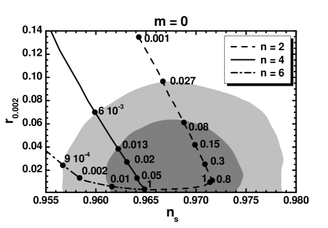
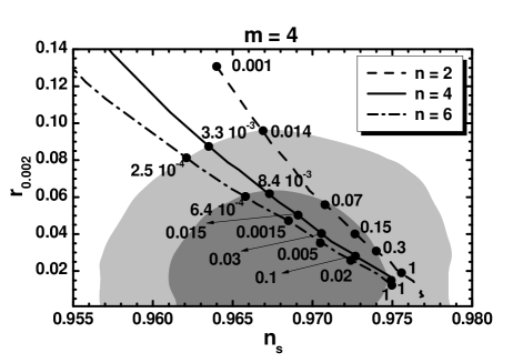
Fig. 1: Allowed curves in the $n_{\rm s}-r_{0.002}$ plane for $m=0,1,2$ and $4$, $n=2$ (dashed lines), $n=4$ (solid lines), $n=6$ (dot-dashed lines) and various $r_{\mathcal{R}\rm K}$’s indicated on the curves. The marginalized joint $68\%$ [$95\%$] regions from Planck, Bicep2/Keck Array and BAO data are depicted by the dark [light] shaded contours.

From the plots in Fig. 1 we observe that, for low enough $r_{\mathcal{R}\rm K}$’s – i.e. $r_{\mathcal{R}\rm K}=10^{-7},10^{-4},$ and $0.001$ for $n=6,4,$ and $2$ –, the various lines converge to the $(n_{\rm s},r_{0.002})$’s obtained within MCI. At the other end, the lines for $n=4$ and $6$ terminate for $r_{\mathcal{R}\rm K}=1$, beyond which the theory ceases to be unitarity safe – see below – whereas the $n=2$ line approaches an attractor value for any $m$. For $m=0$ we reveal the results of Ref. roest , i.e. the displayed lines are almost parallel for $r_{0.002}\geq 0.02$ and converge at the values in Eq. (3) – for $n=4$ and $6$ this is reached even for $r_{\mathcal{R}\rm K}=1$. For $m>0$ the curves move to the right and span more densely the 1-$\sigma$ ranges in Eq. (4) for quite natural $r_{\mathcal{R}\rm K}$’s – e.g. $0.005\lesssim r_{\mathcal{R}\rm K}\lesssim 0.1$ for $m=1$ and $n=4$. It is worth mentioning that the requirement $r_{\mathcal{R}\rm K}\leq 1$ provides a lower bound on $r_{0.002}$, which ranges from $0.0032$ (for $m=0$ and $n=6$) to $0.015$ (for $m=4$ and $n=4$). Note, finally, that our estimations in Eqs. (26a)–(26b) are in agreement with the numerical results for $n=2$ and $r_{\mathcal{R}\rm K}\lesssim 1$, $n=6~{}[4]$ and $r_{\mathcal{R}\rm K}\lesssim 0.002~{}[0.05]$. For $m>0$ (and $n=4$) our findings in Eqs. (27a)–(27b) (and Table 2) approximate fairly the numerical outputs for $0.003\lesssim r_{\mathcal{R}\rm K}\leq 1$.

V Effective Cut-Off Scale

The selected $f_{\rm K}$ in Eq. (7) not only reconciles non-MCI with the 1-$\sigma$ ranges in Eq. (4) but also assures that the corresponding effective theories respect perturbative unitarity up to $m_{\rm P}=1$ although $c_{\rm K}$ may take relatively large values for $\phi<1$ – e.g. for $n=4,m=1$ and $r_{\mathcal{R}\rm K}=0.03$ we obtain $140\lesssim c_{\rm K}\lesssim 1.4\cdot 10^{6}$ for $3.3\cdot 10^{-4}\lesssim\lambda\lesssim 3.5$. This achievement stems from the fact that $\widehat{\phi}=\langle{J}\rangle\phi$ does not coincide – contrary to the pure non-MCI cutoff ; riotto for $n>2$ – with $\phi$ at the vacuum of the theory, given that $\langle{J}\rangle=\sqrt{c_{\rm K}}$ or $\langle{J}\rangle=\sqrt{c_{\rm K}+3c_{\cal R}^{2}/2}$ for $\langle{\phi}\rangle=0$ and $n>2$ or $n=2$ – see Eq. (8). It is notable that this by-product of our proposal for $n>2$ arises without invoking large $\langle{\phi}\rangle$’s as in Ref. nIG ; lee ; gian .

To clarify further this point we analyze the small-field behavior of our models in the EF. We focus on the second term in the right-hand side of Eq. (6a) or (9a) for $\mu=\nu=0$ and we expand it about $\langle{\phi}\rangle=0$ in terms of $\widehat{\phi}$ – see Eq. (6b). Our result for $m=0$ and $n=2,4,$ and $6$ can be written as

$$J^{2}\dot{\phi}^{2}=\left(1-r_{\mathcal{R}\rm K}\widehat{\phi}^{\frac{n}{2}}+\frac{3n^{2}}{8}r_{\mathcal{R}\rm K}^{2}\widehat{\phi}^{n-2}+r_{\mathcal{R}\rm K}^{2}\widehat{\phi}^{n}\cdots\right)\dot{}\widehat{\phi}^{2}.$$ (30)

Similar expressions can be obtained for the other $$m \widehat{V}_{\rm CI} \widehat{\phi}$$’s too. Expanding similarly , see Eq. (8), in terms of we have

$$\widehat{V}_{\rm CI}=\frac{\lambda^{2}\widehat{\phi}^{n}}{2c_{\rm K}^{n/2}}\left(1-2r_{\mathcal{R}\rm K}\widehat{\phi}^{\frac{n}{2}}+3r_{\mathcal{R}\rm K}^{2}\widehat{\phi}^{n}-4r_{\mathcal{R}\rm K}^{3}\widehat{\phi}^{\frac{3n}{2}}+\cdots\right),$$

independently of $m$. From the expressions above we conclude that our models do not face any problem with the perturbative unitarity for $r_{\mathcal{R}\rm K}\leq 1$. For $n=2$ this statement is also valid even for $r_{\mathcal{R}\rm K}>1$ as shown in Ref. nmi ; riotto . In the latter case, though, the naturalness argument mentioned below Eq. (15b) is invalidated.

VI Conclusions

Prompted by the recent joint analysis of Bicep2/Keck Array and Planck which, although does not exclude inflationary models with negligible $r$’s, seems to favor those with $r$’s of order $0.01$ we proposed a variant of non-MCI which can safely accommodate $r$’s of this level. The main novelty of our proposal is the consideration of the non-canonical kinetic mixing in Eq. (7) – involving the parameters $m$ and $c_{\rm K}$ – apart from the non-minimal coupling to gravity in Eq. (1) which is associated with the potential in Eq. (2). This setting can be elegantly implemented in SUGRA too, employing the super- and Kähler potentials given in Eqs. (12) and (15a) or (15b). Prominent in this realization is the role of a shift-symmetric quadratic function $F_{\rm K}$ in Eq. (14a) which remains invisible in the SUGRA scalar potential while dominates the canonical normalization of the inflaton. Using $m\geq 0$ and confining $r_{\mathcal{R}\rm K}$ to the range $(2.5\cdot 10^{-4}-1)$, where the upper bound does not apply to the $n=2$ case, we achieved observational predictions which may be tested in the near future and converge towards the “sweet” spot of the present data – its compatibility with the $m=1$ case, especially for $n=4$ and $6$, is really impressive – see Fig. 1. These solutions can be attained even with subplanckian values of the inflaton requiring large $c_{\rm K}$’s and without causing any problem with the perturbative unitarity. It is gratifying, finally, that a sizable fraction of the allowed parameter space of our models (with $n=4$) can be studied analytically and rather accurately.

Acknowledgments

The author acknowledges useful discussions with G. Lazarides, A. Racioppi, and G. Trevisan. This research was supported from the MEC and FEDER (EC) grants FPA2011-23596 and the Generalitat Valenciana under grant PROMETEOII/2013/017.

References

D. S. Salopek, J. R. Bond and J.M. Bardeen, Phys. Rev. D 40, 1753 (1989); F.L. Bezrukov and M. Shaposhnikov, Phys. Lett. B 659, 703 (2008) [arXiv:0710.3755].

C. Pallis, Phys. Lett. B 692, 287 (2010) [arXiv:1002.4765]; C. Pallis and Q. Shafi, Phys. Rev. D 86, 023523 (2012) [arXiv: 1204.0252]; C. Pallis and Q. Shafi, J. Cosmol. Astropart. Phys. 03, 023 (2015) [arXiv:1412.3757].

R. Kallosh, A. Linde, and D. Roest, Phys. Rev. Lett. 112, 011 303 (2014) [arXiv:1310.3950].

Planck Collaboration, arXiv:1502.02114.

P.A.R. Ade et al. [Bicep2/Keck Array and Planck Collaborations], Phys. Rev. Lett. 114, 101301 (2015) [arXiv:1502. 00612].

P. Creminelli et al., arXiv:1502.01983.

N. Okada, M.U. Rehman, and Q. Shafi, Phys. Rev. D 82, 043502 (2010) [arXiv:1005.5161]; N. Okada, V.N. Şenoğuz, and Q. Shafi, arXiv:1403.6403.

A.D. Linde, Phys. Lett. B 129, 177 (1983).

F. Takahashi, Phys. Lett. B 693, 140 (2010) [arXiv:1006. 2801]; K. Nakayama and F. Takahashi, J. Cosmol. Astropart. Phys. 11, 009 (2010) [arXiv:1008.2956].

H.M. Lee, Eur. Phys. J. C 74, 3022 (2014) [arXiv:1403. 5602].

M.B. Einhorn and D.R.T. Jones, J. High Energy Phys. 03, 026 (2010) [arXiv:0912.2718]; H.M. Lee, J. Cosmol. Astropart. Phys. 08, 003 (2010) [arXiv:1005.2735]; S. Ferrara et al., Phys. Rev. D 83, 025008 (2011) [arXiv:1008.2942]; C. Pallis and N. Toumbas, J. Cosmol. Astropart. Phys. 02, 019 (2011) [arXiv:1101.0325].

R. Kallosh, A. Linde, and T. Rube, Phys. Rev. D 83, 043507 (2011) [arXiv:1011.5945].

C. Pallis, J. Cosmol. Astropart. Phys. 04, 024 (2014) [arXiv: 1312.3623]; C. Pallis, J. Cosmol. Astropart. Phys. 08, 057 (2014) [arXiv:1403.5486]; C. Pallis, J. Cosmol. Astropart. Phys. 10, 058 (2014) [arXiv:1407.8522].

http://functions.wolfram.com.

J.L.F. Barbon and J.R. Espinosa, Phys. Rev. D 79, 081302 (2009) [arXiv:0903.0355]; C.P. Burgess, H.M. Lee, and M. Trott, J. High Energy Phys. 07, 007 (2010) [arXiv:1002. 2730].

A. Kehagias, A.M. Dizgah, and A. Riotto, Phys. Rev. D 89, 043527 (2014) [arXiv:1312.1155].

G.F. Giudice and H.M. Lee, Phys. Lett. B 733, 58 (2014) [arXiv:1402.2129].