NMR investigation of contextuality in a quantum harmonic oscillator
via pseudospin mapping

Abstract

Physical potentials are routinely approximated to harmonic potentials so as to analytically solve the system dynamics. Often it is important to know when a quantum harmonic oscillator (QHO) behaves quantum mechanically and when classically. Recently Su et. al. [Phys. Rev. A 85, 052126 (2012)] have theoretically shown that QHO exhibits quantum contextuality (QC) for a certain set of pseudospin observables. In this work, we encode the four eigenstates of a QHO onto four Zeeman product states of a pair of spin-1/2 nuclei. Using the techniques of NMR quantum information processing, we then demonstrate the violation of a state-dependent inequality arising from the noncontextual hidden variable model, under specific experimental arrangements. We also experimentally demonstrate the violation of a state-independent inequality by thermal equilibrium states of nuclear spins, thereby assessing their quantumness.

I Introduction

Quantum contextuality (QC) states that the outcome of the measurement depends not only on the system and the observable but also on the context of the measurement, i.e., on other compatible observables which are measured along with Peres (1990, 1991, 1995); Kochen and Specker (1967).

Let us consider a pair of space-like separated entangled particles, with local observables $A$ and $C$ belonging to the first particle, and $B$ and $D$ to the second. We assume that these observables are dichotomic (i.e., can take values $\pm 1$) and that the pairs $(A,B),~{}(B,C),~{}(C,D),$ and $(D,A)$ commute.

Classically, one assigns objective properties to the particles such that $D$ behaves identically on the state of the system irrespective of whether it is measured in the context of $A$ or in the context of $C$, even though $A$ and $C$ are not compatible Mermin (1990); Einstein et al. (1935). Such measurements are said to be context independent. Classically, one can pre-assign values $(a,c)$ to $(A,C)$ of the first particle independent of the measurement carried out on the second particle. Similarly, for the second particle one can pre-assign values $(b,d)$ to $(B,D)$ independent of the measurement carried out on the first particle. In these pre-assignments, implicit is the assumption of noncontextual hidden variables, which predict definite measurement outcomes independent of measuring arrangement. If we pre-assign values to observables such that $A,B,C,D=\pm 1$, it follows that $AB+BC+CD-AD=\pm 2$ and the expectation value,

I $$=\langle{AB+BC+CD-AD}\rangle$$ (1)

$$=\langle{AB}\rangle+\langle{BC}\rangle+\langle{CD}\rangle-\langle{AD}\rangle\leq 2$$

Nielsen and Chuang (2010). This inequality often known as CHSH inequality arises from noncontextual hidden variable (NCHV) model and must be satisfied by all classical particles.

Now let us see the implication of the quantum theory. Let Alice and Bob share a large number of singlet states: $(|{01}\rangle-|{10}\rangle)/\sqrt{2}=-(|{+-}\rangle-|{-+}\rangle)/\sqrt{2}$, where $|{0}\rangle$ and $|{1}\rangle$ are eigenkets of Pauli-$z$ operator ($\sigma_{z}$) and $|{\pm}\rangle=(|{0}\rangle\pm|{1}\rangle)/\sqrt{2}$. Alice measures on her qubit either $\sigma_{x}^{A}$ or $\sigma_{z}^{A}$, while Bob always measures $\sigma_{x}^{B}$. Let us compare the results of only those measurements in which Alice has obtained outcome $+1$. If Alice measures $\sigma_{z}^{A}$, then Bob’s qubit collapse to $|{1}\rangle=(|{+}\rangle-|{-}\rangle)/\sqrt{2}$. In this context (i.e., $\sigma_{z}^{A}$), Bob will get both outcomes $\pm 1$ with equal probability. On the other hand, if Alice measures $\sigma_{x}^{A}$ on her qubit, then Bob’s qubit collapses to $|{-}\rangle$ and in this context (i.e., $\sigma_{x}^{A}$), Bob will always get the outcome $-1$. Hence the context dependency.

Here we experimentally investigate QC of a quantum harmonic oscillator (QHO). There are a variety of quantum systems whose potentials are approximated by QHO. Consider for example the quantized electromagnetic field used to manipulate a qubit in cavity quantum electrodynamicsWalther et al (2006). Recently, QC in QHO has been theoretically studied by Su et al Su et. al (2012) by mapping four lowermost QHO states onto four pseudospin states. Such states can be encoded by qubit states, and QC can be studied by realizing the measurements of appropriate observables. We realize this study using a nuclear magnetic resonance (NMR) quantum simulator Cory et. al. (1997) .

In the following section we shall revisit the formulation of Su et al, and in section III, we describe the experimental demonstration of state-dependent and state-independent QC using an NMR system. Finally we conclude in section IV.

II theory

Hong-Yi Su et.al. Su et. al (2012) have theoretically studied QC of eigenstates of $1$D-QHO by introducing two sets of pseudo-spin operators,

$${\bf\Gamma}=(\Gamma_{x},\Gamma_{y},\Gamma_{z}),~{}~{}{\bf\Gamma^{\prime}}=(\Gamma_{x}^{\prime},\Gamma_{y}^{\prime},\Gamma_{z}^{\prime})$$

with components,

$$\Gamma_{x}=\sigma_{x}\otimes\mathbbm{1},\Gamma_{y}=\sigma_{z}\otimes\sigma_{y},\Gamma_{z}=-\sigma_{y}\otimes\sigma_{y},$$

$$\Gamma_{x}^{\prime}=\sigma_{x}\otimes\sigma_{z},\Gamma_{y}^{\prime}=\mathbbm{1}\otimes\sigma_{y},\Gamma_{z}^{\prime}=-\sigma_{x}\otimes\sigma_{x}.$$ (2)

where $\mathbbm{1}$ is $2\times 2$ identity matrix. Using these operators they defined the following observables,

$$A = \Gamma_{x}=\sigma_{x}\otimes\mathbbm{1},$$

$$B = \Gamma_{x}^{\prime}\cos\beta+\Gamma_{z}^{\prime}\sin\beta=\sigma_{x}\otimes(\sigma_{z}\cos\beta-\sigma_{x}\sin\beta),$$

$$C = \Gamma_{z}=-\sigma_{y}\otimes\sigma_{y},$$

$$D = \Gamma_{x}^{\prime}\cos\eta+\Gamma_{z}^{\prime}\sin\eta=\sigma_{x}\otimes(\sigma_{z}\cos\eta-\sigma_{x}\sin\eta).$$ (3)

The products which form the inequality expression (Eq. 1) are

$$AB = \mathbbm{1}\otimes(\cos\beta~{}\sigma_{z}-\sin\beta~{}\sigma_{x}),$$

$$BC = -\sigma_{z}\otimes(\cos\beta~{}\sigma_{x}+\sin\beta~{}\sigma_{z})$$

$$CD = -\sigma_{z}\otimes(\cos\eta~{}\sigma_{x}+\sin\eta~{}\sigma_{z}),$$

$$DA = \mathbbm{1}\otimes(\cos\eta~{}\sigma_{z}-\sin\eta~{}\sigma_{x}).$$ (4)

Following commutation relations hold: $[\Gamma_{i},\Gamma_{j}^{\prime}]=0~{}(i,j=x,y,z)$, $[\Gamma_{x},\Gamma_{y}]=2i~{}\Gamma_{z}$ , $[\Gamma^{\prime}_{x},\Gamma^{\prime}_{y}]=2i~{}\Gamma^{\prime}_{z}$ and cyclic permutation of $x,y,z$. $A,B,C,D$ have eigenvalues $\pm 1$, with $(A,B)$, $(B,C)$, $(C,D)$ and $(D,A)$ forming compatible pairs. $A,~{}B,~{}C$ and $D$ are Hermitian, hence observables. One can verify that they are also unitary operators. Hong-Yi Su et.al. Su et. al (2012) have shown that,

$$\mathrm{\textbf{I}}_{|{l}\rangle_{QHO}}^{QM}=2\sqrt{2}>2,~{}\mathrm{when},~{}(\beta,\eta)_{l}=\begin{cases}(-\pi/4,-3\pi/4)_{0}\\ (3\pi/4,\pi/4)_{1}\\ (\pi/4,3\pi/4)_{2}\\ (-3\pi/4,-\pi/4)_{3}\end{cases}$$ (5)

where, $\mathrm{\textbf{I}}_{|{l}\rangle_{QHO}}^{QM}$ is the expression on LHS of inequality 1, $l=0,1,2\textrm{ and }3$, and, $|{0}\rangle_{QHO},|{1}\rangle_{QHO},|{2}\rangle_{QHO}$ and $|{3}\rangle_{QHO}$ are first four energy eigenstates of 1D-QHO. Thus QHO violates the inequality (1) for certain observables and thereby exhibits QC.

It is well known that only certain two-particle states violate the CHSH inequality (1). As shown in Home (1997); Capasso et al. (1973) factorable states always satisfy inequality (1) for local observables (observables of the form $P\otimes\mathbbm{1}$ or $\mathbbm{1}\otimes Q$ Audretsch (2007)). With maximally mixed state ($\mathbbm{1}\otimes\mathbbm{1}/4$) the inequality (1) is satisfied even with nonlocal observables (observables of the form $P\otimes Q$ Audretsch (2007)) in eq. (3), which is obvious from the fact that all the products in eq. (4) are traceless. However, if the initial state is nonfactorable, we can always find observables such that inequality (1) is violated Home (1997). Although the pseudospin states $\{|{00}\rangle,|{01}\rangle,|{10}\rangle,|{11}\rangle\}$, are factorable, they still violate (1) since the observables in eq. (3) are nonlocal. Thus, we observe that even when a system is in a nonentangled state, measurements of nonlocal observables may lead to violation of noncontextuality inequality Gühne et al (2010).

State independent QC: There exist stronger inequalities obtained from NCHV models which is violated by all states, including separable or maximally mixed states. If the initial state is maximally mixed, entanglement cannot be created by measuring whatever observable (local or nonlocal). This shows that entanglement is not necessary in general even in a bipartite system, to exhibit QC. Hence we conclude that, QC is more fundamental or general than entanglement. Any system whose Hilbert space has dimension $>2$ exhibits QC Kochen and Specker (1967). Even a single spin-1 particle (where entanglement has no meaning as far as spin degree of freedom is concerned) can exhibit QC Kong et al (2012).

III Experiment

III.1 State dependent contextuality

For experimentally studying eq. (1), we need: (i) a physical representation of first four energy eigenstates $\{|{0}\rangle_{QHO},|{1}\rangle_{QHO},|{2}\rangle_{QHO},|{3}\rangle_{QHO}\}$ of 1D-QHO , and (ii) a way to find out the expectation values for operators $AB,~{}BC,~{}CD,$ and $DA$. We encode the first four energy eigenstates of 1D-QHO onto the four energy eigenstates (under secular approximation) of a pair of spin-1/2 nuclei precessing in external static magnetic field: $\{|{00}\rangle,|{01}\rangle,|{10}\rangle,|{11}\rangle\}$, which we call Zeeman product states. In fact any four arbitrarily choosen energy eigenstates of 1D-QHO and also their superposition states exhibit QC Su et. al (2012). The circuit shown in Fig. 1 is called Moussa protocol Moussa et al. (2010), and is used to extract the expectation value of observables in a joint measurement. This has subsequently been generalized by Joshi et al Joshi et al. (2014) to unitary operators.

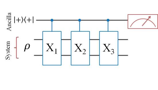
Figure 1: Moussa Protocol for finding out the expectation value of the joint observable $X_{1}X_{2}X_{3}$ i.e. $\langle{X_{1}X_{2}X_{3}}\rangle$. Here $X_{i}$’s are mutually commuting unitary operators.

The three qubits for this experiment were provided by the three ¹⁹F nuclear spins of trifluoroiodoethylene dissolved in acetone-D6. Fig. 2(a) shows the structure of trifluoroiodoethylene along with the Hamiltonian parameters in Fig. 2(b). The effective ¹⁹F spin-spin (T${}_{2}^{*}$) and spin-lattice (T₁) relaxation time constants were about $0.8$ and $6.3$ s respectively. The experiments were carried out at an ambient temperature of 290 K on a 500 MHz Bruker UltraShield NMR spectrometer.

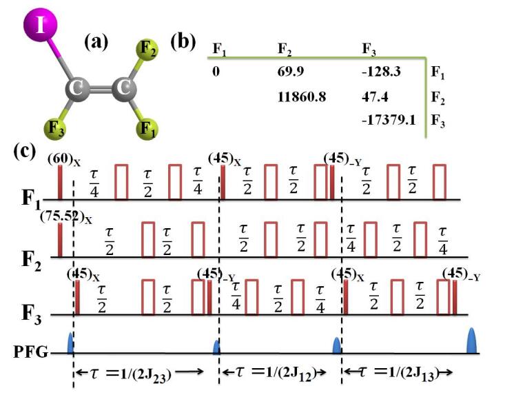
Figure 2: (a) Molecular Structure, (b) chemical shifts(diagonal elements) and J-couplings(off-diagonal elements) in Hz of trifluoroiodoethylene, and (c) pulse sequence for pseudo-pure state preparation. The amplitude and phase of the shaded pulse is written over the top of respective pulse, and unshaded pulses are $(\pi)_{x}$ pulses. During the J evolution $1/(2J_{23})$, $(\pi)_{x}$ pulses refocus $J_{12}$ and $J_{13}$ evolutions and retain only $J_{23}$ evolution. Similarly others. Last row represents Pulsed Field Gradients(PFG), which kills transverse magnetization or in other words they make coefficients of $I_{x}$ and $I_{y}$ zero Cavanagh (1996)

The thermal equilibrium state for the three spin system in the eigenbasis of total Hamiltonian (under secular approximation: $\{|{000}\rangle,|{001}\rangle,...\}$) is

$$\rho_{\mathrm{eq}}=\frac{\mathbbm{1}_{8}}{8}+\epsilon\sum_{i=1}^{3}I_{iz}$$ (6)

where, $\mathbbm{1}_{8}$ is an $8\times 8$ identity matrix, $I_{iz}$ are spin angular momentum operators, and the purity factor $\epsilon=\hbar\omega_{0}/(8kT)$ is the ratio of the Zeeman energy gap to the thermal energy Cavanagh (1996). Unitary operation has no effect on the identity part, but modifies only the traceless deviation part. By applying a series of unitary and nonunitary operators (pulse sequence shown in Fig. 2 Mitra et al. (2008)), it is possible to transform the equilibrium state to a pseudopure state

$$\rho_{\mathrm{pps}}=(1-\epsilon)\frac{\mathbbm{1}_{8}}{8}+\epsilon|{000}\rangle\langle{000}|=\frac{\mathbbm{1}_{8}}{8}+\epsilon\Delta\rho_{|{000}\rangle}$$ (7)

which is isomorphic to the pure state $|{000}\rangle$ Cory et. al. (1997). In the pseudopure state, the traceless deviation part has the form

$$\Delta\rho_{|{000}\rangle}= \frac{1}{4}(I_{1z}+I_{2z}+I_{3z}+2I_{1z}I_{2z}$$ (8)

$$+2I_{2z}I_{3z}+2I_{1z}I_{3z}+4I_{1z}I_{2z}I_{3z}).$$

The first spin, F₁, is used as an ancilla qubit, and other spins, F₂ and F₃, as the system qubits (see Fig. 1). The initial Hadamard gate on the first spin prepares $\rho_{\mathrm{|{+00}\rangle}}$. To measure $\langle{AB}\rangle_{|{00}\rangle}$, we apply the corresponding controlled operations $A$ and $B$ as indicated in circuit 1. The transverse magnetization of the ancilla qubit will be proportional to the expectation value $\langle{AB}\rangle_{|{00}\rangle}$. The absolute value of $\langle{AB}\rangle_{|{00}\rangle}$ is estimated by normalizing the value obtained in the above experiment with that obtained from a reference experiment having no controlled operations. Similarly we can measure the other expectation values $\langle{BC}\rangle_{|{00}\rangle}$, $\langle{CD}\rangle_{|{00}\rangle}$, and $\langle{AD}\rangle_{|{00}\rangle}$, and determine the value of ${\bf I}_{0}$. Other values ${\bf I}_{l}$ are obtained by preparing the corresponding pseudopure states $\rho_{|{+01}\rangle}$, $\rho_{|{+10}\rangle}$, and $\rho_{|{+11}\rangle}$ and applying the circuit 1 in each case.

In our experiments, all the controlled operations were realized by numerically optimized radio frequency (RF) pulses obtained using GRAPE technique Khaneja et. al. (2005). Each pair of controlled operations in circuit 1 was realized by a GRAPE sequence with a duration of about 23 ms (having RF segments of duration $5~{}\upmu s$) and an average Hilbert-Schmidt fidelity better than 0.99 over 10% variation in RF amplitude.

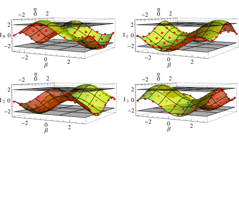
Figure 3: $\mathrm{\textbf{I}}_{0}$,$\mathrm{\textbf{I}}_{1}$,$\mathrm{\textbf{I}}_{2}$,and $\mathrm{\textbf{I}}_{3}$ represents evaluation of expression 1 for eigenstates $|{0}\rangle_{QHO},|{1}\rangle_{QHO},|{2}\rangle_{QHO}$, and $|{3}\rangle_{QHO}$ respectively. The curved surface represents theoretical values, and the points are experimental values. Flat planes at $2$ and $-2$ represents classical bound.

We estimated the values for $\textbf{I}_{l}$ (1), for all the four eigenstates and independently varied both $\beta$ and $\eta$ over the range $[-\pi,\pi]$ with increments of $\pi/4$. The results are shown in Fig. 3. The maximum theoretical violation is $2\sqrt{2}=2.82$. The experimental values of maximum violations for $\textbf{I}_{0}$, $\textbf{I}_{1}$, $\textbf{I}_{2}$, and $\textbf{I}_{3}$ are $2.40\pm 0.02,~{}2.45\pm 0.02,~{}2.39\pm 0.02$, and $2.42\pm 0.03$ respectively.

III.2 State independent contextuality

Hong-Yi Su et.al. also studied the state independent contextuality Su et. al (2012); Cabello (2008). They considered the inequality (arising from NCHV model)

$$\langle{P_{11}P_{12}P_{13}}\rangle+\langle{P_{21}P_{22}P_{23}}\rangle+\langle{P_{31}P_{32}P_{33}}\rangle$$

$$+\langle{P_{11}P_{21}P_{31}}\rangle+\langle{P_{12}P_{22}P_{32}}\rangle-\langle{P_{13}P_{23}P_{33}}\rangle\leq 4~{}~{}~{}~{}~{}~{}$$ (9)

where $P_{ij}$ are the elements of the matrix P,

$$P=\left(\begin{array}[]{ccc}\Gamma_{z}&\Gamma_{z}^{\prime}&\Gamma_{z}\Gamma_{z}^{\prime}\\ \Gamma_{x}^{\prime}&\Gamma_{x}&\Gamma_{x}\Gamma_{x}^{\prime}\\ \Gamma_{z}\Gamma_{x}^{\prime}&\Gamma_{x}\Gamma_{z}^{\prime}&\Gamma_{y}\Gamma_{y}^{\prime}\end{array}\right).$$ (10)

Operators in each row of the matrix $P$ commute with each other. Similarly in each column. $P_{ij}$ are dichotomic observables with measurement outcomes $\pm 1$. We can verify the inequality 9 by preassigning the values $\pm 1$ to each observable $P_{ij}$.

Now introducing the operators from expressions (2), we find that the product of each row of the matrix $P$ is identity (i.e., $P_{j1}P_{j2}P_{j3}=\mathbbm{1}$) having eigenvalue $+1$. Similarly, the products along each of the first two columns is again identity. However, the product along the last column, i.e., $P_{13}P_{23}P_{33}=-\mathbbm{1}$ having the eigenvalue $-1$. No preassignment of $\pm 1$ to the various elements of $P$ can satisfy the condition that, product along each row and along the first two columns be $+1$ and along the last column be $-1$. This shows that quantum theory is not compatible with NCHV model. Further, for the above choice of operators, the expectation values for the first five operators in expression 9 are all $+1$ while that of the last term is $-1$. Therefore, quantum bound for lhs of expression 9 is $6$ independent of initial state of the system.

To investigate state-independent QC, we need to measure joint expectation values of three observables. We again use the circuit 1 for this purpose. Taking advantage of the state independent property of the above mentioned inequality, we choose thermal equilibrium state (6) as initial state. A $(\pi/2)_{y}$ pulse was applied on the first spin to prepare the ancilla in a superposition state. Then state (6) takes the form: $(1-4\epsilon)\mathbbm{1}_{8}/8+\epsilon(|{+}\rangle\langle{+}|\otimes\mathbbm{1}\otimes\mathbbm{1})+\epsilon(I_{2z}+I_{3z})$.

All the controlled $P_{ij}$ operations were realized using the GRAPE sequences having average fidelities better than $0.99$ over 10% variation in RF amplitude. The total duration of the RF sequences (for each term in 9) were about 40 ms. Experimentally obtained value of lhs of inequality 9 is $4.81\pm 0.02$.

Thus we observed a clear violation of the classical bound. However it is still lower than the quantum limit. The reduced violation is attributed to decoherence ($\mathrm{T}_{2}$ decay) and imperfections in RF pulses.

IV Conclusion

We have experimentally demonstrated the quantum contextuality exhibited by first four energy eigenstates of a one dimensional quantum harmonic oscillator through the violation of an inequality obtained from a noncontextual hidden variable model. The continuous observables of the harmonic oscillator are mapped onto pseudospin observables which are then experimentally realized on a pair of qubits. We used Moussa protocol to retrieve the joint expectation values of observables using an ancillary qubit. Our quantum register was based on three mutually interacting spin-1/2 nuclei controlled by NMR techniques. We also demonstrated a violation of an inequality formulated to study state-independent contextuality, by measuring a set of expectation values on the thermal equilibrium states of the nuclear spins. The results of the experiment not only establish the validity of quantum theoretical calculations, but also highlights the success of NMR systems as quantum simulators.

References

- Peres (1990) A. Peres, Physics Letters A 151, 107 (1990).
- Peres (1991) A. Peres, Journal of Physics A: Mathematical and General 24, L175 (1991).
- Peres (1995) A. Peres, Quantum Theory:Concepts and Methods (Kluwer Academic Publishers, 1995).
- Kochen and Specker (1967) S. Kochen and E. P. Specker, J. Math. Mech. 17, 59 (1967).
- Mermin (1990) N. D. Mermin, Phys. Rev. Lett. 65, 3373 (1990).
- Einstein et al. (1935) A. Einstein, B. Podolsky, and N. Rosen, Phys. Rev. 47, 777 (1935).