Complex networks from space-filling bearings

Abstract

Two dimensional space-filling bearings are dense packings of disks that can rotate without slip. We consider the entire first family of bearings for loops of size four and propose a hierarchical construction of their contact network. We provide analytic expressions for the clustering coefficient and degree distribution, revealing bipartite scale-free behavior with tunable degree exponent depending on the bearing parameters. We also analyze their average shortest path and percolation properties.

I Introduction

Bearings are mechanical dissipative systems of rotors that, when perturbed, relax towards a bearing state, where all touching rotors rotate without slip. When these bearings cover the entire space they are called space-filling bearings Herrmann et al. (1990). Moreover,if such packings are sheared between moving surfaces, they can be used as a model to explain the existence of regions where tectonic plates can creep on each other for long periods of time without triggering earthquake activity, known as seismic gaps Lomnitz (1982). Space-filling bearings have also been used as a heuristic model for scale-free velocity fields, where the superdiffusion of massive particles can take place Baram et al. (2010).

Herrmann et al. Herrmann et al. (1990) presented a numerical algorithm to construct configurations of two dimensional space-filling bearings of polydisperse disks for loops of size four on a stripe geometry. They showed that two families of bearings can be obtained, where each configuration is classified by two integer indices $m$ and $n$. The contact network of a bearing is obtained by mapping it into a graph, where nodes are the disks and links are established between touching disks. In the bearing state, which has no slip, two disks rolling on each other must have opposite sense of rotation. The contact networks are thus bipartite, with the type of node defined by its sense of rotation. The topological properties of the contact network are intimately related to the force chains Hidalgo et al. (2002) and the dynamical response of the bearing to perturbations Araújo et al. (2013).

Andrade et al. Andrade Jr. et al. (2005) have shown that the contact network of Apollonian packings is a scale-free, small world, Euclidean, space-filling, and matching graph. The interesting properties of this network, named Apollonian network, have motivated a series of follow-ups to study their geometrical Doye and Massen (2005), magnetic Andrade and Herrmann (2005); Andrade et al. (2009); Araújo et al. (2010), spectral Andrade and Miranda (2005), and dynamical properties Pellegrini et al. (2007); Zhang et al. (2009). Even an extension to random networks has been proposed Zhang and Zhou (2007). In contrast to bearings where loops are necessarily of an even number of disks, for the Apollonian network loops are of size three.

Here, we consider the first family of space-filling bearings in the stripe geometry and analyze their contact networks. Doye and Massen looked at these networks in the limit $m=n$ and provided heuristic arguments to estimate their degree exponent Doye and Massen (2005). We propose a hierarchical construction of such networks which allows us to analyze the entire range of indices $m$ and $n$ and provide analytic expressions for the degree distribution and clustering coefficient. We also describe several other properties. The paper is organized as follows. In Section II we start with the special case $m=n=0$. The general case is discussed in Section III. We finally draw some conclusions in Section IV.

II Network for $m=n=0$

II.1 The network construction

We begin with the specific case of the space-filling bearing of $m=n=0$ (see Fig. 1). This bearing has translational symmetry with a unit-cell composed of two topologically identical loops of four disks, defined by the largest disks, where the top and bottom surfaces are treated as disks of infinite radius. For $m=n$ the bearing has also $C2$ rotation symmetry around the center of the common edge of the two largest loops. Thus, it is sufficient to consider the hierarchical construction rule for the contact network of one loop in the unit cell. By construction, all loops consist of an even number of disks and the network is bipartite, with two types of nodes denoted as $a$- and $b$-nodes. The construction rule is summarized in Fig. 2. One starts with a loop arrangement of four nodes (two $a$- and two $b$-nodes), corresponding to the four disks of the largest loop. An $a$-node is only connected to $b$-nodes. The first generation $g=1$ is constructed by adding an $a$-node to the center of the loop and connecting it to the two $b$-nodes, splitting the loop into two loops. This new $a$-node corresponds to the central disk touching the two lateral ones in each loop of the unit cell shown in Fig. 1. Inside each loop one $b$-node is included and connected to the two closest $a$-nodes. These two new nodes correspond to the other two disks vertically aligned with the previous one. At the end, the initial square is divided into four loops. The next generations are obtained hierarchically by repeating the same procedure inside each loop. By construction, the contact network is planar and self-similar.

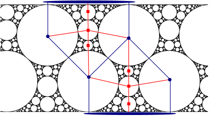
Figure 1: (Color online) Section of the $m,n=0$ bearing and the first generation of its contact network.

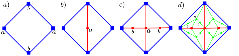
Figure 2: Hierarchical rule to construct the contact network for $m=n=0$. a) One starts with a loop of four nodes (two $a$- and two $b$-nodes) in a loop arrangement. b) A new $a$-node is added to the center of the loop and connected to the $b$-nodes on the top and bottom of the loop, dividing it into two loops. c) Two new $b$-nodes are also added, one inside of each loop and connected to the two closest $a$-nodes. The initial loop is now divided into four equal loops. d) The new generation is constructed in the same way inside each loop.

II.2 Degree distribution

We now provide an analytic expression for the degree distribution $P(k)$, where $k$ is the node degree (number of touching disks). Let us start with the number of nodes $N(g)$ at generation $g$, and neglect the first four nodes. One starts with one loop of two $a$- and two $b$-nodes at generation zero. At each generation, each loop is divided into four. Thus, the final number of loops is $4^{g}$. For each loop in generation $g-1$, one $a$- and two $b$-nodes are added to obtain the generation $g$, so that the number of $a$-nodes $N_{a}$ changes from generation $g-1$ to $g$ as,

$$\Delta N_{a}(g)=4^{g-1}$$ (1)

and the number of $b$-nodes $N_{b}$ as,

$$\Delta N_{b}(g)=2\cdot 4^{g-1}\ \ .$$ (2)

The number of nodes at generation $g$ is then,

$$N_{a}(g)=\sum_{t=1}^{g}4^{t-1}=\frac{4^{g}-1}{3}$$ (3)

and

$$N_{b}(g)=\sum_{t=1}^{g}2\cdot 4^{t-1}=\frac{2(4^{g}-1)}{3}\ \ ,$$ (4)

respectively. The total number of nodes $N$ is

$$N(g)=N_{a}(g)+N_{b}(g)=4^{g}-1\ \ .$$ (5)

At each generation, all $a$- and $b$-nodes receive one new link for each adjacent loop. Since the number of such loops equals the degree, the latter doubles at each generation. The new $a$-nodes have degree four, while the $b$-nodes have degree two. Hence, at generation $g$, the degree $k(t)$ of a node, added at generation $g_{0}$ that is part of the network for $t=g-g_{0}$ generations is,

$$k_{a}(g-g_{0})=4\cdot 2^{g-g_{0}}\ \ ,$$ (6)

$$k_{b}(g-g_{0})=2\cdot 2^{g-g_{0}}\ \ .$$ (7)

At generation $g$ the degree of a node is related to the generation $g_{0}$ at which the node was added. This generation is given by,

$$g-g_{0a}(k)=\frac{\ln(k/2)}{\ln 2}-1\ \ ,$$ (8)

and

$$g-g_{0b}(k)=\frac{\ln(k/2)}{\ln 2}\ \ .$$ (9)

The number of nodes of degree $k$ at generation $g$ equals the number of nodes added at generation $g_{0}(k)$, given by Eqs. (1) and (2). Thus, the degree distribution $P_{a}(k,g)$ is,

$$P_{a}(k,g) = \frac{\Delta N_{a}(g_{0a}(k))}{N_{a}(g)}$$ (10)

$$= 3\frac{4^{g}}{4^{g}-1}\left(\frac{k}{2}\right)^{-2}.$$

In the same way, $P_{b}(k,g)$ is,

$$P_{b}(k,g) = \frac{\Delta N_{b}(g_{0b}(k))}{N_{b}(g)}$$ (11)

$$= \frac{3}{4}\frac{4^{g}}{4^{g}-1}\left(\frac{k}{2}\right)^{-2}.$$

The total degree distribution $P(k,g)$ is then,

$$P(k,g) = \frac{\Delta N_{a}(g_{0a}(k))+\Delta N_{b}(g_{0b}(k))}{N(g)}$$ (12)

$$= \frac{3}{2}\frac{4^{g}}{4^{g}-1}\left(\frac{k}{2}\right)^{-2}.$$

In the limit $g\rightarrow\infty$,

$$P_{a}(k) = 3\left(\frac{k}{2}\right)^{-2}\ \ ,$$ (13)

$$P_{b}(k) = \frac{3}{4}\left(\frac{k}{2}\right)^{-2}\ \ ,$$ (14)

$$P(k) = \frac{3}{2}\left(\frac{k}{2}\right)^{-2}\ \ .$$ (15)

Thus, the degree distribution scales as $P(k)\propto k^{-\gamma}$, with $\gamma=2$, corresponding to a scale-free network. This exponent is larger than the one obtained for the Apollonian network, where $\gamma=\frac{\ln 3}{\ln 2}\approx 1.585$ Andrade Jr. et al. (2005). Note that the $a$/$b$ asymmetry disappears when one considers the two topological identical loops in the entire unit cell, for the $a$-nodes in the top loop correspond to the $b$-nodes in the bottom one.

II.3 Shortest paths and clustering coefficient

Spatial, self-similar networks are expected to exhibit some form of small-world behavior due to the confinement of connections Doye and Massen (2005), which is, for example, the case of the Apollonian network Zhang et al. (2008). Numerically, this can be checked by analyzing the size dependence of the average shortest path $l$, defined as the average minimum number of links necessary to form a connecting path between pairs of nodes in the network. Figure 3 shows that $l=a\ln N+b$, where $a$ and $b$ are constants, corresponding to a logarithmic scaling, as expected for small-world networks Watts and Strogatz (1998).

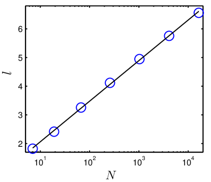
Figure 3: Size dependence of the average shortest path $l$, for the contact network of bearings of $m=n=0$, where $N$ is the number of nodes. The shortest path scales logarithmically with the number of nodes, $l=0.61\ln{N}+0.65$ as expected for small-world networks.

Small-world networks are typically highly clustered Watts and Strogatz (1998). To quantify the degree of clustering one measures the clustering coefficient $C$, defined for each node as the fraction of pairs of neighbors that are directly connected, forming a triangle. In the case of bearings, all loops have a even number of nodes, the contact network is bipartite, and two neighbors of a node are never directly connected. Lind et al. Lind et al. (2005) proposed a new clustering coefficient for bipartite networks $C_{4}$, defined as the fraction of pairs that are indirectly connected through one single node, forming a loop. Then, for a node of degree $k$,

$$C_{4}=\frac{\#(\text{Indir. conn. between neighb.})}{k(k-1)/2}.$$ (16)

In the following we will use this definition. First, we calculate $C_{4a/b}(t)$, the clustering coefficient of an $a$/$b$-node that was added to the network $t$ generations before. At each iteration, the degree of every node is doubled, by adding new neighbors. Each new neighbor is connected via a new node to other two neighbors (see Fig. 2). Thus, the number of indirectly connected pairs of neighbors increases at each generation by twice the node degree. Every new $a$-node has degree four and from its six different pairs of neighbors, five are indirectly connected. Every new $b$-node has degree two and its pair of neighbors is always indirectly connected. By summing over generations, one gets for $a$-nodes,

$$C_{4a}(t) = \frac{5+\sum_{i=0}^{t-1}2\cdot k_{a}(i)}{k_{a}(t)(k_{a}(t)-1)/2}$$ (17)

$$= \frac{3}{2}2^{-t}-\frac{2}{4\cdot 2^{t}-1},$$

and for $b$-nodes,

$$C_{4b}(t) = \frac{1+\sum_{i=0}^{t-1}2\cdot k_{b}(i)}{k_{b}(t)(k_{b}(t)-1)/2}$$ (18)

$$= 3\cdot 2^{-t}-\frac{2}{2\cdot 2^{t}-1},$$

where we employed Eqs. (6) and (7). Once again, note that the $a$/$b$ asymmetry is only observed when we solely consider one loop. For the entire stripe, the top and bottom loops of the unit cell are equivalent, but the $a$-nodes of the top loop are $b$-nodes of the bottom one. Thus, when the entire unit cell is considered, the network is completely symmetric with respect to $a$ and $b$. Both coefficients tend to zero as $C_{4}(t)\sim 2^{-t}$ for $t\rightarrow\infty$. The clustering of the entire network can be evaluated from the average over all nodes,

$$C_{4}(g)=\sum_{t=1}^{g}\frac{\Delta N_{a}(t)C_{4a}(g-t)+\Delta N_{b}(t)C_{4b}(g-t)}{N(g)}.$$ (19)

We evaluate this sum numerically as shown in Fig. 4, for different number of nodes in the network, and obtain that $C_{4}\approx 0.8625$ in the thermodynamic limit.

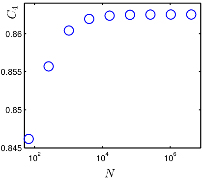
Figure 4: Clustering coefficient $C_{4}$ for the contact network of bearings of $m=n=0$ as a function of the number of nodes $N$.

II.4 Bond percolation

We now study bond percolation on a network corresponding to a unit-cell of the stripe, consisting of two initial squares sharing one link (see Fig. 1). We focus on the existence of a spanning cluster between the two nodes representing the top and bottom surfaces, respectively. To compute the percolation threshold, we performed Monte Carlo simulations for different values of bond occupation probability $p$ and network size $N$. We estimate the threshold $p_{c}$ as the value of $p$ at which the probability of spanning is $1/2$. We employed the bisection method and considered values of $p$ that differ by $0.001$. Figure 5 shows the size dependence of the estimated value of $p_{c}$, where one clearly sees that $p_{c}$ vanishes in the thermodynamic limit. Asymptotically, the decay follows a power-law $p_{c}\sim N^{-\frac{1}{2\nu}}$, with $\nu\approx 7$. The same threshold is observed for the Apollonian network and other scale-free networks with $\gamma<3$. However, the convergence to the thermodynamic value is much slower here than for the Apollonian network, where $\nu\approx 3$ Andrade Jr. et al. (2005).

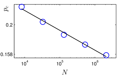
Figure 5: Dependence o the percolation threshold $p_{c}$ on the network size $N$. The black line corresponds to the least-squares fit to the data of a power-law, $p_{c}\sim N^{-frac{1}{2\nu}}$, with exponent $\nu=7\pm 1$.

III General case

III.1 The network construction

$m=0,n=0$	$m=0,n=1$	$m=0,n=2$
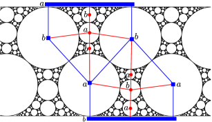
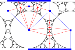
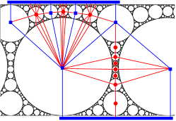
$m=1,n=0$	$m=1,n=1$	$m=1,n=2$
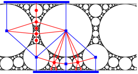
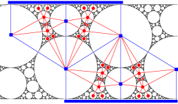
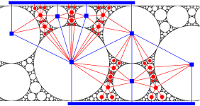
$m=3,n=0$	$m=3,n=1$	$m=3,n=2$

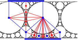
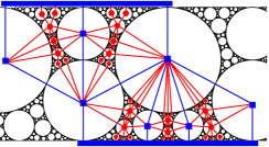
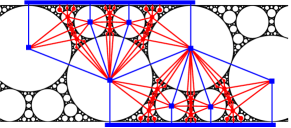
Figure 6: (Color online) Examples of space-filling bearings of the first family, for different values of $m$ and $n$.

We now consider the general case of the contact network for a bearing in the first family for loops of size four with any $m$ and $n$. Figure 6 shows examples of bearings generated with different $m$ and $n$, with the respective contact network on top. For all cases, the unit cell consists of loops of size four with the largest disks, including the top and bottom surfaces, respectively. However, the number of such loops varies with $m$ and $n$ and the rotation symmetry is broken for $m\not=n$. At each iteration the number of vertical and horizontal new loops constructed inside each loop also depends on $m$ and $n$, respectively. As summarized in Fig. 7, we first discuss how to determine the initial number of loops in the unit cell (left panel) and proceed discussing how to hierarchically fill each loop (right panel).

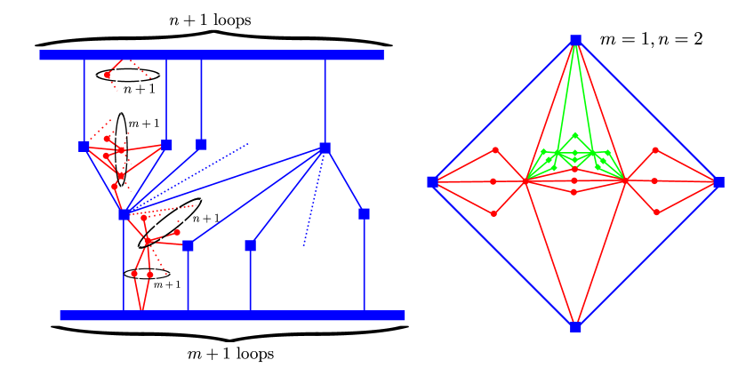
Figure 7: (Color online) The left panel shows a sketch of the initial network set up (blue, sites drawn as squares) and the first generation in the general case (red, sites as dots). In the right panel are the first two generations and part of the second (green) for $m=1$ and $n=2$.

For all values of $m$ and $n$, the unit cell of the bearing consists of a top and a bottom part. The number of initial loops on top and bottom equals $n+1$ and $m+1$, respectively (see loops of blue-square nodes in Fig. 6 and left panel in Fig. 7). Note that the $(m,n)$ configuration is equivalent to the $(n,m)$ configuration after a rotation of $\pi$ around the point where the common edge of the top and bottom loops crosses the middle of the stripe. To hierarchically construct the network one starts with the $n+1$ top and $m+1$ bottom loops. Hereafter, we solely consider one top and a bottom loop (sharing one edge), as the construction of the other loops is straightforward. To form the first generation we first add $m+1$ $a$-nodes to the top loop and connect them to the two existing (lateral) $b$-nodes, dividing the initial loop into $m+2$ loops. Then, in each new loop, we add $n+1$ $b$-nodes and connect them to the top and bottom $a$-nodes. We are left with $(n+2)(m+2)$ loops inside the top loop. Second, we construct the interior of the bottom loop. There, we start by adding $n+1$ $b$-nodes and connect them to the two existing (lateral) $a$-nodes. Then, in each one of the new $n+2$ loops we add $m+1$ $a$-nodes and connect them to the top and bottom $b$-nodes. In the bottom, we are also left with $(n+2)(m+2)$ loops. Proceeding iteratively in the same way, we hierarchically construct the entire contact network of the space-filling bearing, for any $m$ and $n$.

III.2 Degree distribution

We now provide an analytic expression for the degree distribution $P_{m,n}(k)$ for any $m$ and $n$, following the same strategy as for $m=n=0$ in Sec. II.2. For simplicity, we restrict the calculation to networks inside a single loop (one initial top loop), as the total degree distribution of the unit cell is straightforwardly obtained as a weighted average of $P_{m,n}(k)$ and $P_{n,m}(k)$, corresponding to the degree distribution in the top and bottom loops, where the statistical weights are given by the initial fraction of top $(n+1)$ and bottom $(m+1)$ loops, respectively.

At each generation, $(n+2)(m+2)$ loops are constructed for every loop in the previous generation. As before, we neglect the initial set of nodes. At generation $g-1$ there are $(n+2)^{g-1}(m+2)^{g-1}$ loops. Thus, from generation $g-1$ to $g$, the change in the number of $a$-nodes is,

$$\Delta N_{a}(g)=(m+1)\left[(n+2)(m+2)\right]^{g-1}\ \ ,$$ (20)

and in the number of $b$-nodes is,

$$\Delta N_{b}(g)=(m+2)(n+1)\left[(n+2)(m+2)\right]^{g-1}\ \ ,$$ (21)

corresponding to $(m+1)$ new $a$- and $(m+2)(n+1)$ new $b$-nodes per loop. The number of nodes at generation $g$ is then,

$$N_{a}(g) = (m+1)\sum_{t=1}^{g}\left[(n+2)(m+2)\right]^{t-1}$$ (22)

$$= \frac{(m+1)\left(\left[(n+2)(m+2)\right]^{g}-1\right)}{(n+2)(m+2)-1},$$

and

$$N_{b}(g) = (m+2)(n+1)\sum_{t=1}^{g}\left[(n+2)(m+2)\right]^{t-1}$$ (23)

$$= \frac{(m+2)(n+1)(\left[(n+2)(m+2)\right]^{g}-1)}{(n+2)(m+2)-1},$$

respectively. The total number of nodes $N$ is,

$$N(g)=N_{a}(g)+N_{b}(g)=\left[(n+2)(m+2)\right]^{g}-1.$$ (24)

The degree $k$ of a node increases monotonically with the generation. An $a$-node has initially degree $2(n+2)$ and its degree increases by a factor of $n+2$ at each generation. Thus, at generation $g$, the degree of an $a$-node added at generation $g_{0}$ is,

$$k_{a}(g-g_{0})=2(n+2)^{g-g_{0}+1}\ \ .$$ (25)

A $b$-node has initially degree two and its degree increases by a factor of $m+2$ at each generation. Thus, at generation $g$, the degree of a $b$-node added at generation $g_{0}$ is,

$$k_{b}(g-g_{0})=2(m+2)^{g-g_{0}}\ \ .$$ (26)

Consequently, the node of degree $k$ at generation $g$ that was added at generation $g_{0}$ is given by,

$$g-g_{0a}(k)=\frac{\ln(k/2)}{\ln(n+2)}-1\ \ ,$$ (27)

for $a$-nodes and

$$g-g_{0b}(k)=\frac{\ln(k/2)}{\ln(m+2)}\ \ ,$$ (28)

for $b$-nodes. The degree distribution for the $a$-nodes in the loop is then,

$$P^{a}_{m,n}(k,g) = \frac{\Delta N_{a}(g_{0a}(k))}{N_{a}(g)}$$ (29)

$$= \left[(n+2)(m+2)-1\right]f_{m,n}(g)\left(\frac{k}{2}\right)^{-\left[1+\frac{\ln(m+2)}{\ln(n+2)}\right]},$$

where,

$$f_{m,n}(g)=\frac{\left[(n+2)(m+2)\right]^{g}}{\left[(n+2)(m+2)\right]^{g}-1}\ \ .$$ (30)

For the $b$-nodes is,

$$P^{b}_{m,n}(k,g) = \frac{\Delta N_{b}(g_{0b}(k))}{N_{b}(g)}$$ (31)

$$= \frac{(n+2)(m+2)-1}{(n+2)(m+2)}f_{m,n}(g)\left(\frac{k}{2}\right)^{-\left[1+\frac{\ln(n+2)}{\ln(m+2)}\right]}.$$

And the total degree distribution $P_{m,n}(k,g)$ is,

$$P_{m,n}(k,g) = \frac{\Delta N_{a}(g_{0a}(k))+\Delta N_{b}(g_{0b}(k))}{N(g)}$$ (32)

$$= f_{m,n}(g)\left[(m+1)\left(\frac{k}{2}\right)^{-\left[1+\frac{\ln(m+2)}{\ln(n+2)}\right]}\right.$$

$$\left.+\frac{n+1}{n+2}\left(\frac{k}{2}\right)^{-\left[1+\frac{\ln(n+2)}{\ln(m+2)}\right]}\right].$$

In the limit $g\rightarrow\infty$,

$$P_{m,n}(k) = (m+1)\left(\frac{k}{2}\right)^{-\left[1+\frac{\ln(m+2)}{\ln(n+2)}\right]}$$ (33)

$$+\frac{n+1}{n+2}\left(\frac{k}{2}\right)^{-\left[1+\frac{\ln(n+2)}{\ln(m+2)}\right]}\ \ .$$

When $m=n$, $\gamma=2$ is recovered Doye and Massen (2005). For $m\not=n$, the degree distribution is a sum of two power laws. Asymptotically, for $k\rightarrow\infty$, $P_{m,n}(k)$ is dominated by the term with the smallest exponent and thus

$$\gamma=\min\left\{1+\frac{\ln(m+2)}{\ln(n+2)},1+\frac{\ln(n+2)}{\ln(m+2)}\right\}\ \ .$$ (34)

The contact network of a bearing is always a scale-free network of $1<\gamma\leq 2$, as shown in Fig. 8.

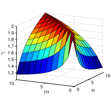
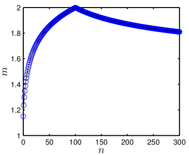
Figure 8: (Color online) Left: Degree exponent $\gamma$ as a function of $m$ and $n$. Note that, $\gamma=2$ for $m=n$. Right: Degree exponent $\gamma$ as a function of $n$ for $m=100$.

Note that the degree exponent is symmetric to permutations of $m$ and $n$. The degree distribution of the entire unit cell is symmetric at every generation as it is given by,

$$P(k) = \frac{(n+1)P_{m,n}(k)+(m+1)P_{n,m}(k)}{m+n+2}$$ (35)

$$= \frac{\left[(n+1)(m+1)+\frac{(m+1)^{2}}{m+2}\right]\left(\frac{k}{2}\right)^{-\left[1+\frac{\ln(m+2)}{\ln(n+2)}\right]}}{m+n+2}$$

$$+ \frac{\left[\frac{(n+1)^{2}}{n+2}+(n+1)(m+1)\right]\left(\frac{k}{2}\right)^{-\left[1+\frac{\ln(n+2)}{\ln(m+2)}\right]}}{m+n+2}\ \ .$$

III.3 Shortest path and clustering coefficient

We numerically analyze the size dependence of the average shortest path $l$ for all combinations of $n,m=0,1,2,3,4$. For all cases, we find a logarithmic scaling of $l$ with the number of nodes, consistent with small-world networks. For $m=n$ we find that the prefactor of the logarithmic scaling is independent on the value of the indices, as also observed for $\gamma$. If $m\not=n$, then the prefactor changes with $m$ and $n$ as shown in Fig. 9, for example, for fixed $m=0$, the prefactor decreases with $n$.

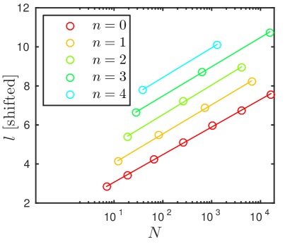
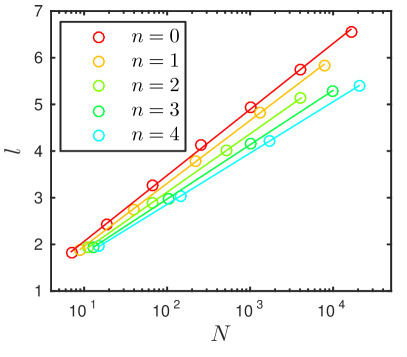
Figure 9: Left: Average shortest path $l$ as a function of the number of nodes $N$ for $n=m$. Lines were shifted vertically by adding $n$ for better visualization. Right: Average shortest path $l$ as a function of the number of sites $N$ for $m=0$. Lines were also shifted vertically. The lines are just guides to the eye.

Next, we calculate $C_{4}$. A new $a$-node has (n+3)(n+2)-1 pairs of neighboring $b$-nodes connected indirectly through one $a$-node. At each generation, when new neighbors are added to each loop adjacent to this $a$-node, the number of connected pairs increases by (n+3)(n+2)/2-1. Hence, an $a$-node that was added to the network at generation $g_{0}$, and is part of the network for $t=g-g_{0}$ generations, has clustering coefficient,

$$C_{4a}(t) = \frac{(n+3)(n+2)-1+\left[\frac{(n+3)(n+2)-1}{2}-1\right]\sum_{i=0}^{t-1}k_{a}(i)}{k_{a}(t)(k_{a}(t)-1)/2}$$

$$= \frac{(n+3)(n+2)-1}{(n+2)^{t+1}\left[2(n+2)^{t+1}-1\right]}+\frac{2(n+2)\left[\frac{(n+3)(n+2)-1}{2}-1\right]\frac{(n+2)^{t}-1}{n+1}}{(n+2)^{t+1}\left[2(n+2)^{t+1}-1\right]}$$

$$\sim (n+2)^{-t}\text{ as }t\rightarrow\infty\ \ .$$

Initially, for $b$-nodes there is only one pair of neighbors indirectly connected and $\frac{(m+3)(m+2)}{2}-1$ connections are added per adjacent loop at each iteration. Thus,

$$C_{4b}(t) = \frac{1+\left[\frac{(m+3)(m+2)-1}{2}-1\right]\sum_{i=0}^{t-1}k_{b}(i)}{k_{b}(t)(k_{b}(t)-1)/2}$$

$$= \frac{1+2\left[\frac{(m+3)(m+2)-1}{2}-1\right]\frac{(m+2)^{t}-1}{m+1}}{(m+2)^{t}(2(m+2)^{t}-1)}$$

$$\sim (m+2)^{-t}\text{ as }t\rightarrow\infty.$$

The argument of the power law is different for $a$- and $b$-nodes as it depends on $n$ and $m$, respectively. Both $C_{4a}$ and $C_{4b}$ asymptotically vanish. The faster the degree of a node type grows the faster its $C_{4}$ falls off.

III.4 Bond percolation

We performed simulations of the bond percolation model on a unit-cell for different pairs of indices $m,n$. As in Sec. II.4, we define the spanning cluster as a set of connected nodes that include the top and bottom surfaces. Note that the top and bottom surfaces correspond to different types of nodes, $a$ and $b$, respectively (see Fig. 6).

For all considered values of $m$ and $n$ we find that the percolation threshold $p_{c}$ vanishes in the thermodynamic limit (infinite system size) and the estimator for the threshold scales as $p_{c}(N)\sim N^{-\frac{1}{2\nu}}$. Our results for $m=n$ suggest that $\nu$ does not change with the bearing indices ($m$ and $n$), like we also found for the degree exponent $\gamma$ in Sec. III.2. Since the number of nodes in the network grows exponentially with the generation, we refrain from performing a detailed size-dependence analysis to obtain $\nu$ with high precision.

IV Final remarks

We studied the contact network of space-filling bearings of loops of size four in the first family. We proposed a hierarchical rule to construct the network and provided analytic expressions for the degree distribution and clustering coefficient. We also studied numerically the shortest path and percolation properties. We showed that the exponent $\gamma$ changes in the range $(1,2]$ and that is always two when $m=n$. Numerical simulations also suggest that the correlation exponent $\nu$ for the percolation transition does not change with the bearing indices. Our networks are bipartite and we find that if $m\not=n$ the degree distribution of the two species scale with different exponents inside each loop. To our knowledge, this is the first example of an artificial hierarchical network exhibiting this property which has already been observed empirically for sexual networks Blasio et al. (2007).

We are proposing a method to generate deterministic hierarchical scale-free networks of different $\gamma$ exponents, which are amenable to analytic treatment. As it was accomplished for the Apollonian network, possible extensions of our work include the study of their magnetic, spectral, and dynamical properties Moreira et al. (2006); de Oliveira et al. (2009, 2010). Other possibilities include the study of the networks of random space-filling or three-dimensional bearings, larger loops and second family of bearings.